

Abstract
Objective. Persons with tetraplegia can use brain-machine interfaces to make visually guided reaches with robotic arms. Without somatosensory feedback, these movements will likely be slow and imprecise, like those of persons who retain movement but have lost proprioception. Intracortical microstimulation (ICMS) has promise for providing artificial somatosensory feedback. ICMS that mimics naturally occurring neural activity, may allow afferent interfaces that are more informative and easier to learn than stimulation evoking unnaturalistic activity. To develop such biomimetic stimulation patterns, it is important to characterize the responses of neurons to ICMS. Approach. Using a Utah multi-electrode array, we recorded activity evoked by both single pulses and trains of ICMS at a wide range of amplitudes and frequencies in two rhesus macaques. As the electrical artifact caused by ICMS typically prevents recording for many milliseconds, we deployed a custom rapid-recovery amplifier with nonlinear gain to limit signal saturation on the stimulated electrode. Across all electrodes after stimulation, we removed the remaining slow return to baseline with acausal high-pass filtering of time-reversed recordings. Main results. After single pulses of stimulation, we recorded what was likely transsynaptically-evoked activity even on the stimulated electrode as early as ∼0.7 ms. This was immediately followed by suppressed neural activity lasting 10–150 ms. After trains, this long-lasting inhibition was replaced by increased firing rates for ∼100 ms. During long trains, the evoked response on the stimulated electrode decayed rapidly while the response was maintained on non-stimulated channels. Significance. The detailed description of the spatial and temporal response to ICMS can be used to better interpret results from experiments that probe circuit connectivity or function of cortical areas. These results can also contribute to the design of stimulation patterns to improve afferent interfaces for artificial sensory feedback.
Export citation and abstract BibTeX RIS

Original content from this work may be used under the terms of the Creative Commons Attribution 4.0 license. Any further distribution of this work must maintain attribution to the author(s) and the title of the work, journal citation and DOI.
1. Introduction
Efferent brain-machine interfaces (BMIs) have advanced to the point where a spinal-cord injured patient can move a robotic arm using signals recorded from motor cortex (Hochberg et al 2012, Collinger et al 2013, Wodlinger et al 2014). Without somatosensory feedback, the effectiveness of the movements generated through these interfaces will be limited, perhaps like those of people who have lost somatosensation (Ghez et al 1990, Sainburg et al 1995). Intracortical microstimulation (ICMS), which has been shown to elicit percepts in rats, monkeys, and humans (Romo et al 2000, London et al 2008, Fridman et al 2010, Devecioğlu and Güçlü 2017), is a promising approach for providing artificial somatosensory feedback via an afferent interface (Tabot et al 2013, Flesher et al 2016). In the first such bidirectional BMI, monkeys could move a virtual arm to explore the 'texture' of different virtual objects, a property conveyed by two different temporal patterns of ICMS (O'Doherty et al 2011). The monkeys moved the arm sequentially to the objects to find the one with the rewarded texture. More advanced methods have been used to supply a spinal-cord injured patient with information about object contact location and force (Flesher et al 2016, 2021). Using a robotic arm, the patient was able to pick up, move, and place objects faster using vision combined with ICMS feedback than with visual feedback alone, primarily because they spent less time attempting to grasp the object (Flesher et al 2021).
While some proprioceptive sensations have been elicited with ICMS (Salas et al 2018), achieving usable feedback about the position and movement of the arm has proven more difficult than providing the analogous artificial sense of touch. In one approach, monkeys learned to reach to invisible targets using ICMS feedback through eight arbitrarily chosen electrodes which provided information about the error vector between hand and target position (Dadarlat et al 2015). Monkeys only learned to use this feedback after a few months of training. To shorten this long learning period, it may be possible for ICMS to provide more naturalistic feedback (Bensmaia and Miller 2014). In a second approach, researchers attempted to evoke perceptions of hand movement by stimulating on small sets of electrodes in somatosensory cortical area 2 that had similar preferred directions (Tomlinson and Miller 2016). This biomimetic approach was successful for six of seven sets of electrodes in one monkey but failed in three other monkeys. The difference across monkeys may have been due to differences in array placement or the particular population of neurons activated by stimulation. Had it been possible to monitor the homogeneity of preferred directions of activated neurons, the explanation may have been clearer.
To better interpret experiments which use ICMS and to achieve more successful mimicry of naturally occurring activity, it will likely be important to quantify the evoked response of neurons to a range of stimulus parameters. However, recording at short latency after stimulation is difficult due to the large shock artifact it causes (Hao et al 2016, Weiss et al 2018). Many experiments have been limited to recordings made on distant electrodes, hundreds of microns away or even on a separate array (Butovas and Schwarz 2003, Hao et al 2016, Chen et al 2020, Allison-Walker et al 2021), thereby missing evoked activity near the stimulated electrode. Further, previous studies have typically characterized the evoked response to only single pulses of stimulation, whereas future afferent interfaces will need to employ trains of stimulation throughout a grasp and/or movement (Flesher et al 2021).
We developed novel hardware and software techniques allowing us to record ∼0.7 ms after stimulation offset on every electrode in an implanted microelectrode array, including even the stimulated one. With these methods we first used single pulses across a wide range of amplitudes to characterize the short-latency excitatory and long-lasting inhibitory responses of neurons recorded on the stimulated electrode, as was done previously for non-stimulated electrodes (Butovas and Schwarz 2003, Hao et al 2016). In preliminary experiments, we noticed that the evoked response on the stimulated electrode decreased rapidly throughout ∼0.2 s, high-frequency trains, and that neurons greatly increased their firing rates for ∼0.1 s after the end of the train. We extended the train length to 4 s, more akin to the prolonged stimulation provided by an afferent interface (Flesher et al 2021). During these longer trains, the excitatory response recorded on the stimulated electrode decayed, while the response on non-stimulated electrodes was typically maintained throughout the train. The results in this paper can inform the interpretation and design of stimulation patterns for providing somatosensory feedback.
2. Methods
2.1. Animal subjects
We performed experiments using two male rhesus macaques. Monkey H was 12.0 kg and monkey D was 10.0 kg when we performed the experiments. We performed all procedures in this study in accordance with the Guide for the Care and Use of Laboratory Animals. The institutional animal care and use committee of Northwestern University approved all procedures in this study under protocol #IS00000367.
2.2. Implant and data collection
Each monkey was implanted with a 96-electrode sputtered iridium-oxide multi-electrode array with 1.0 mm electrodes (Blackrock Neurotech, Salt Lake City, UT) in the proximal arm area of somatosensory cortical area 2. In addition to surface landmarks, we recorded intraoperatively from the cortical surface while manipulating the arm and hand to find the arm representation (for more details, see Weber et al 2011). We performed sensory mappings after implantation to confirm that recorded neurons had receptive fields corresponding to the proximal arm.
We used the Blackrock Stim Headstage, Front-End amplifier, and Neural Signal Processor (Blackrock Neurotech, Salt Lake City, UT) to record signals at 30 kHz. We delivered ICMS from the Blackrock CereStim R96. Unless otherwise noted, electrodes were stimulated with biphasic pulses, each phase lasting 200 μs and separated by 53 μs. We used the sync line from the CereStim R96 to determine stimulation onset, accounting for the 60 μs delay between sync line going high and stimulation.
During all experiments, monkeys performed a center-out reaching task while holding the handle of a robotic manipulandum (for more details, see (London and Miller 2012)) or sat idly in the chair. Stimulation was delivered independently of the monkey's behavior.
2.3. Pipeline to record at short latencies after ICMS
Typically, ICMS causes large electrical artifacts which prevent neural recordings for an extended period after stimulation. When using the Blackrock Stim Headstage and Front-End amplifier to record on the stimulated electrode, the recorded signal saturated the amplifier for several milliseconds (figure 1(a), dashed lines), after which the signal slowly recovered to baseline. To enable recording at shorter latencies, we developed a rapid-recovery amplifier (RRA, see supplementary materials available online at stacks.iop.org/JNE/19/026044/mmedia) and used it instead of the Blackrock Stim Headstage and Front-end Amplifier. We used a custom-made breakout board to pass a single channel from the Cereport to the RRA, bypassing the Stim Headstage (see supplementary materials). The RRA has several features that allow it to operate on the same electrode as the stimulator, yet still recover rapidly after stimulation. The wide input range (±15 V) of the first stage of the RRA prevents the need for input voltage clamping and current shunting as well as output saturation during the stimulus pulse. To prevent saturation of subsequent stages, the gain of the RRA declines rapidly from a maximum of ∼1000 to a minimum of one during large dynamic swings of the front-end voltage. The output of the RRA, which was limited to ±5 V, was connected to an analog input on the Blackrock Neural Signal Processor (figure 1(b)).
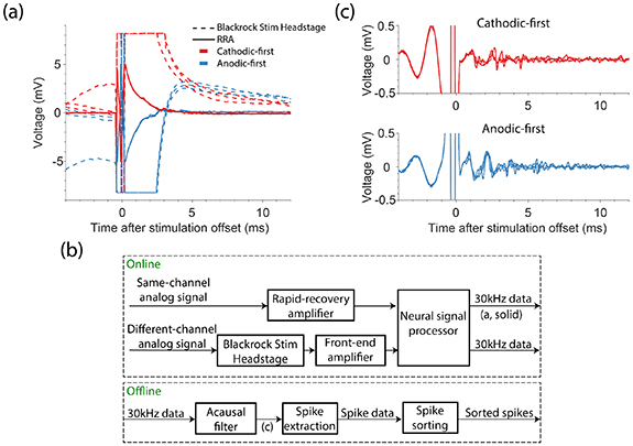
Figure 1. Overview of artifact reduction pipeline. (a) Example recordings from the stimulated channel are shown when recording with the Blackrock Stim Headstage and Front-end amplifier (dashed lines) and our rapid recovery amplifier (RRA; solid lines). We stimulated with anodic-first (blue) or cathodic-first (red) biphasic pulses with phase duration of 200 μs, phases separated by 53 μs, and with an amplitude of 50 µA. (b) Block diagram depicting the artifact reduction pipeline. The rapid-recovery amplifier receives signals and passes them to the Blackrock Neural Signal Processor. Signals from channels that were not stimulated were amplified by the Blackrock Stim Headstage and Front-End amplifier. All signals were sampled at 30 kHz and filtered offline. After filtering, we extracted spikes via threshold crossings and then sorted the spike data. (c) Voltages recorded using the RRA after acausal time-reversed high-pass filtering. Traces in (c) correspond to those in (a).
Download figure:
Standard image High-resolution imageTo measure the progressive gain recovery of the RRA after stimulation when stimulating and recording on the same electrode, we monitored the size of the artifact evoked by much lower current stimulation on a remote electrode. We tested gain recovery following alternating cathodic- and anodic-first biphasic pulses at 10 Hz, with amplitudes of 5–30 μA in 5 μA steps and 40–100 μA in 10 μA steps. We tested 25 stimulation electrodes across the two monkeys and delivered 32 ± 2 (mean ± sd) pulses per condition. The remote channel was stimulated at 3000 Hz for 4.5 ms, with cathodic-first biphasic pulses (53 μs pulse length with 53 μs between phases). We used 1 μA to monitor gain recovery on four stimulation electrodes in one session, and 5 μA on the remote channel in later sessions.
Even with the RRA, full recovery to baseline took ∼3 ms (figure 1(a), solid lines). While a high-pass filter removed this drift, ringing caused by filtering the large artifact prevented neural recording for ∼10 ms. Instead, we applied a 500 Hz high-pass Butterworth filter acausally, backwards in time, thereby preventing the introduction of a ringing artifact (figure 1(c)). We adjusted the timestamps of recorded spikes to account for the ∼100 μs phase shift caused by filtering. Even with this acausal filtering we avoided filtering through the artifact, which would have obscured the pre-stimulus data (as seen in figure 1(c)). To account for the changing gain of the RRA, we divided the recorded signal by the measured gain recovery. After filtering, we extracted neural activity by finding threshold crossings and then sorting single units using OfflineSorter (Plexon Inc., Dallas, TX).
Recordings on non-stimulated electrodes using the Stim Headstage and Front-end Amplifier were saturated for ∼0.7 ms after stimulation offset. In our testing, the RRA did not shorten the recording latency on non-stimulated electrodes. Because of this, we did not use the RRA when recording on non-stimulated channels. Nevertheless, we filtered acausally before extracting neural activity as we did for recordings made on the stimulated electrode.
2.4. Evaluating the performance of the RRA and acausal, time-reversed filtering
To evaluate the performance of our pipeline for recording neural activity on the stimulated electrode, we tested how well we could recover simulated activity, added artificially at different latencies after stimulation. For this simulation, we recorded in the presence of artifacts with either the RRA or the Stim Headstage and Front-End amplifier on ten representative stimulation electrodes. To simulate neural activity, we recorded naturally occurring spike waveforms during a period without stimulation, which we added to the recordings at random times after stimulation. We added spike waveforms at random latencies between 0.2–7 ms following 50% of the stimuli for each of the ten electrodes. For each electrode, we generated 200 000 stimulation artifacts, half from recordings made with the RRA and half with the standard Blackrock hardware. We tested the same amplitudes described above for measuring RRA gain but used only cathodic-first pulses since our subsequent experiments used this polarity. We computed the percentage of spikes recovered by comparing the time stamps of recovered spikes to the artificial ones, tolerating ±0.33 ms of error.
2.5. Stimulation protocol for characterizing the evoked response
After evaluating our recording capability, we characterized the response evoked on the stimulated channel by single pulses or pulse trains. Table 1 shows the numbers of sessions for each monkey, electrodes tested, neurons recorded, and trains per condition for all experiments. The final column (inter-train period) indicates the time between successive stimulation conditions. We slightly jittered the inter-train period for each condition to prevent synchronizing stimulation with any physiological process by adding 0–100 ms sampled from a uniform distribution. We measured the progressive gain recovery of the RRA at each stimulation amplitude for each stimulation electrode.
Table 1. Experimental parameters are shown for the single pulse, short train, and the continuous (Cont.) long train experiments when recording on either the stimulated channel (stim) or non-stimulated channels (nonstim). The numbers of sessions for monkey H and monkey D are denoted with 'H' and 'D' respectively.
| # sessions | # stimulation electrodes | # neurons | # pulses or trains (mean ± std.) | Inter-train period (s) | |
|---|---|---|---|---|---|
| Single Pulse | 4 H; 4 D | 29 | 30 | 82.6 ± 14.4 | 0.5 |
| Short Train | 7 H; 5 D | 19 | 19 | 253 ± 17.2 | 0.5 |
| Cont. Long Train (stim) | 6 H; 4 D | 24 | 25 | 8 ± 0 | 20 |
| Cont. Long Train (nonstim) | 6 H; 4 D | 24 | 437 | 8 ± 0 | 20 |
In initial experiments we measured the response evoked by single pulses at a range of amplitudes typically used in BMIs (Rajan et al 2015, Salas et al 2018, Flesher et al 2021). In four experiments, we tested 10–60 μA in 10 μA steps, 80 and 100 μA. Later, we probed the lower stimulation amplitudes more thoroughly using 10–30 μA in 5 μA steps and 40, 50, and 100 μA for another four electrodes, then added a 5 μA condition for the final 21 electrodes.
We next characterized the responses to short (∼0.2 s) trains. We stimulated at 50 μA and at 20, 49, or 94 Hz for seven channels, from which we recorded seven neurons. After noticing a modest decay in the neuronal responses throughout the 0.2 s train at 94 Hz, we added a 179 Hz conditionwhen we recorded the final 12 neurons. After short, high frequency trains, we observed rebound excitation, which we analyzed with this data.
We then characterized the evoked response to longer (∼4 s) trains of stimulation, a duration that approximates that required for a BMI user to grasp an object (Flesher et al 2021). Because the recorded neural response decayed rapidly with 179 Hz stimulation, we used a maximum of 131 Hz when stimulating with 4 s long trains. We stimulated with all combinations of 51, 80, 104, 131 Hz and 20, 40, 60 μA, amplitudes, these ranges chosen to evoke robust responses. While delivering continuously varying sensory feedback will require trains with time-varying amplitude or frequency, testing that full parameter space would not be feasible. Thus, we used trains with constant stimulation parameters to partially sample the space. Data were collected simultaneously on the stimulated and non-stimulated channels during this experiment. The results for non-stimulated channels may include a given neuron activated by different stimulation electrodes.
2.6. Data analysis
All data analysis was performed using MATLAB (MathWorks Inc., Natick, MA). To quantify the amount of activity evoked by each pulse, we counted spikes between 0.5 and 5.0 ms after the offset of each pulse and averaged across pulses. To account for different baseline firing rates across neurons, we subtracted the expected number of spontaneous spikes based on the baseline firing rate measured 10 –80 ms before onset of single pulses or 0.2–2 s before train onset.
We computed an activation threshold for each neuron in response to single pulses. To do so, we measured the proportion of stimulation pulses with at least one spike occurring 0.5–5 ms after stimulation offset for each condition and neuron. We defined the activation threshold as the smallest amplitude at which the proportion of trials with a spike was significantly larger than that expected based on the baseline firing rate (Chi-Square test, α < 0.05). We determined if a neuron was responsive to long trains of stimulation in a similar manner. Since the evoked response decayed throughout long trains, we considered only the first 20 pulses in each train. For each condition, neurons with significantly more spikes than chance (Chi-Square test, α < 0.05) were considered responsive.
Multiple spikes were typically evoked at consistent latencies by single stimulus pulses. We grouped spikes based on their response latency across trials for each neuron and condition. To do so, we computed a firing rate for the spikes by convolving them with a non-causal Gaussian kernel of width equal to a standard deviation of 0.2 ms, which we then averaged across pulses. We found peaks in this average with MATLAB's findpeaks algorithm. This algorithm uses 'prominence', the height of a peak and its location relative to other peaks, to measure how much a peak stands out (for more details, see supplementary materials for more details). We required peaks to have a minimum prominence of 1.0 and to be separated by at least 0.7 ms. This algorithm also computes the width at half maximum of each peak. Spikes that occurred within the width of each peak were included in the corresponding group. We measured the latency of each peak and computed the standard deviation of the spike times within each group. Our results were only slightly affected by small changes to the smoothing kernel width, minimum peak spacing, and minimum prominence.
After an evoked response, many neurons underwent either long-lasting inhibition or rebound excitation, which we quantified by computing the average firing rate across trials using a two-bin running average across 5 ms bins. We defined an inhibitory response as a firing rate below three-quarters of the mean baseline firing rate for two consecutive bins (a similar threshold as (Butovas and Schwarz 2003)) and measured the time the firing rate remained below this threshold. We defined a rebound excitatory response if two consecutive bins exceeded twice the mean baseline firing rate and the corresponding duration.
For many neurons, the evoked response decreased throughout long trains of stimulation. We measured the decay rate for each responsive neuron. To do so, we measured the mean firing rate in 50 ms bins from 0.0–3.9 s after train onset, excluding the initial 1 ms after each pulse, which was obscured by the stimulus artifact. We then fit the firing rate with an exponential decaying function,

with  as the intercept and
  as the decay rate. A large decay rate indicates the response decayed rapidly, while a decay rate near zero indicates the response was maintained throughout the train.
2.7. Statistical analysis
We used linear and logistic models to analyze many of our results statistically. We included two interaction terms in the model when analyzing the effect of amplitude, time, and amplifier on the proportion of simulated spikes recovered: one between amplitude and amplifier, to test whether the effect of amplitude was reduced with the RRA, and a second between time and amplifier, to see if the rate of spike recovery increased with the RRA. When analyzing the effect of amplitude on the latency of evoked spikes, we included an interaction term between amplitude and spike group number. Finally, we included an interaction term between amplitude and frequency when analyzing the decay rate throughout long trains of stimulation. After fitting the models, we performed F-tests on the resulting parameters from the linear models and t-tests on the resulting parameters from the logistic models.
We performed Wilcoxon rank-sum tests to compare the magnitude of evoked activity recorded on non-stimulated channels at 20 μA and 60 μA for each neuron and stimulation electrode pair. Here, we aggregated data across stimulation frequencies.
3. Results
3.1. Recording pipeline performance
To evaluate the performance of the RRA, we first measured its dynamic gain recovery after stimulation at different amplitudes. We delivered a single biphasic pulse through the electrode to which the RRA was connected and simultaneously injected a known signal to a remote electrode (figure 2(a)). After acausal, time-reversed filtering, we determined the gain of the amplifier by dividing the amplitude of each pulse in the known signal by the mean amplitude of the final three pulses, which were well after full gain recovery. The mean gain recovery curves, aggregated for 25 stimulation electrodes across two monkeys, are shown for both cathodic- and anodic-first pulses at several stimulation amplitudes in figure 2(b). We compared the gain of the amplifier at 1 ms across stimulation amplitudes and polarities using a repeated measures analysis of variance (ANOVA) (F(26,481) = 40.6, p = 6.58E-104). The gain of the amplifier recovered more slowly as amplitude increased (F(1,481) = 762.65, p
 0) and roughly 140 µs faster for cathodic-first pulses than for anodic-first pulses (F(1,481) = 142.2, p
 0). Subsequently, when measuring actual neural signals, we accounted for the changing gain by dividing the recorded signal by the gain function (figure 2(a), bottom).
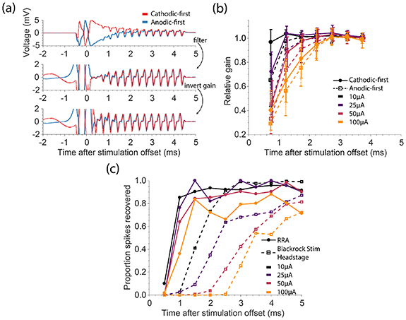
Figure 2. Evaluation of rapid-recovery amplifier (RRA). (a) Example recordings on the stimulated channel when evaluating the gain of the RRA are shown both before (top) and after (middle) acausal, time-reversed filtering, and after accounting for the changing gain (bottom). We stimulated with biphasic anodic-first (blue) or cathodic-first (red) pulses with phase duration of 200 μs, phases separated by 53 μs, and an amplitude of 50 µA. Pulses were simultaneously delivered on a remote channel to inject a 'known' signal. (b) The relative gain of the RRA for stimulation at different amplitudes. The gain was determined by measuring the peak-to-peak voltage of the injected signal. Error bars denote standard deviation across electrodes (n = 25). (c) Spikes were artificially added to artifact traces recorded on the stimulated channel. The proportion of simulated spikes recovered using our pipeline for both the RRA (solid lines) and the Blackrock Stim Headstage (dashed lines) across stimulation amplitudes (n = 10).
Download figure:
Standard image High-resolution imageWe tested the ability to recover spikes following stimulation by adding representative, naturally occurring spike waveforms to actual recordings of stimulation artifacts to establish a ground-truth reference. The proportion of these spikes that could be recovered with the Blackrock Headstage and with the RRA are shown in figure 2(c). We used logistic regression to predict the proportion of spikes recovered based on the stimulation amplitude and time after stimulation, (overall model χ2 = 1.97 × 10³, p
 0). Not surprisingly, spike recovery worsened with increasing stimulation amplitude regardless of amplifier (p
 0, t-test), but spikes were recovered at much shorter latencies with the RRA than with the Blackrock Stim Headstage (p
 0, t-test). The RRA also reduced the effect of amplitude (p = 0.0015, t-test) and increased the recovery rate (p = 0.0090, t-test).
3.2. Excitatory and inhibitory response to single pulses of ICMS
After evaluating the performance of the RRA, we used it for a series of experiments to quantify the neural responses evoked on the stimulated electrode. We first characterized the excitatory and inhibitory responses to single stimulus pulses across a wide range of current amplitudes (5–100 µA). Example raw and acausal filtered spikes for action potentials recorded at least 100 ms (top) and 1–3 ms after (bottom) stimulation offset are shown in figure 3(a). The shape of filtered spikes recorded shortly after stimulation was similar to those recorded long after stimulation offset. Responses for this example neuron are shown in figure 3(b). While it was not possible to record throughout stimulation (red shading indicates region obscured by the artifact), using the RRA allowed us to record many spikes that we could not have seen if we had used the Blackrock Headstage (grey shading). To quantify the amount of evoked activity, we measured the number of spikes evoked for each amplitude and subtracted the expected number of spikes due to baseline firing. The number of spikes evoked above baseline firing across amplitudes is shown in figure 3(c). The number increased significantly as amplitude increased (overall model F(30,223) = 4.88, p
 0; amplitude factor F(1,223) = 12.029, p = 6.3 × 10⁻⁴). Among the 29 out of 30 neurons that were activated with the range of currents tested, the median activation threshold was 10 µA (figure 3(c)).

Figure 3. Excitatory response on the stimulated channel after single pulses of stimulation. (a) Example spikes recorded on the stimulated electrode at least 100 ms after stimulation offset before and after acausal filtering. Spikes from the same neuron recorded 1–3 ms after stimulation offset before and after acausal filtering. (b) Response of the neuron in (a) to single cathodic-first pulses at different amplitudes. Each row is a different stimulation trial (728 total), and each tick represents an action potential from this neuron. Blue, horizontal lines separate stimulation trials at different amplitudes. Red shading depicts the time interval in which we were unable to record neural signals with the RRA. Grey shading depicts the corresponding time had we used the Blackrock Stim Headstage and Front-End amplifier. (c) The number of evoked spikes above baseline is shown across neurons (n = 30) for each stimulation amplitude. The box represents the 25th, 50th and 75th percentiles, whiskers represent the extent of the data, and X's mark outliers. (d) Distribution of activation thresholds across neurons. (e) The standard deviation of spike times within an evoked spike group is shown against the latency of that group for different stimulation amplitudes. (f) The number of groups evoked for different stimulation amplitudes. The number within each box and the shading of each box indicates the percentage of neurons. The prolonged artifact that occurred when stimulating with 100 µA likely obscured the entire initial group of spikes. When we determined that this occurred, we increased the group number by one (displayed in grey; 'adj').
Download figure:
Standard image High-resolution imageSufficiently high stimulation amplitudes evoked multiple spikes within 10 ms of stimulation offset. These spikes occurred at consistent latencies across trials, with later spikes having more varied timing than earlier ones. To quantify this, we grouped evoked spikes based on their latency (figure 3(b) and supplementary materials show example groups). Figure 3(e) shows the standard deviation of spike times within a group compared to the latency of that group for multiple stimulation amplitudes. This standard deviation increased significantly as group latency increased (overall model F(32,302) = 103, p
 0; latency factor F(1,302) = 574.13, p
 0). We also noticed that latencies decreased as stimulation amplitude increased, seen as a leftward shift in figure 3(a) as current increased to 100 µA, at which point the artifact likely obscured the first recorded group of evoked spikes. Using a linear model across all neurons, we determined that the latency of groups decreased by 3.6 ± 0.7 µs µA−1 as amplitude increased (overall model F(31,303) = 55.1, p
 0; amplitude factor F(1,303) = 25.497, p = 7.7 × 10⁻⁷).
The percentage of neurons that responded with different numbers of spike groups for stimulation at various amplitudes is shown in figure 3(f). For our example neuron, stimulation at 100 µA appeared to evoke 4 groups of spikes, as did 7% of neurons we recorded. However, at 100 µA, the extended artifact and decreased latency likely obscured the entire initial group of spikes, as can be seen in panel b. When we determined that this occurred, we increased the number of groups for the corresponding neuron by one (increasing the example neuron's group count from four to five in figure 3(f)). Even without this compensation, the number of groups increased significantly with stimulation amplitude (overall model: F(20,223) = 5.65, p
 0; amplitude factor: F(1,223) = 85.5, p
 0).
0).
Neuronal activity was typically suppressed anywhere from 10 to 150 ms after single pulses, depending on the stimulation amplitude (figure 4(a)). We fit a linear model to predict inhibition duration by amplitude across neurons (overall model F(30,180) = 1.9, p = 0.0057). We found that increasing stimulation amplitude significantly increased the inhibition duration (amplitude factor F(1,180) = 32.43, p = 5.0 × 10⁻⁸) and increased the fraction of cells undergoing inhibition (figure 4(b)). Stimulation amplitudes ⩾40 µA caused inhibition in ∼90% of neurons.

Figure 4. Inhibitory response recorded on the stimulated channel after single pulses of stimulation. (a) The inhibition duration across neurons (n = 30) recorded on the stimulated channel after single cathodic-first pulses of stimulation across stimulation amplitudes. (b) The fraction of cells with an inhibitory response is shown for each stimulation amplitude.
Download figure:
Standard image High-resolution image3.3. Temporal response to trains of ICMS
We hypothesized that the activity evoked by ICMS would decrease throughout long stimulus trains as a consequence of the long-lasting inhibition on stimulated electrodes following single pulses (figure 4). To test this, we stimulated on single electrodes with 4 s long trains at several amplitudes (20, 40, 60 µA) and frequencies (51, 80, 104, 131 Hz). Example spikes recorded from a neuron on the stimulated electrode are shown in figure 5(a) (grey) using the same format as figure 3(a). The mean responses across eight trains for nine of the 12 stimulation conditions are shown as grey traces in figure 5(b) for this example neuron. For this neuron, the evoked response rapidly decayed throughout the train, particularly for the larger amplitudes and frequencies. For the 21.5 ± 2.0 neurons that were activated significantly for each condition (Chi-Square test, α < 0.05), we computed a decay rate by fitting the firing rate during stimulation with an exponential (figure 5(c)). Using a linear model (F(26,231) = 14.7, p
 0), we determined that the evoked response decayed significantly faster with greater stimulation amplitude or frequency (amplitude: F(1,231) = 119, p
 0; frequency: F(1,231) = 134, p
 0). Increased frequency (amplitude) had a larger effect at higher amplitudes (frequencies) (interaction term: F(1,231) = 71.4, p
 0).
0).
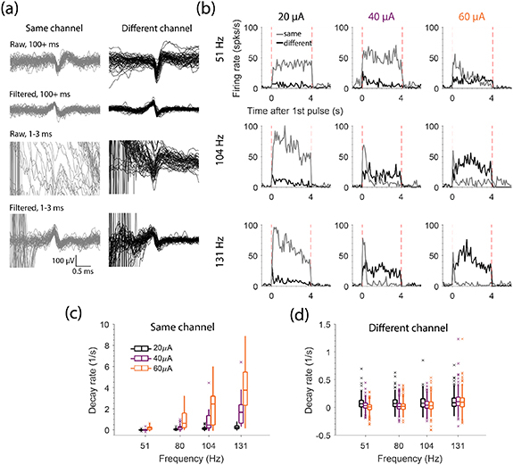
Figure 5. Evoked response throughout 4 s long trains of stimulation. (a) Example spikes for a neuron when the channel it was recorded on was stimulated (grey) and when a different channel was stimulated (black) in the same format as figure 3(a). (b) The mean firing rate across stimulation trials for the same neuron when the channel it was recorded on was stimulated (grey) and when a different channel was stimulated (black) for different stimulation amplitudes (columns) and frequencies (rows). Amplitudes and frequencies are noted above and to the right of the panels, respectively. Vertical, red dashed lines indicate train onset and offset. (c) The decay rates across neurons recorded on the stimulated channel for each amplitude and frequency (n = 21.5 ± 2.0 across conditions). (d) The decay rates for each neuron recorded on non-stimulated channels (for each amplitude and frequency (n = 258 ± 86 across conditions). Note the smaller y-limits in (d) compared to (c).
Download figure:
Standard image High-resolution imageIf neurons recorded on non-stimulated electrodes were driven transsynaptically by neurons activated near the stimulated electrode, then we would expect to see a similar rapid decay in the evoked activity for neurons on non-stimulated electrodes. If, on the other hand, neurons even on distant electrodes are driven directly, their decay rate may differ from that of neurons recorded on the stimulated electrode. To determine this, we examined the neuronal activity evoked on non-stimulated electrodes. Example spikes are shown for an example neuron in response to same- (gray traces) and different- (black traces) channel stimulation (figure 5(a)). In contrast to its response on the stimulated electrode, the activity of this neuron did not decay appreciably when a different electrode was stimulated (figure 5(b), black traces). The 260 ± 90 neurons recorded on non-stimulated electrodes that were activated by stimulation (Chi-Square test, α < 0.5) all had maintained responses throughout the stimulation train, as summarized in figure 5(d). Using a linear model with data aggregated across amplitudes and frequencies (overall model: F(81,3269) = 51.6, p
 0), we determined that the evoked response decayed significantly faster for neurons recorded on the stimulated channel than on non-stimulated channels (stimulated channel factor: F(1,3269) = 980.3, p
 0). These results imply that the response on non-stimulated electrodes is driven directly, or by evoked activity that occurs before we can record it.
After the end of an ICMS train, we expected neurons on the stimulated electrode to be inhibited for many milliseconds, as we observed with single pulses (figure 4). Indeed, low-frequency, 50 µA trains delivered for ∼0.2 s caused inhibition (see example in figure 6(a)) in about 50% of neurons, lasting from 10 to 250 ms (figure 6(b)). Faster stimulus frequency increased inhibition duration (Model: F(19,21) = 6.38, p = 5.9 × 10⁻⁵, frequency factor F(1,21) = 36.0, p = 6.0 × 10⁻⁶) but this effect was not observed in all 16 tested neurons. At 179 Hz, the highest frequency we tested, the fraction of cells with an inhibitory response was only ∼8%. Instead of inhibition in these cases, we observed a large burst of activity immediately after the stimulation train. This rebound excitation occurred for 75% of cells following stimulation at 179 Hz and lasted from ∼25 to 240 ms (figure 6(c)). If a neuron exhibited rebound excitation for multiple stimulation frequencies, higher frequencies almost always resulted in longer lasting rebound. During the longer 4 s trains, we observed rebound excitation very infrequently (2/25 cells) potentially because of the longer train duration.
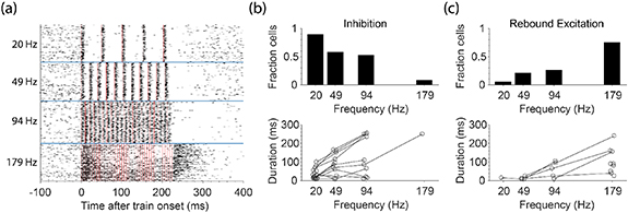
Figure 6. Rebound excitation recorded on the stimulated electrode after short trains of stimulation. (a) The response of an example neuron recorded on the stimulated electrode during ∼200 ms trains at different frequencies. Red lines indicate stimulation pulses. Stimulation frequencies are shown on the left of the figure for 50 µA stimulation. (b) The fraction of cells (n = 19 for 20, 49, and 94 Hz; n = 12 for 179 Hz) that displayed an inhibitory response after the end of the short trains (top) and the duration of the inhibitory responses (bottom) for each frequency. (c) The fraction of cells that displayed rebound excitation (top) and the duration of the rebound excitation (bottom) for each frequency. Lines connecting points represent data from the same neuron.
Download figure:
Standard image High-resolution image3.4. Spatial pattern of the response to ICMS trains
Both increased amplitude and frequency typically increase ICMS detectability, perhaps because of increased charge delivery (Otto et al
2005, Kim et al
2015, Sombeck and Miller 2019). Increasing amplitude leads both to more activity near the stimulated electrode (figure 3) as well as a wider spread of activity recorded across a multi-electrode array (Stoney et al
1968, Hao et al
2016, Kumaravelu et al
2022), likely because increased amplitude results in more charge delivered per pulse. Greater frequency, though, does not change the charge per pulse and thus may not lead to equivalent effects. To study these effects, we measured activity on non-stimulated electrodes throughout 4 s trains of continuous stimulation. We computed the mean firing rate above baseline for each neuron and amplitude/frequency combination across eight trains. Figure 7(a) shows the mean firing rate above baseline for each stimulation electrode aggregated across two monkeys against distance from the stimulated electrode. For each stimulation electrode, we only analyzed neurons that had activation thresholds at or below 20 µA when stimulating at 51 Hz. The evoked activity per pulse at 60 µA was significantly larger than that at 20 µA for 290 out of 437 neurons (p < 0.001, Wilcoxon rank-sum test) (figure 7(b)). Using a linear model (overall model: F(1251,362) = 19.4, p
 0), we determined that increasing amplitude and frequency increased the evoked firing rate (amplitude factor: F(11,362) = 674, p
 0, frequency factor: F(11,362) = 472, p
 0).
0).

Figure 7. Evoked response on non-stimulated channels during 4 s long trains of ICMS. (a) The firing rate above baseline against distance from the stimulated electrode for different amplitudes (columns) and frequencies (rows). Each point represents a neuron and stimulated electrode pair (n = 258.2 ± 86.1 across conditions). (b) The firing rate above baseline for each frequency and amplitude condition for responsive neurons. (c) The variance of the firing rate across trains for each condition. (d) The proportion of neurons activated at different distances is shown for a subset of amplitudes (color) and frequencies (line-style) (437 total neurons).
Download figure:
Standard image High-resolution image
We wondered whether the effect of frequency was simply due to the different number of stimulation pulses in the train. To analyze this, we normalized firing rates by the number of pulses and repeated our statistics (overall model: F(1251,362) = 20.9, p
 0). Increasing frequency no longer significantly increased the evoked activity per pulse (frequency factor: F(11,362) = 0.81, p = 0.37). The apparent effect of frequency was only due to the greater number of pulses in the train.
Neural discharge typically has a fixed FANO factor, meaning that the variance of the firing rate increases with the mean rate (Tolhurst et al
1983, Softky and Koch 1993). We wondered whether the variance of ICMS-induced neural activity also increases with amplitude and frequency, along with increases in mean rate (figure 7(b)). To test this, we measured the variance in firing rate across trains for each neuron and each condition (figure 7(c)). We observed no appreciable change in the variance with increasing amplitude and only a slight increase with frequency. To quantify these effects, we used a linear model to determine the effect of amplitude and frequency on the variance in firing rate (overall model: F(126,1362) = 7.21, p
 0). While increasing amplitude significantly decreased variance (amplitude factor: F(11,362) = 34.0, p =
  ) and increasing frequency increased variance (F(11,362) = 34.4, p =
  ), the effect sizes for both factors were tiny. This implies that ICMS-evoked activity does not have a fixed FANO factor; increasing either amplitude or frequency increases the mean rate without an equivalent effect on variance.
We also hypothesized that increased stimulation amplitude would increase the distance at which neurons are activated while increased frequency would not. Data for a subset of stimulation conditions are shown in figure 7(d). We used logistic regression to determine the effect of amplitude, frequency, and distance on the proportion of activated neurons (overall model χ2(104) = 1.69 × 10³, p
 0). Neurons were activated more diffusely at greater distances, an effect that was reduced by either increased current or frequency (both effects p ≅ 0). However, this interaction effect was much smaller between distance and frequency, effectively allowing current to control activation volume and frequency the proportion of activation.
4. Discussion
We developed hardware and software tools to enable recording at short latency after ICMS. With these tools, we were able to record roughly 0.7 ms after the end of stimulation, even from the stimulated channel. We investigated the evoked response to single pulses, and short and long trains of ICMS of varying amplitude and frequency to better understand the neural response to stimulation. Here, we compare our methods and results to those of previous studies, discuss the mode of activation for the spikes we recorded, and how our results may impact the design of biomimetic stimulation patterns in afferent interfaces.
4.1. Comparison of artifact suppression to previous techniques
Recording neurophysiological potentials immediately after passing current through an electrode is difficult; the large shock artifact typically prevents recordings for many milliseconds. We developed and evaluated the RRA to enable short latency recordings, particularly on the stimulated electrode. The RRA clamps the voltage below that which would saturate downstream electronics by reducing gain as the magnitude of the input voltage increases (figure 2(b)). An alternative approach to shorten the duration of the artifact is to electrically disconnect the recording system during stimulation (Zhou et al 2018). While this approach is effective on non-stimulated electrodes (Hao et al 2016), it cannot remove artifact on the stimulated electrode, which is caused by residual polarization of the electrode itself (Venkatraman et al 2008). Our approach is similar to clamping the slew rate (first derivative) of a signal, as has been done previously (Epstein 1995). By reducing the gain, we reduced the size of the artifact and prevented saturation, thereby allowing us to record at earlier latencies. Another important advantage of the RRA is the wide input voltage range (±15 V) that avoids the need for input clamping and stimulus current shunting of the relatively high voltage (<10 V) stimulus pulses. A benefit of our approach is that the RRA can be placed in front of pre-existing recording systems, in our case, the Cerebus system from Blackrock Neurotech. Saturation can also be prevented by using an amplifier with a lower gain and/or an amplifier with a higher maximum input voltage (Rolston et al 2009, Jung et al 2018).
While the RRA prevents amplifier saturation that would otherwise be caused by the large shock artifact, the recorded signal still returns only slowly to baseline after stimulation (figure 1(a)). This slow return is likely caused by slow dissipation of the residual charge on the electrode (Zhou et al 2018). To remove excess charge more quickly, custom electronics could be designed to actively discharge the electrode to a pre-stimulus voltage (Freeman 1971, DeMichele and Troyk 2003, Brown et al 2008), although this may introduce switching artifacts that diminish the effectiveness of this approach.
The slow return to baseline can also be removed offline. When done with a high-pass filter, it is important not to filter through the shock artifact, as this can cause ringing and obscure the neural signal. Some solutions include filtering the data beginning a fixed time after the end of stimulation (Hao et al 2016) or blanking the signal and using a low-order filter to limit ringing (Weiss et al 2018). Instead, we filtered acausally, backwards in time so that any ringing would be pushed before the stimulation, leaving the post-stimulus data clean (such acausally displaced ringing can be seen before 0 ms in figure 1(c)). This approach does not require defining a time at which the shock artifact has ended, though it does push neural signal back in time ∼100 µs. We compensated for this time shift by adjusting the time stamps of recorded spikes by 100 µs. With the RRA and acausal, time-reversed filtering, we were able to record ∼0.7 ms after stimulation offset, even on the stimulated electrode (figure 2(c)), revealing spikes that we could not have recorded with the Blackrock Stim Headstage (grey shading in figure 3(b)).
4.2. Mode of activation of recorded spikes on stimulated and non-stimulated channels
ICMS can evoke action potentials both directly and transsynaptically (Tehovnik et al 2006). Directly evoked spikes occur because stimulation changes the membrane potential of cells near the electrode, causing them to fire. Action potentials are typically initiated in axons, which have a higher density of sodium channels than do somas, resulting in lower activation thresholds (Nowak and Bullier 1998a, 1998b, Tehovnik et al 2006). Action potentials then propagate antidromically to the cell bodies and orthodromically to presynaptic terminals, where they may elicit further activity transsynaptically.
We wondered whether the spikes we recorded on the stimulated electrode were evoked directly, at either the axon or soma, or transsynaptically. Since we have no direct way of testing this, we inferred the mode of activation from the latency of evoked spikes. When we calculated the latest these spikes could occur, we assumed that directly evoked spikes were generated at the end of the cathodic phase (Stoney et al 1968, Jankowska et al 1975, Gustafsson and Jankowska 1976), although spikes may occur earlier in the stimulus pulse at higher amplitudes (such a shift is evident in figure 3(b)). We may actually observe these spikes somewhat later since they need to propagate from the site of initiation back to the soma. We estimated this potential antidromic distance and latency by first estimating how far spike initiation could have occurred from the stimulated electrode. To do so, we used Stoney's square-root relationship (Stoney et al 1968):

With  = 1292 µA mm−2 and
  = 10 µA, the median activation threshold of neurons in our study (figure 3(c)), the maximum spike initiation distance is ∼100 µm. Since somas can be recorded up to ∼150 µm from the recording electrode (Maynard et al
1997), the maximum distance an action potential could travel before being recorded is ∼250 µm. With a propagation speed of 1 µm µs−1 (Swadlow 1990), the maximum latency at which we expect to see a directly evoked spike is 0.25 ms after the end of the cathodic phase, (coincident with the end of the biphasic pulses). Hence, the earliest spikes we were able to see on the stimulated electrode, (0.7 ms after the end of the biphasic pulses; figure 3(d)), could not have been directly evoked.
= 10 µA, the median activation threshold of neurons in our study (figure 3(c)), the maximum spike initiation distance is ∼100 µm. Since somas can be recorded up to ∼150 µm from the recording electrode (Maynard et al
1997), the maximum distance an action potential could travel before being recorded is ∼250 µm. With a propagation speed of 1 µm µs−1 (Swadlow 1990), the maximum latency at which we expect to see a directly evoked spike is 0.25 ms after the end of the cathodic phase, (coincident with the end of the biphasic pulses). Hence, the earliest spikes we were able to see on the stimulated electrode, (0.7 ms after the end of the biphasic pulses; figure 3(d)), could not have been directly evoked.
Since the shortest synaptic delay is ∼0.4 ms (Gustafsson and Jankowska 1976), we estimate transsynaptic spikes could occur at a latency as short as 0.4 ms after the end of a biphasic pulse, similar to earlier estimates (Gustafsson and Jankowska 1976). This implies that the spikes we observed on the stimulated electrode were evoked transsynaptically.
We asked the same questions about the spikes recorded on non-stimulated electrodes. Due to the increased distance that evoked spikes could propagate, the latency at which we could record directly evoked spikes would also increase. For electrodes within 700 µm of the stimulated electrode, the maximum distance an action potential could travel is ∼950 µm. This makes the longest theoretical latency of directly evoked spikes ∼0.7 ms after the end of the biphasic pulses, very close to our observation. For these nearby electrodes, it remains likely we are recording transsynaptic activation.
4.3. Limitations due to missing directly evoked spikes
The major limitation of this study is that we were unable to record activity until ∼0.7 ms after stimulation offset, causing us to miss the initial, directly evoked spikes. To assess this impact, we estimated the proportion of spikes they represented. Since we can begin recording ∼0.7 ms after stimulation offset, we might miss at most one spike per pulse. In the worst case, where the neuron is directly activated by each pulse, 1.2–1.4 spikes are evoked per neuron across amplitudes (figure 3(c)). Thus the average of 0.2–0.4 transsynaptically evoked spikes we recorded accounts for 17%–30% of evoked spikes. Even though distance and amplitude affect the proportion of pulses which directly evoke a spike (Stoney et al 1968), we likely miss a large proportion of evoked spikes near the stimulated electrode.
While we cannot record directly evoked activity, we can infer something about its temporal pattern using activity recorded on non-stimulated channels, which must either be driven directly or transsynaptically by directly evoked spikes. Hence, we would expect the firing rate dynamics on non-stimulated channels to be like that of directly evoked spikes. Responses on non-stimulated channels were maintained throughout long trains of stimulation (figure 5), presumably driven by the maintained responses of at least some directly evoked neurons. In contrast, the likely-transsynaptic response recorded on the stimulated electrode decayed rapidly. It could be that directly evoked activity near the stimulated electrode decayed rapidly, but researchers using calcium imaging found that neurons closer to the stimulated electrode actually maintained their responses longer than those farther away (Michelson et al 2018). Instead, the decayed response we observed is likely caused by direct activation of local inhibitory neurons which competes with the excitatory effect (Overstreet et al 2013).
If the high temporal resolution that electrical recordings provide is not necessary, calcium imaging or voltage-sensitive dye imaging can be used to record activity during the stimulus pulse as these methods are not affected by the shock artifact (Histed et al 2009, Michelson et al 2018, Tanaka et al 2019). To isolate directly evoked spikes, pharmacological agents have been used to block synaptic transmission, enabling researchers to study the spatial pattern of directly evoked spikes (Histed et al 2009). Both that study and a more recent one using biophysical models (Kumaravelu et al 2022) concluded that ICMS activates a sparse and distributed population of neurons, likely due to local activation in axons propagating antidromically to somas. Combined with our results, we can describe the spatial and temporal pattern of directly and transsynaptically evoked activity.
4.4. Qualitatively similar evoked responses are observed across different experimental conditions
Across many studies using different levels of anesthesia, animal models, and recording techniques, the evoked response to ICMS is qualitatively similar. After stimulation, neurons exhibit short-latency excitation due to direct or transsynaptic activation (Tehovnik et al 2006, Margalit and Slovin 2018). We observed an increase in the amount of evoked activity from activated neurons and an increase in the spread of evoked activity with increasing amplitude (figure 3), consistent with previous observations (Butovas and Schwarz 2003, Hao et al 2016). With increased frequency, we observed a small increase in the amount of evoked activity per pulse, an effect that is further amplified by the increased number of pulses (figure 7). After short-latency excitation, neural activity is typically suppressed for long periods, an effect likely mediated by GABAB receptors (Butovas et al 2006). The duration of this long-lasting inhibition increased with amplitude in our study (figure 4), in contrast to previous reports of no such increase for neurons recorded farther from the stimulated electrode (Butovas and Schwarz 2003). After inhibition, we often saw a large increase in firing rate (figure 6) (Butovas and Schwarz 2003). This rebound excitation may be due to recurrent excitation within cortical circuits, mediated by calcium channels (Molineux et al 2006, McElvain et al 2010). Throughout trains of stimulation, we observed a rapid decay of the transynaptically evoked activity recorded near the stimulated electrode (figure 5), similar to previous observations (Michelson et al 2018).
4.5. Implications for biomimetic stimulation patterns
In monkeys, stimulation in tactile cortices evokes sensations at locations corresponding to the receptive fields of neurons recorded on the stimulated electrode (Tabot et al 2013). Different temporal patterns of stimulation can be distinguished and used to convey useful information (Romo et al 1998, London et al 2008, Berg et al 2013, Dadarlat et al 2015, Callier et al 2020). Similar observations have been made in humans with tetraplegia and neuropathy (Salas et al 2018, Chandrasekaran et al 2021, Fifer et al 2020; Hughes et al 2021b), including the ability of one person to identify which of multiple fingers of a robotic hand, linked to somatosensory cortex (S1) stimulation, were touched (Flesher et al 2016). More recently, somatosensory ICMS was used to provide contact and pressure-related feedback, which improved a user's ability to control a robotic arm to reach and grasp (Flesher et al 2021). The stimulus parameters in this most recent example were quite simple, a linear mapping from index and middle finger joint torques to appropriate electrodes, and evoked sensations that were judged to be "possibly natural" (Flesher et al 2016). Biomimetic stimulation patterns, those that aim to evoke activity that mimics the spatial and temporal properties of naturally occurring activity, may be necessary to evoke more naturalistic sensations (Bensmaia and Miller 2014).
To develop biomimetic stimulus patterns, it may be useful to compare the spatial and temporal dynamics of naturally occurring activity to the activity evoked by stimulation. In tactile areas, neurons respond to skin indentation with a large transient response and smaller sustained response (Callier et al 2019). Our data suggest that neurons entrain their responses to each pulse in the train. Thus, to recreate the temporal dynamics of this response, the frequency of stimulation needs to be modified throughout the train. In proprioceptive areas, limb movements evoke a complicated spatiotemporal pattern of activity across cortex that is dependent on the direction and speed of reaching movements, as well as interaction forces (Prud'homme and Kalaska 1994, London and Miller 2012). Recreating these patterns may require small amplitudes on many electrodes, in order to target groups of neurons with sufficiently similar encoding properties (Weber et al 2011). Even with small amplitudes, though, some directly activated neurons may be located far from the stimulated electrode due to the local activation of axons (Histed et al 2009, Kumaravelu et al 2022). Monitoring the locations of activated neurons may enable researchers to design stimulation patterns that more closely mimic the naturalistic spatial response more closely.
The activity evoked by ICMS is also unnaturally synchronous across neurons. There are several stimulus protocols that may serve to reduce synchrony, including stimulating with amplitudes nearer the activation threshold, where spikes are not evoked reliably (figures 3(b) and (d)). Alternatively, single pulses within a train can be replaced with kilohertz bursts of pulses, with amplitude increasing throughout the burst (Formento et al 2020). Neurons with different activation thresholds will be activated at different times during the burst. Finally, multi-electrode stimulation could be delivered asynchronously across electrodes. The ability to record the evoked activity would allow the efficacy of any combination of these approaches to be evaluated.
4.6. Linking evoked activity to sensation
Most sensory modalities obey Weber's law: The just noticeable difference (JND) in stimulus intensity increases with increased amplitude (Ekman 1959). This log-like relation likely occurs because the firing rate variance increases with mean firing rate (Johnson 1980a, 1980b). As a consequence, it is possible to detect very small differences within natural low-intensity stimuli. In contrast, for ICMS stimulation, the JND remains constant across amplitudes and frequencies (Kim et al 2015), potentially limiting the discriminability of small inputs, and the total number of discrete intensities that can be discriminated. While we recorded a linear increase in mean firing rate with increased amplitude and frequency, there was little change in the variance as these parameters changed (figure 7), likely the source of the JND that is unchanging with increased stimulus intensity.
In our experiments, we typically recorded a maintained response on non-stimulated channels throughout 4 s long trains (figure 5), a response which likely reflects the temporal dynamics of directly evoked spikes. Because of this, we would predict the perceived intensity due to longer trains to be constant for at least this length of time at the frequencies and amplitudes we tested. Our observation is consistent with the observations of a human participant in a recent study, who reported constant perceptual intensity for ∼7 s (Hughes et al 2021).
However, after the end of long stimulus trains, the evoked sensation described above did not disappear immediately, but persisted for a couple of seconds. We often observed a large burst of rebound excitation after the end of high frequency trains (figure 6), which could potentially lead to persistent sensations. Since rebound excitation primarily occurred at high stimulation frequencies, it may be that there is a maximum frequency that future afferent interfaces can use to avoid the effect.
4.7. Online recording in the presence of stimulation artifact
For most applications, afferent interfaces would only be useful when combined with an efferent interface, thereby providing both restored somatosensation and movement (O'Doherty et al 2011, Flesher et al 2021). However, stimulation in S1 produces large artifacts in recordings from motor cortex (M1). With causal filters, neural signals can be recorded from M1 in a human ∼0.7 ms after offset of stimulation applied in S1. At low stimulation frequencies, losing the ability to record from M1 for short periods after each pulse may not have much of an impact on decoding performance. When intended cursor velocity was decoded from M1, artificially dropping a random 20% of M1 signals caused only a 10% decrease in decoder performance (figure 8 in (Young et al 2018)). While acausal, time-reversed filtering may allow for slightly earlier recordings, the increased amount of data would likely have a negligible impact on decoding performance.
However, as stimulation protocols become more complicated, with stimulation at high rates and on many electrodes (Bensmaia and Miller 2014, Sombeck and Miller 2019), the percentage of time in which signals can be recorded from M1 will decrease, further decreasing decoder performance. Stimulation at 333 Hz, either on a single electrode or distributed across electrodes, would result in 50% loss of signal, assuming a total blanking duration of 1.5 ms per pulse (Weiss et al 2018). With some non-trivial amplifier modifications to increase the gain during the stimulus artifact above zero, the RRA could potentially enable neural recordings even during the stimulus pulse, albeit at a much reduced gain from those of usual recordings. Although we did not explore them here, there are numerous approaches that could be used to extract neural signal from the artifact if the recorded signal is not saturated: adaptive filtering (Nag et al 2015, Mendrela et al 2016), template subtraction (Hashimoto et al 2002, Montgomery Jr, Gale, and Huang 2005), independent component analysis (Hyvärinen and Oja 2000, Lemm et al 2006), linear regression (Young et al 2018), and deep neural networks (Zhang and Yu 2018, Tamada et al 2020). Of particular note is ERAASR, a technique which uses principal component analysis to exploit the similar structure of the shock artifact sequentially across electrodes, pulses, and then trials (O'Shea and Shenoy 2017). With these approaches, it may be possible to recover neural signal throughout multi-channel stimulation, thereby enabling full band-width recordings in M1 while providing somatosensory feedback via ICMS in S1. Such technology will likely be necessary to accurately decode motor intent as ICMS feedback becomes more complicated.
Data availability statement
The data that support the findings of this study are available upon reasonable request from the authors.
Acknowledgments
We would like to thank Tucker Tomlinson and the rest of the Miller Limb Lab for useful discussions that greatly improved this work. This research was funded by National Institute of Neurological Disorders and Stroke Award No. NS095251 and No. F31NS115478, and by National Institute of Health Grant No. T32HD07418. The content is solely the responsibility of the authors and does not necessarily represent the official views of the National Institutes of Health.