

Abstract
While conventional shock tubes have a distinct advantage in dynamic calibration methods due to their inherent capability to generate pressure pulses of desired amplitude and fast rise time, they are limited to the lower levels of the pressure amplitude realization range (≤7 MPa). With the increasing need for a traceable dynamic calibration standard across wider pressure ranges, a novel technique using converging shock waves is demonstrated in this work that pushes the upper limit of the standard shock tube into the medium-high pressure range. The experiments are conducted in the shock tube facility equipped with a test section that smoothly transforms the incident plane shock into a spherical shock wave that converges, accelerates and thereby amplifies its strength many folds. The experimentally recorded pressure traces are compared with numerical simulations performed by an in-house code. Using this technique, pressure pulses with peak amplitudes in the range of 30–40 MPa, with  3.4% uncertainty based on numerical reference profile, were realized in the test section with nominal usage of resources.
Export citation and abstract BibTeX RIS

Original content from this work may be used under the terms of the Creative Commons Attribution 3.0 license. Any further distribution of this work must maintain attribution to the author(s) and the title of the work, journal citation and DOI.
1. Introduction
Time-dependent pressure is an important quantity to be measured in a wide variety of fields like aerospace, astronautics, combustion analysis, turbomachinery, production industry, explosion safety and ballistics [1–6]. Generally, commercially available pressure sensors are used in the tracing of the dynamic character of pressure at the target area. There is a wide variety of sensors that meets the demand in terms of pressure amplitude range and frequency response. In many cases, these sensors are calibrated statically as there is no traceable universal standard for dynamic measurement of pressure [7]. While static calibration has been well developed with promising traceability and accuracy, using them for dynamic measurement of pressure leaves an uncertainty over the reliability of the measured data warranting a traceable dynamic standard to be established [8–10]. The difficulty in dynamic calibration comes with the challenges to generate well-defined pressure changes of the required rate and amplitude. In most cases, a reference pressure transducer calibrated elsewhere is also engaged.
Among the few available dynamic calibration methods [7, 11], the most notable are the shock tube [12, 13] and the drop weight [14, 15] methods. Both are aperiodic single pressure pulse generators. Shock tube, in particular, is a device generating a moving shock wave of desired strength, which forms a rapid pressure step once it reflects from the shock tube end wall. The amplitude of such a step can be analytically calculated using well-known conservation equations. The rise time of the pressure change is of the order of a few hundred nanoseconds and the duration of the step is generally of the order of a few milliseconds (dependent on the shock tube dimensions). As will be shown in section II of this work, the drawback of this approach is the generation of a relatively low pressure step amplitude - in the range below 7 MPa for nominal operations. These can be pushed further up to about 10–15 MPa, but that requires large amount of resources and strong materials to be used in the construction of the facility leading to very high operating costs. Any further increase in pressure beyond a certain limit is in fact impossible using conventional shock tubes despite the availability of sufficient resources. On the other hand, the drop weight method can generate pressure pulses with significantly higher amplitudes (30–400 MPa), however, this technique suffers from increasing uncertainties for lower level pressure range measurements. Evidently there exists a gap in the range of 7–40 MPa that needs to be overlapped and bridged either by increasing the upper pressure limits of shock tubes or by lowering the range of reliable pressure estimations in drop weight methods. One should note that this overlapping range is of importance in various applications, e.g. in internal combustion engines [16], where reliable dynamic measurement of in-cylinder pressure (in the discussed overlapping range) is needed for understanding the combustion processes allowing for engine optimization and fuel consumption.
Since shock tube approach is one of the promising dynamic calibration methods available, negating its aforementioned drawbacks can lead to substantial development in the realm of dynamic pressure standards. With that being the motivation, this paper focuses on a novel technique of using converging shock waves, that pushes the pressure realization in a modified shock tube upwards to the range of 40 MPa with nominal resources. An in-house numerical code predicting the transient pressure profile has been developed and validated using previous and current data from experiments. Industrially available sensors are used in the experimental pressure measurements and the results are discussed based on its comparison with the numerical predictions. This work is a partial contribution within EMPIR project [17] dealing with development of measurement and calibration techniques for dynamic pressures and temperatures (17IND07, DynPT).
2. Basic shock tube theory
A shock tube is a device used for generating shock waves in a controlled laboratory environment. Figure 1(a) illustrates the initial state of the conventional shock tube, where it is divided into two chambers exposed to two initially different pressures: low pressure chamber, usually called driven section (region 1) and high pressure chamber, usually called driver section (region 4). When the separation between the driver and driven sections is instantaneously removed, a series of compression waves are generated within the driven gas which later coalesce to form a shock wave that propagates through the driven section with velocities exceeding the local speed of sound. Figure 1(b) illustrates position (x) vs time (t) diagram of the processes developing inside the shock tube after the flow initiation. A shock wave travelling into the undisturbed gas (region 1) is a discontinuity across which the thermodynamic flow properties like pressure (P), velocity (v), density (ρ) and temperature (T) rise abruptly (region 2). A contact surface follows the shock front into the driven section separating the driven gas (region 2) and the driver gas (region 3). An expansion fan centered at the separation position is also generated to release the pressure in the driver section. Once the incident shock wave reaches the shock tube end-wall, it reflects and travels back thereby abruptly increasing the pressure and other corresponding thermodynamic properties once again (region 5). It is well-known that for a calorically and thermally perfect gas, the ratio of uniform properties across the shock wave can be determined by solving the equations of mass, momentum and energy conservation across the shock front (known as Rankine-Hugoniot relations, for more detailed derivation see e.g. [18]). Assuming initial thermal equilibrium of the driven/driver gases, the following expression can be obtained between the pressure ratio across the initial separation,  , and the incident shock wave Mach number, Ms [19]:

Figure 1. Position (x) vs time (t) diagram depicting the conditions in a uniform section shock tube.
Download figure:
Standard image High-resolution image
where Ms is defined as  ; us is the speed of the shock front; a1 and a4 are the speeds of sound of the driven/driver gas; and γ1 and γ4 denote the adiabatic indices of the driven/driver gas accordingly. Equation (1) implies that the ratio is dependent only on the strength of the incident shock wave and the type of the driven/driver gases.
Figure 2(a) shows the corresponding variation of Ms with  for various driver and driven gas combinations. It can be easily seen that for all gas combinations the larger the pressure ratio, the stronger is the incident shock wave, which in turn results in higher pressure ratio across the shock wave. However, Ms tends towards some asymptotic value for higher ratios of
  . The maximum attainable Ms at infinite initial pressure ratio for any gas combination can be calculated using the following expression (deduced from equation (1)):
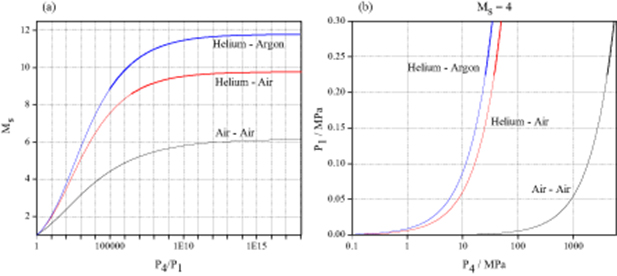
Figure 2. For different gas combinations, (a) the driver/driven pressure ratio required to generate a shock wave of desired strength, Ms; and (b) the pressure to be set for obtaining Ms = 4 shock wave when either the driver or driven pressure is fixed.
Download figure:
Standard image High-resolution imageOnce the shock wave reflects off the end wall in the driven section, the derivation of the Rankine-Hugoniot relations can be continued, which results in the following pressure ratio,  :
:
Evidently P5 is also a function of the incident shock Mach number, Ms, and represents the maximum possible pressure step amplitude obtained in the entire setup. Generally obtaining large pressure ratios are challenged by existing vacuum technologies for the driven section, as well as the material strength of the driver section and the separation opening mechanisms. For instance, the pressures required in both the sections for obtaining the incident shock wave Mach number Ms = 4 is demonstrated in figure 2(b). If the driven section conditions are fixed at atmospheric pressure (P1 = 0.1 MPa), pressure in excess of 10 MPa is required in the driver and it increases even more when the losses incurred during the opening of the separation region are taken into account. Obviously P4 can be reduced by dropping down the driven pressure P1, however that results in a correspondingly lower P5. This can be easily shown by solving equation (3) with Ms = 4 giving  . By setting P1 with 0.01 MPa as opposed to e.g. 0.1 MPa, the pressure value P5 would be 1.11 MPa rather than 11.1 MPa respectively. Since this work aims at reaching large end pressures, setting low P1 is not beneficial. On the other hand, for higher P1 larger driver pressures are necessary to maintain the same Mach number Ms. For comparison table 1 represents the calculated pressure amplitudes for an ideal shock tube run targeting Ms = 4 for various gas combinations at atmospheric conditions in the driven section (P1 = 0.1 MPa). It is clear that by matching gas characteristics the required driver pressure can be substantially reduced, however, figure 2(b) suggests that higher gains of the incident shock Mach number would still require unproportionate driver section resources.
3. Converging shock wave (CSW)
As shown in section 2, large amounts of resources are required to generate high pressures in a conventional shock tube of uniform cross-section area. However, shock waves are associated with high initial energy densities distributed within its thin streak. By converging the shock wave through smooth area reduction techniques, its energy density per unit length increases due to energy conservation followed by acceleration of the shock front thereby increasing its strength (Ms). This process is accompanied by the transformation of the initially plane shock front into a spherical shape [20, 21]. A schematic of the convergence process is as shown in figure 3. As the spherical shock front further converges, extreme conditions are created at its focal point by shock amplification. Liverts and Apazidis [22] reported that upon converging a plane incident shock wave of Ms = 4.5 from 80 mm diameter tube to 16 mm and thereafter to 0.6 mm resulted in a shock wave of Ms = 9 and 24 respectively. Since the thermodynamic properties are only dependent on Ms, CSWs provide a way to break through the limitations hindering the usage of uniform section shock tube beyond a certain pressure value.

Figure 3. Schematic of a plane shock transformation and convergence in a converging channel.
Download figure:
Standard image High-resolution image3.1. Experimental setup
The shock waves in this work are generated using the shock tube facility shown in figure 4(a). The driver and driven sections were made of cylindrical steel tubes separated by a fast opening valve (ISTA KB-80-50) with a pressure rating of 5 MPa and 7 ms stated opening time [23]. In order to provide sufficient length for shock formation, the driven section was made almost 4 m long with a uniform cross-section diameter of 80 mm. The driver section was relatively shorter measuring 0.7 m in length but with a variable diameter of 80–160 mm in order to retard reflection of the expansion waves from the driver end wall. Helium and argon were used as the driver and the driven gas respectively. Argon was chosen due to its monatomic gas properties enabling it to be considered as a perfect gas at relatively large shock Mach number  10 [22]. The speed of the shock wave was measured using two piezoelectric pressure sensors (PCB 113B24), S1 and S2, which were mounted 250 mm apart from each other at the far end of the driven section. For the initial conditions set in the experimental runs, the shock waves were always formed (confirmed from the step pressure profile measured by both sensors) before reaching sensor S1.

Figure 4. (a) Schematic of the shock tube facility along with the test section. (b) Close-up of the test section showing the transformation section (TS), conical section (CS) and sensor mount location.
Download figure:
Standard image High-resolution imageThe unique feature of this shock tube is the converging test section, consisting of a transformation section (TS) and a conical section (CS), immediately following the straight driven section. A close-up of the test section is shown in figure 4(b). The TS is a 270 mm long section whose diameter varies smoothly from 80 mm at the inlet to 16 mm at the outlet immediately followed by the axisymmetric conical CS. The shape of the TS transformation was parameterized as:
where 0 ≤ θ ≤ 0.35π, A = 300.7 mm, B = 40 mm and R = 57.3 mm. This shape was chosen after a series of calculation done by Kjellender et al [20, 21] fulfilling the condition that the shock foot remains normal to the wall without reflection/creation of Mach stem during its convergence. It can be scaled to any size provided its profile is preserved. In order to visually verify the nature of the shock structure along with the transformation, a scaled 2D version of the profile of length 150 mm and width 50 mm was printed in plastic using a 3D printer and tested in the exploding wire facility at KTH. The facility is a compact, 2D blast wave generator with visual access constructed within the group recently. The details on its construction, operation and the visualization systems can be found in [24], as it is beyond the scope of this work. Figure 5 shows the shadowgraph images captured in the facility. Due to the imaging limitations, only 100 mm × 35 mm of the 2D profile (from the smallest opening end) was optically captured and shown here. The dark line in the images is the shock front captured by the camera at two instants during it propagation through the profile. In figure 5(a), the shock front is very slightly curved as it is still in the early stages of the transformation process. The curvature increases along the length of the profile and the radial shock front is observed in figure 5(b). From the zoomed in view of the raw and processed image shown in figure 5(c) and (d) respectively, it can be confirmed that the shock front is in fact continuous (no Mach stem) with no reflection observed at the point of contact of the shock front and wall.

Figure 5. Shadowgraph images of the flow through the 2D TS profile. Note that due to the imaging limitations, only 100 mm × 35 mm of the 150 mm × 50 mm 2D profile is shown here. (a) Time instant when the incident shock entered the visual frame. (b) Image taken close to the profile end showing the converging shock wave. (c) Zoomed in view of the converging radial shock. (d) Processed image of (c) highlighting the shock wave.
Download figure:
Standard image High-resolution imageHowever, the TS for the shock tube was constructed by casting plastic around a CNC machined steel mold, as shown in figure 6(b). The cast was then housed in a steel tube with a flange which was attached to the shock tube (see TS in figure 6(a)). For the 3D case, extensive tests on the section performance were conducted by Kjellander et al [20, 21] (including the CS convergence up to 0.3 mm at the outlet). Therein, it was concluded that a spherical shock front was indeed propagating in accordance with the Guderley's self-similar convergent solution [25, 26]. Later, Liverts and Apazidis [22] included a study by replacing the CS with a pressure sensor mounted at the end of TS and directed towards the incident flow. Based on their results on time of shock arrival and pressure amplitude, it was verified that the initially plane shock front successfully transformed into a spherical shape at the TS exit. Also, extensive amount of data based on spectroscopic analysis in [20, 22] made on the current test section had negligible distortion, further substantiating the transformation and convergence of the shock wave, as otherwise, the acquired radiation would significantly deviate between different runs.

Figure 6. (a) Picture showing the end part of the shock tube assembly mounted with TS and CS. (b) The steel mold used for casting the TS along with its inner view. (c) Top and side view of the CS.
Download figure:
Standard image High-resolution imageKjellander [20] also reported that unstable oscillations in the shock shape occur at the vicinity of the focal point region of extremely large shock Mach numbers. Since one of the criteria was to not exceed shock Mach number 10 [22], such extreme conditions were deemed unnecessary. Besides, the diameter of the pressure sensor being used here is around 5.5 mm, inevitably cutting off the unnecessary oscillation range. Hence the CS was designed to vary from 16 mm at the inlet to 7 mm at the outlet with the cone half angle being 21°. The top and side view of the CS made of steel is shown in figure 6(c). The overall length of the test section was 288 mm. The reflected pressure profile (P5) of the converged 7 mm spherical shock wave was recorded by a piezoelectric pressure sensor S3 (PCB 113B23) mounted at the CS tip. Sensor S3 is stated to be capable of measuring pressures up to 68 MPa at a resonant frequency of 500 kHz. It is to be noted that the converging shock wave will impact the flat sensor face unevenly. However, as the largest distance occurring between the shock wave and the sensor was along the tube centerline with a value of around 0.5 mm (at the moment of first contact) and coupled with the fact that the speed of the shock wave was relatively higher, the uneven loading timescale was calculated to be well below the response time of the sensor.
The shock Mach number Ms was determined using time-of-flight method i.e by calculating the distance travelled to the time taken by the shock front to reach sensor S2 from S1. Calculating Ms was vital for analysis, based on decoupling the effects of initial conditions. Figure 7 shows the Ms obtained for the range of driver pressures used in this work when the driven pressure is fixed at 0.1 MPa. Note that a number of combinations of  can be used to get similar Ms. After a few initial tests, it was decided to maintain P1 at 0.1 MPa as, (1) it satisfied the design criteria of not exceeding the converging Ms = 10 limit; (b) it would serve as a starting point comparison for future research since the tests are done at atmospheric conditions; and (c) to provide sufficient safety factor for shock tube operation. Due to the accelerating nature of the shock front within the converging test section, the speed of the shock wave at the moment of impact cannot be registered, but nevertheless the time taken for it to travel from sensor S2 to S3, denoted as ΔtS2 − S3, is plotted against its corresponding initial Ms in figure 7(a). Following the impact at S3, the shock wave is reflected and it travels back towards S2. During this return propagation, the shock wave expands following the diverging nature of the section. The total time taken for the crossing of the incident shock and the reflected shock over sensor S2 (denoted as ΔtS2 − S3 − S2) i.e total time taken to travel from S2 to S3 and back to S2 is plotted against its corresponding initial Ms in figure 7(b). This plot is of importance in evaluating the effect of parameters like non-uniform shock reflection, boundary layer etc on shock deceleration in section 3.3. Since Ms is the ratio between the velocity of the shock wave (v) and the speed of sound (a), its associated standard uncertainty (uMs) based on the law of propagation of uncertainties (assuming uncorrelated input quantities) is:
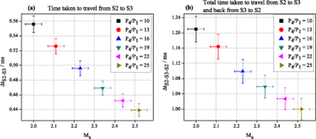
Figure 7. The shock Mach number, Ms, calculated through sensor S1 and S2 plotted against (a) the time taken for it to travel from sensor S2 to S3, ΔtS2 − S3; (b) total time taken to travel from S2 to S3 and back from S3 to S2, ΔtS2 − S3 − S2. P1 is fixed at 0.1 MPa.
Download figure:
Standard image High-resolution image
which leads to:
where uv and ua represent the standard uncertainties in velocity and speed of sound respectively. Both the quantities are expressed as:
where ud = 1.5 mm is the standard uncertainty associated with the distance between the sensors S1 and S2 (d = 250 mm); ut is the standard uncertainty associated with the time (t) between the corresponding sensors; uT is the standard uncertainty in resolution of the instrument measuring temperature (T); γ and R represent the ratio of specific heat and gas constant respectively.
The uncertainty ut has two components: type A evaluated from the data of six runs in the shock tube; and type B comprising of time accuracy and sampling interval of the oscilloscope, rise time of the sensors and its resolution limit. The losses arising at the Fast Opening Valve (FOV) can be different for each run due to the inconsistent opening of the valve along with the unavoidable small deviation in  . While designing the shock tube, the length of the driven section was intentionally made longer in order to provide sufficient time for shock formation. With that ensured, the only other possible effect is on the strength of resulting shock wave. Since this being the largest random error, it was evaluated implicitly through the six individual runs. The oscilloscope used in the experiments was a Tektronix TDS 2014C and the time accuracy was determined from the relation specified in the manual as ± (1 sample interval + 100 ppm (reading) + 0.6 ns). The stated sensor rise time was ≤ 1 µs and since the sensors have relatively high sensitivity value coupled with a strong shock passage, the uncertainty for triggering the sensor was insignificant compared to the other uncertainty sources. The least significant digit (LSD) of the sensor resolution in time was 1 µs. The assumed probability density distribution was rectangular for sources without manufacturer specification.
Similarly, the uncertainty in sensor pressure measurement (uP) comprises of the type A evaluation from six runs, sensor sensitivity, sensor resolution, LSD of the sensor and scope and driven pressure P1. While the stated sensitivity for both the sensors used in the measurement was ±10%, the resolution of sensor S2 was 35 × 10−6 MPa and that of sensor S3 was 280 × 10−6 MPa. The LSD of the sensor resolution in pressure was 1 × 10⁻³ MPa although the scope had higher LSD. The driven pressure P1 has a direct significance in pressure measurement as it is dependent on Ms and a flat multiplier over the sensor measured value. Although P1 is controlled by the computer automated to maintain the set value, small variations in pressure was unavoidable. In order to compensate for this effect, a reasonable estimate of ±0.02 MPa was applied to the mean value. A sample uncertainty budget for six runs with similar initial conditions expanded to a 95% level of confidence [using coverage factor (k) determined from BIPM,s JCGM 100:2008 based on the overall effective degrees of freedom (νeff) is given in table 2. Assuming sensitivity coefficient to be 1, νeff was calculated using the following Welch-Satterthwaite formula:
Table 2. Sample uncertainty budget for six runs.
| uncertainty | factor (k) | uncertainty | uncertainty | ||
| ΔtS1 − S2 (µs) | 392.6 | 2.1 | 2.1 | 4.4 | 1.1% |
| v (ms−1) | 637.8 | 5.2 | |||
| a (ms−1) | 319.8 | 0.1 | |||
| Ms | 2 | 0.02 | 2 | 0.04 | 2% |
| ΔtS2 − S3 (µs) | 558 | 5.2 | 2.31 | 12 | 2.15% |
| ΔtS2 − S3 − S2 (µs) | 1235 | 14.8 | 2.36 | 35 | 2.8% |
| P2 (MPa) | 0.46 | 0.027 | 2 | 0.055 | 12% |
| P5 (MPa) | 15.2 | 0.92 | 2 | 1.84 | 12.1% |
where uc(y) is the combined uncertainty which in here represents ut and up;  and νi are the individual uncertainties and their respective degrees of freedom which represents the components used in estimating ut and up. For estimating the expanded uncertainty of Ms, k = 2 was used.
3.2. Experimental pressure profile
The discussion in this section is based on the measurement made by the pressure sensors. A sample pressure profile traced by the sensors S1–S3 for a helium-argon gas composition is as shown in figure 8. The driver and driven pressures were 2.5 and 0.1 MPa respectively. The step profiles recorded by sensors S1 and S2 confirmed that the shock wave was formed and the corresponding shock Mach number was measured to be 2.52 using both time of arrival method and from the measured pressure amplitude. The shock front was then transformed into a spherical form in the TS and further converged in the CS thereby increasing its strength manyfold. The reflected pressure profile as recorded by S3 is shown in figure 8. The peak pressure (pressure value at the highest point in the S3 profile) was measured to be 32 MPa using curve fitting method near the peak. To put things into perspective, for Ms = 2.52 in a straight section, the maximum peak pressure that would be attained is only 3 MPa. Looking from another angle, obtaining 32 MPa peak pressure in a straight section would require Ms = 6.8 shock wave which in turn requires 245 MPa driver pressure - an unrealistic value. It is to be noted that although the strength of the shock has been amplified due to the converging mechanism, it comes at the expense of a shorter time duration of the peak pressure. On a positive note, this generates a pressure profile consisting of both a rising and falling phase covering the true operating conditions of the sensor.
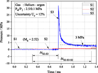
Figure 8. Experimental pressure profile recorded by the sensors S1, S2 and S3 for a helium-argon gas combination. It is to be noted that the step profile measured by S1 and S2 was that of P2 while S3 measured the P5 pressure profile. The profile is estimated with an uncertainty of 12%.
Download figure:
Standard image High-resolution imageA systematic series of experiments with different Ms (while maintaining P1 at 0.1 MPa) were conducted in order to cover an applicable range. Figure 9 plots the peak pressures measured at S3 as a function of Ms. Even for the lowest initial shock Mach number Ms = 2 obtained in the study, the converging cone was able to induce peak pressures of approximately 15 MPa, thereby easily surpassing the limits of conventional shock tubes.
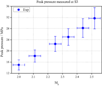
Figure 9. Experimental peak pressures measured at S3 as a function of Ms.
Download figure:
Standard image High-resolution image3.3. Numerical analysis
Numerical analysis plays an important role in this paper for two reasons, viz, (a) to better understand the properties of the incident shock wave during its convergence in the test section; and (b) to compare and validate the experimental results obtained from the sensors. The numerical simulations were performed using an in-house code that was developed to solve the full set of compressible Euler equations using Artificial Upstream Flux Vector Splitting Scheme (AUFS). The equations were essentially reduced to one-dimensional form along with a geometric source term accounting for spherical symmetry. The basic idea of the scheme is to split the flux vector using artificial wave speeds that adjust the direction of wave propagation [27]. The numerical scheme has been tried, tested and validated on a variety of problems, with it consistently demonstrating good accuracy [22, 28–31]. The axisymmetric version of the code has been specifically utilized to study spherical implosion shocks [22] where it was validated against experimental data.
Mesh independency study for the current problem with Ms = 2 and 2.52 was conducted and the results are as shown in figure 10. In figure 10(a) and (c), the study also performed another role of verifying the scheme by comparing the predicted value with theory and step-function based experimental data from sensor S2. The cell size was uniformly distributed in the region prior to the test section and was gradually decreased upon approaching the CS with the lowest cell size found adjacent to location S3. For simplicity of discussion, the meshes were categorised into coarse, medium, fine and very fine where the cell sizes were - in the order of highest/lowest (in mm) - 2.3/1.1, 1.5/0.7, 0.7/0.3, 0.3/0.1, 0.15/0.07, 0.03/0.01 and 0.015/0.007. Deviation from analytical value as well as between each other was observed for coarse and medium meshes. Upon further refining to fine meshes, the numerical solution showed accurate alignment with theory and close agreement with the mean experimental value. Running the simulation with very fine meshes did not yield any change as the solution stagnated following fine mesh thereby becoming grid independent solution. This also confirms the accuracy of the simulation when juxtaposed with theory and experimental values. Similar trend followed for numerical estimation at location S3 in figure 10(b), where moving from coarse to fine (for Ms = 2) or very fine (Ms = 2.52) resulted in mesh independent solution. However significant deviation from experimental value, even beyond the calculated uncertainty, was observed with no analytical solution available to compare it against. The numerically estimated Mach number at location S3 was around 5.2 and 7.9 respectively, well below the  limit for the scheme to be valid.
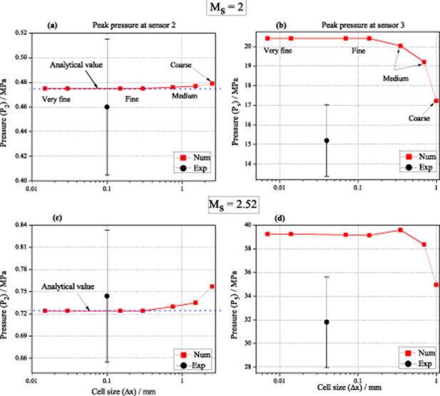
Figure 10. Results of mesh independency study compared with analytical (wherever possible) and experimental data. The subfigures are for peak pressure measurement at (a) sensor S2 for Ms = 2; (b) sensor S3 for Ms = 2; (c) sensor S2 for Ms = 2.52; (d) sensor S3 for Ms = 2.52.
Download figure:
Standard image High-resolution imageIn order to substantiate the validity the code, a numerical time of arrival study was performed for several Ms and compared with the corresponding experimental values. Since the acceleration inside the test section was continuous, the time of arrival was unique to each particular Ms and served as a base for the comparison study. The results of the test plotted in figure 11(a) shows good agreement between the experimental and numerical values. The scheme accurately predicts the time of arrival of the shock front for all tested Ms. Conversely, this establishes the fact that the convergence of the incident shock and divergence of the reflected shock was also accurately predicted by the simulation along with the development of its corresponding properties. First let us focus on the converging portion of the shock wave. The numerically estimated average velocity of the shock front in the converging test section is plotted in figure 11(b). The acceleration is relatively slower in the initial part of the convergence channel compared to the last quarter where it accelerates rapidly. Using this convergence method, the shock wave with an initial velocity of 806 m s−1 accelerates to velocity close to 2550 m s−1 for the current Ms.
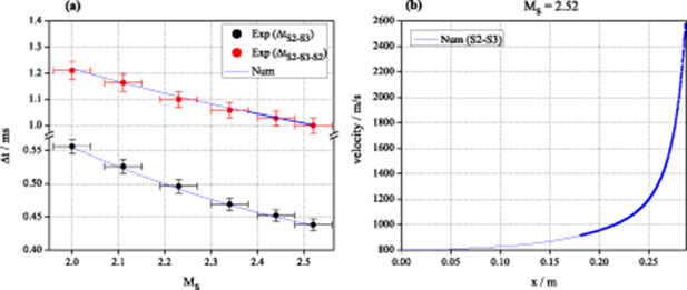
Figure 11. (a) Experimental and numerical time of arrival comparison for several Ms obtainable in the shock tube facility. (b) Numerical estimate of average velocity of the initial shock wave with Ms = 2.52 as it propagates through the test section from S2 to S3.
Download figure:
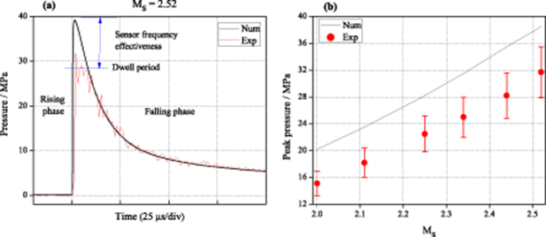
Standard image High-resolution imageThe comparison between both experimental and numerical pressure profiles at location S3 for one particular Ms = 2.52 is plotted in figure 12(a). Note that the simulation was started with similar initial conditions as with the experimental case and the resulting profile was juxtaposed with the sensor data. As verified by the time of arrival plot (figure 11) between S2 and S3, the trajectory and therefore the strength of the shock were accurately predicted by the simulation. This in turn confirms that S3 was impacted by a shock front of similar strength in both experiments and numerics. Despite that, the simulation predicts a relatively higher peak pressure compared to the experimental profile. On closer inspection, the differences arise only in the peak pressure estimation on the rising phase while both the profiles almost repeat each other and follow a similar trend otherwise.
Figure 12. Comparison between experimental and numerical, (a) pressure profile measured at S3 for Ms = 2.52 shock wave; and (b) peak pressures at S3 for various Ms (mean).
Download figure:
Standard image High-resolution image
As shown earlier in figure 11(b), the initial incident shock accelerates very quickly during its final quarter of propagation with its velocity reaching approximately 2550 m s−1 at the sensor S3. The reflection of such a strong shock wave is a very fast occurring event, and for the case plotted here, simulation predicts the time taken to reach the peak pressure of 39.2 MPa from atmospheric conditions to be approximately 1 µs. Upon impact, the sensor takes 1 µs to start recording during which the shock has travelled back a distance of ∼2 mm. Within this distance, the region becomes chaotic with the bombardment of consecutive expansion waves (generated by the divergence of the reflected shock wave) travelling towards the sensor face and reflecting back again. This process gradually reduces the pressure built-up by the incident shock wave. So by the time the sensor's element starts responding, the real pressure achieved is effectively lower. The sensor, with its 500 kHz stated resonant frequency, was still able to accurately measure almost 90% of the overall profile despite its 'unpreparedness' to respond to such ultra-fast dynamic processes occurring near the peak. During this period, the profile oscillates and hangs resulting in a 'dwell' period. Once the reflected shock wave propagates a certain distance, the reflected region is steadied and the profile declining effect was clearly picked up by the sensor following the dwell period during the falling phase. Since the numerical sensor had no such limitations, it was able to estimate the profile more accurately at the peak. The numerical profile can be seen as a reference that engulfs and completes the experimental profile. As shown in figure 12(b), this effect exists universally for all Ms tested in this study. Therefore the numerical profile can be used as a reference profile in order to establish the effectiveness of the sensor in terms of frequency response and pressure amplitude measurements. Ideally sensors with much shorter rise time and higher frequency response should be able to close this gap between the reference and the measured profile.
During the reflected shock wave propagation towards the sensor S2, a few other parameters like boundary layer interaction and shock geometry upon reflection needs to be addressed. Boundary layers are generally created at the wall when there is a flow with finite velocity. Since the incident shock wave was travelling into the gas at rest, there was no generation of boundary layer ahead of the shock path. Consequently boundary layers cannot affect the peak pressure generation. Also pressure across a boundary layer is constant which actually enables the use of pressure sensors in flow dominated regions. Despite the Reynolds number being very high in this work implying very high inertial forces relative to viscous forces, it could interact with the reflected shock thereby decelerating it. However, this potential deceleration should only affect on the falling phase profile as well as the time taken to reach S2 from S3. The numerical simulation solves for Euler equations making it unable to resolve boundary layer effects. However, comparing the falling phase profile traced by the simulation with the experimental result in figure 12(a), no distinct features are observed. Also the experimental time taken to travel from S3 to S2 matches with the simulation predicted time as shown in figure 11(a). This demonstrates that the effect of the boundary layer on the pressure generation should be negligible. Similar argument holds true for non-uniform reflection of the shock wave at the sensor face. Note that the simulation geometry was constructed with radial boundary at the end to ensure perfect reflection of the face. It is hard to show evidence on the structure of the reflected shock wave but on a quantitative basis it had no distinct effect on the resulting pressure profile despite its randomness.
The numerical peak pressure is sensitive to variations in incident Ms. As the value depends on the reliability of the experimental Ms calculation, it is advantageous to perform the simulation for each individual experimental run rather than for the mean value. By calculating Ms per run and subjecting the simulation based on it, the cumulative history of shock generation effects like losses in FOV and small deviations in  can be excluded. These losses would only impact the strength of the shock wave which would be measured for each case separately. This invariably reduces the uncertainty in Ms to 1.3% which translates to
  3.4% uncertainty in peak pressure determination through numerical simulation (table 3). Future works could be dedicated towards further reduction of this uncertainty.
Table 3. Effect of Ms uncertainty on numerical peak pressure value.
| 1.975 | 19.8 | 2.9% |
| 2 (actual) | 20.4 | 0% |
| 2.025 | 21.1 | 3.4% |
| 2.49 | 38.1 | 2.8% |
| 2.52 (actual) | 39.2 | 0% |
| 2.55 | 40.4 | 3.1% |
4. Conclusion
When calibrating a sensor measuring pressure dynamically, determining some important properties like sensitivity, amplitude, resonant frequency, rise time and overshoot, prove the effectiveness of the sensor for a particular application/situation. Although uniform cross-section shock tubes were efficient in determining said properties, their generated pressure amplitudes in the lower ranges limit its potential to be used as a standard across wider ranges. In this paper, we have addressed this issue by successfully demonstrating a technique of converging the incident shock wave that increases the amplitude to the medium-high range with a great potential to be extended into even higher amplitudes. A converging test section was constructed in a way that it smoothly varied in diameter from 80 mm to 7 mm through a transformation section (TS) and a conical section (CS). An initially plane shock wave of Ms = 2.52 underwent a transformation into spherical wave in the TS and upon further convergence in the CS reached almost thrice its initial Ms. Correspondingly, its peak pressure increased from 3 MPa (without the converging test section) to almost 40 MPa within 3.4% uncertainty (based on numerical reference profile), demonstrating the capability of the set-up for realizing high pressure amplitudes. Comparing the profile traced by the sensor that is unique to each Ms with the numerical reference profile provided a measure of the effectiveness of the sensor in terms of its sensitivity and frequency response. To this end, the current technique of transient pressure amplification extends the capacity of proven shock tube method in the realm of dynamic calibration.
Acknowledgments
The financial support by the European Metrology Programme for Innovation and Research (EMPIR) is gratefully acknowledged. This project has received funding from the EMPIR programme co-financed by the Participating States and from the European Union's Horizon 2020 research and innovation programme.