


Abstract
In this paper, we introduce a robust method for dynamic characterization of pressure measuring systems used in time-varying pressure applications. The dynamic response of the pressure measuring systems in terms of sensitivity and phase as a function of frequency at various amplitudes of the measurand can be provided. The shock tube which is the candidate primary standard for dynamic pressure calibration at the National Laboratory for pressure, Sweden, was used to realize the dynamic pressure. The shock tube setup used in this study can realize reference pressure with amplitudes up to 1.7 MPa in the frequency range from below a kilohertz up to a megahertz. The amplitude of the realized step pressure was calculated using the Rankine–Hugoniot step relations. In addition, the accurate time of arrival of the generated shock at the device under test (DUT) was measured using an optical probe based on shadowgraphy. The optical detector has a response time in nanosecond time scale which is several orders of magnitude faster than the response time of any pressure measuring system. Hereby, the latency between physical stimuli and response of the DUT can be measured. By the knowledge of the amplitude and the accurate time of arrival of the reference step pressure, the transfer function of the DUT can be calculated and presented in Bode diagrams of sensitivity and phase response versus frequency. The uncertainty in sensitivity and phase measurements was estimated. The information provided by this work is useful for developing reliable models of dynamic pressure measuring system and provide accurate information about their dynamic response. That in turn will contribute to establish a traceability chain for dynamic pressure calibration.
Export citation and abstract BibTeX RIS

Original content from this work may be used under the terms of the Creative Commons Attribution 4.0 licence. Any further distribution of this work must maintain attribution to the author(s) and the title of the work, journal citation and DOI.
1. Introduction
Accurate measurement of time-varying pressure is of great importance in many applications such as turbomachinery, automotive industry, and human health [1–4]. To obtain accuracy in dynamic measurements, contributions to the signal from the sensor must be separated from the measurand. For dynamic measurements such compensation must also consider time. Models for compensation should be rooted in the physical behaviour of the sensors.
A common way to measure dynamic pressure is to measure the displacement or deformation of a mechanical element due to the force imposed by the pressure. A general and simple model to describe such a mechanical system is by a linear second-order differential equation [5, 6],  . Here f(t) is the external force generated by the acting pressure, m is the mass of the moving object, c indicates the damping leading to energy dissipation and k is the spring constant that restores the system. The first term in the left-hand side of the equation represents the inertia of the system, the second term is the system damping, and the third term indicates the restoring force. By applying a Laplace-transform to the differential equation, the response of the system to the external force may be described in frequency space. When the acting force, in our case pressure, varies with a frequency lower than the natural frequency of the system, the restoring force dominates the other two terms, and the phase difference between the acting pressure and the system response is small (approximately zero). If the acting pressure has the same frequency as the natural frequency of the system, the restoring and inertial terms cancel each other resulting in π/2 phase difference between the acting pressure and system response. That in turn causes the system to end up in a resonant mode in the case of underdamped oscillations. In the case where the acting pressure has frequency exceeds the natural frequency, the inertial term starts to dominate, resulting in a phase lag of π.
The model above illustrates the basic effects that are expected from a dynamic pressure system. However, many real features are not considered by it. Coupled movements between the sensing element and other components, may they be sensor internal or external fittings, are not included [7, 8]. Neither is any time delay between the event of input pressure and the corresponding system response due to latency in the signal process. External electrical equipment, like charge amplifiers, may be characterized separately by electrical means but this is not possible for the pressure sensing component. Robust calibration is essential to quantify the real behaviour of a dynamic sensing system.
Dynamic calibration should provide information about both sensitivity and phase response of the measuring system as a function of frequency at various amplitudes of the measurand. In the stricter sense of the term 'calibration', meaning accredited or acknowledged by the CIPM mutual recognition arrangement, dynamic calibration is currently lacking [9]. Several National Metrology Institutes are working to establish a traceability chain of time-varying pressure measurements [10–15]. To establish the traceability, developing the candidate primary standards that can realize time-varying pressure with a specific frequency bandwidth and amplitude is important [16, 17]. In addition, developing robust methods for calculating the dynamic response of time-varying pressure measurement systems is needed [18, 19].
Due to lack of traceable dynamic calibration, dynamic pressure measuring systems are presently calibrated using quasi-static methods reporting sensitivity only with respect to pressure. Quasi-static approaches assume that the pressure measuring system respond in the same way for time-varying pressures as for static pressures resulting in large uncertainties in the measurements of time-varying pressures for the end users. The sensitivity of a pressure measuring system may vary with the frequency of the applied pressure resulting in an error in the measured amplitude. In addition, a time delay (latency) between the pressure stimuli and output signal can cause errors in the time domain of dynamic pressure measurements.
Shock tubes are available candidates to realize high-frequency reference pressures. In contrast to other candidates for dynamic pressure primary standards, such as drop-weight devices [20, 21] and piston-in-cylinder pressure generators [22, 23], shock tubes can realize reference step pressure with risetime well below 1 μs, thus exciting frequencies in the megahertz range. The lower frequency limit is proportional to the reciprocal of the time during which the realized step pressure remains constant. By knowing the amplitude and the accurate time of arrival of the realized reference step pressure at the device under test (DUT), the transfer function of the DUT can be calculated and presented in Bode diagrams of sensitivity and phase response versus frequency.
The amplitude of the reference step pressure can be determined by the simplified Rankine–Hugoniot step relations [24]. To apply Rankine–Hugoniot step relations, the speed of the shock front is needed. That can be determined using trigger systems mounted at known positions along the shock tube. These trigger systems can also be used to determine the time of arrival of the shock front at the DUT, however, this requires that their respective latency is known. For available pressure measuring systems, traceable latency is lacking. In effect, the measured time of arrival of the shock front at DUT is a relative time with respect to the response of the trigger systems and not to the actual pressure stimuli.
To measure the absolute response time of the DUT with respect to pressure stimuli, we equipped our shock tube with a specially devised optical probe. The response time of the optical probe is on the nanosecond time scale, which is several orders of magnitude faster than the response time of the pressure measuring systems. Hereby, the time of arrival of the shock front at the DUT can be accurately detected independently of the response time of any pressure measuring systems. The used optical probe is based on shadowgraphy which is a well stablished non-invasive optical technique used to study transient processes and has been used for imaging and diagnosing shock waves generated in different applications [25, 26].
To demonstrate the applicability of the full dynamic characterization method, four different pressure measuring systems in terms of their working mechanism (piezoelectric, piezoresistive), measuring range (pressure amplitude, frequency, temperature, etc...) and amplification method (internal or external) were tested. The transfer function for each system was calculated and presented in Bode diagrams of sensitivity and phase response versus frequency.
2. Experimental setup and procedure
In the following, the experimental setup used to realize the reference step pressure as well as the latency measurement setup will be introduced. In addition, a description of the selected devices under study and the conditions they were characterized at will be presented.
2.1. Dynamic pressure realization
Figure 1 shows a schematic illustration of the shock tube used to realize dynamic pressure steps. The shock tube consists of two parts; the driven section, filled with low-pressure driven gas, and the driver section that contains a high-pressure driver gas. The driven and driver sections have an inner diameter of 100 mm and lengths of 7 m and 3 m, respectively. The two sections are separated by a fast-opening valve (KB-80-20, ISTA Pneumatics). The driven section is equipped with six piezoelectric pressure sensors (113A21, PCB) mounted at well-defined positions on the circumference along a straight line parallel to the central axis of the shock tube. These sensors are used to measure the propagation speed of the generated shock waves.

Figure 1. Schematic illustration of the shock tube, FOV: fast-opening valve, M: mirror, DUT: device under test.
Download figure:
Standard image High-resolution imageStatic absolute pressure transmitters were mounted on the driver section (EJX 310A, Yokogawa) and the driven section (EJX 510A, Yokogawa) to monitor the initial pressures of these volumes. The driver and driven sections can be filled, vented, and evacuated independently. To ensure pure and well-known gas composition in driven and driver sections, the system was equipped with a dry roots vacuum pump (NeoDry 15E, Kashiyama) for evacuation of the volumes before filling with appropriate gases. In these experiments, Ar (99.999%, Air Liquide) and CO2/N2 mixture with a molar ratio of 30/70% ± 0.30% of 99.998% CO2 and 99.999% N2 (Air Liquide) were used in the driven section. While in the driver section, N2 and He (99.999%, Air Liquide) were used.
The shock tube was positioned in a temperature-controlled laboratory. The initial gas temperature was measured using a calibrated temperature measuring system consisting of four thermocouples (type k) spot welded at different positions along the circumference of the shock tube. The thermocouples were connected to a universal input module (Fluke 2638A-100) which was in turn coupled to digital multimeter (Fluke 2638A). A Pt100 temperature sensor was connected to the same module and placed among the external bundled cold junctions of all thermocouples. The readings of the thermocouples were taken after reaching pressure stability. As our system is leak tight and is hermetically isolated this in turn is an indication of temperature stability. This process takes approximately 10 min to 15 min.
2.2. Latency measurement
For latency measurement, the shock tube was equipped with an optical probe. An extra section with the same inner diameter as the shock tube (100 mm) and a length of 100.8 mm with an optical access was connected to the shock tube. A He–Ne laser (632.8 nm wavelength, 0.8 mm beam diameter and 5.0 mW output power) was used as a light source. The laser beam was guided to a photodetector (Thorlabs, PDA10A2) after passing through the shock tube, perpendicular to shock propagation direction thus being parallel to the plane of the shock front. The photodetector model is rated with a response time around 2.3 ns and response wavelength in the range of (200–1100) nm. The distance between the laser beam and the end-wall plate of the driven section was measured using a calibrated depth micrometer (Mitutoyo) with a resolution of 0.01 mm.
2.3. Devices under test and experimental settings
Four dynamic pressure measuring systems were dynamically characterized:
- PCB 113A21 piezoelectric sensor with a PCB 483C Series signal conditioner, (system #1).
- AVL GU24D piezoelectric sensor with a Kistler 5064C charge amplifier, (system #2).
- Keller M8coolHB piezoresistive sensor head and measurement amplifier, (system #3).
- Kistler 4049A piezoresistive sensor with a Kistler 4622A amplifier, (system #4).
The respective DUT was flush mounted at the centre of the end-wall plate of the driven section in all experiments. The output signal from the respective DUT, the optical probe and the side-wall sensors were acquired using an eight channel 12 bit 60 MS s−1 per channel oscilloscope (PXI-5105, NI) with a maximum sampling size of 106 samples. In this study, we used the maximum sampling size and optimized the sampling rate according to the DUT properties. LabVIEW software was used for data acquisition. The experimental and data acquisition settings for different DUTs are listed in table 1. The difference in settings reflects the nominal properties of the respective DUT.
Table 1. A list of the experimental and data acquisition settings for different DUTs.
| DUT | Driven gas | Driver gas | Nominal step pressure/kPa | Sampling rate/MS s−1 |
|---|---|---|---|---|
| System #1 | Ar | He | 800 | 60 |
| System #2 | Ar | He | 800 | 60 |
| System #3 | CO2/N2 | N2 | 500 | 20 |
| System #4 | CO2/N2 | N2 | 500 | 20 |
In all experiments, the driven gas pressure was kept at 100 kPa.
3. Analysis
The procedures of evaluating the reference step pressure in terms of amplitude and time of arrival at the DUT will be presented. The amplitude of the reference pressure was calculated using the Rankine–Hugoniot step relations and the time was measured using the optical probe. In the frequency domain, the dynamic response of the DUT in terms of sensitivity and phase will be introduced. The method of estimating the uncertainty budget for sensitivity and phase calculation, respectively, will be introduced.
3.1. Time domain
3.1.1. Pressure amplitude calculation
The realized reference step pressure at the end-wall plate of the driven section is assumed to have the shape of a Heaviside step function. A typical realized step pressure recorded by a DUT flush mounted at the centre of the end-wall plate and the four side-wall sensors closest to the end-wall plate is shown in figure 2. The amplitude of the step pressure is determined by the simplified Rankine–Hugoniot relations with the knowledge of the Mach number of the incoming shock front M and the initial static pressure of the driven gas p1 [24].

Figure 2. A typical recorded step pressure realized by the shock tube at a nominal pressure 800 kPa. The optical signal is also shown in the figure.
Download figure:
Standard image High-resolution imageThe Mach number of the incoming shock front is the ratio of its propagation speed in the laboratory frame v and the speed of sound in the undisturbed driven gas a1:

v is determined by fitting a quadratic polynomial to the time of arrival of the shock front at the positions of the four side-wall sensors closest to the end-wall plate (see figure 2). The time of arrival of shock front at the positions of the side-wall sensors was determined by using the cross correlation between their respective signal and a truncated (200 samples) signum function. This gives the relative time of arrival of the shock front at the positions of the side-wall sensors. Due to the unknown latency of these systems, this data can only be used to calculate the speed of the shock front, not to provide any fixed reference time. The derivative of position with respect to time at the end-wall plate position represents the shock propagation speed. A quadratic function was chosen to account for the deceleration of the shock front due to energy losses. With the quadratic fit of position versus time, the speed of the shock front was assumed to be linearly decreasing with time. The linear behaviour of the speed with time is the simplest approximation of a non-constant speed. The use of quadratic fitting was validated, and it will be described in detail in the next section.
The speed of sound in the undisturbed driven gas a1 was calculated using the initial parameters of the driven gas; specific heat ratio γ1, molecular mass m1, its measured initial absolute temperature T1 and the gas constant R as following:

From the calculated Mach number M and the initial static pressure of the driven gas, p1 the pressure behind the incoming shock front p2 is given by:

The pressure behind the reflected shock front at the end-wall plate p5 can be calculated as:

The amplitude of the reference step pressure p is calculated as the difference between the pressure behind the reflected shock front p5 and the initial pressure of the driven section p1:

3.1.2. Latency calculation
From the distance between the DUT and the side-wall sensors, the relative time response of the DUT with respect to the side-wall measuring systems can be calculated. The delay in response time of these side-wall measuring systems is unknown. However, to estimate the absolute time response of the DUT, i.e. in relation to the interaction with the shock front, the shock tube was equipped with the optical probe described in section 2.2. The laser beam is guided to the photodetector after passing through the shock tube. When the shock front interacts with the laser beam, the pressure gradient refracts the laser beam, and a significant decrease of the beam intensity is detected by the photodetector. The optical detector has a response time in nanosecond time scale which is several orders of magnitude faster compared to the response of the pressure measuring systems. Therefore, it can be used as a reference to detect the time of shock front impingement on the DUT. Figure 3 shows a typical recorded step pressure, the corresponding calculated reference step pressure, and the recorded optical signal. To calculate the latency of the DUT the following procedures were applied:
- The distance between the laser beam edge closest to the incoming shock front and the end-wall plate of the driven section where the DUT was flush mounted was measured using a depth micrometer. The optical signal was monitored, and the edge of the laser beam located where the signal was completely blocked by the micrometer.
- Fitting a quadratic polynomial to the time of arrival of the shock front at the positions of the four side-wall sensors closest to the end-wall plate. The validity of this fitting was checked by flush mounting a sensor to the end-wall plate. This sensor was of the same model as the side-wall sensors and was connected to the same signal conditioner and to a parallel channel to the data acquisition system. A quadratic fit with respect to time representing the time–position relation measured by the side-wall sensors (1–6) was applied. The deviation in time of arrival of the extrapolated quadratic fit at the end-wall plate and the recorded time of arrival by the end-wall sensor was checked. Five shots were recorded, the mean value of the deviation was negligible. The variance width between shots was considered in the uncertainty calculation.
- From the quadratic fit, the time of arrival of the shock front at the respective positions of the laser beam edge and the end-wall plate can be estimated by extrapolation. The relative time between them (Δt) is calculated.
- The time at which the shock front interacts with the laser beam edge closest to the incoming shock (toptic) is determined from the recorded optical signal (see figure 3).
- The absolute time of the shock front arriving at the DUT (tref), in the time frame of the data acquisition device, is calculated as toptic + Δt.
- The latency of the DUT is then calculated as the difference between the recorded time response of the DUT (trec) and tref, (see figure 3).

Figure 3. A typical recorded step pressure, the corresponding calculated reference step pressure and the recorded optical signal.
Download figure:
Standard image High-resolution image3.2. Frequency domain
For calculating the sensitivity and phase response of the DUT versus frequency, the following procedures were applied:
- Fast Fourier transform (FFT) was applied to both the recorded signal from the DUT and the corresponding reference step pressure (ideal Heaviside step function with amplitude calculated according to equations (1)–(5) and located at the calculated tref) using a Gaussian window centred at pressure discontinuity of the recorded step pressure.
- The ratio between the average of FFT of five recorded signals and the average of FFT of the corresponding reference step pressures was calculated.
- The frequency-dependent sensitivity was obtained by taking the magnitude of the calculated ratio.
- The frequency-dependent phase was obtained by taking the angle of the calculated ratio.
In case of studying system #1 and system #2, the full width at half maximum (FWHM) of the Gaussian window was 1 ms. While the window has a FWHM of 1.6 ms and 6.5 ms when characterizing system #3 and system #4, respectively.
3.3. Uncertainty budget
3.3.1. Uncertainty in sensitivity calculation
The amplitude of the reference step pressure is depending on a set of input parameters listed in table 2 along with their respective standard uncertainty. In the case when the input parameter is a measurand the respective measuring device is calibrated. To assess the influence of each source on the uncertainty on p5, we employed a previously developed Monte Carlo method [27]. In the Monte Carlo method, p5 is calculated according to relations described above 106 times with the input parameters independently and randomly distributed according to table 2. The standard deviation of the resulting distribution of p5 is the standard uncertainty in p5 ( ).
).
Table 2. List of the input parameters in the step pressure calculation and their corresponding standard uncertainty.
| Parameter | Standard uncertainty, k = 1 | Distribution |
|---|---|---|
| Temperature (K) | 0.7 | Rectangular |
| Time (s) | 0.5 × 10⁻⁶ | Normal |
| Side-wall sensors positions (m) | 10–4 | Normal |
| Specific heat ratio γ1 | 10–4 | Normal |
| Initial driven pressure p1 (Pa) | 360 | Normal |
- The uncertainty in temperature considers the uncertainty in calibration of the temperature measuring system described in section 2.1, and the variance between the four thermocouples readings along the shock tube.
- The uncertainty in time comprises the time resolution of the measurements (sampling rate of 60 MHz and 20 MHz were used in this study) and the deviation between the recorded and the fitted arrival time of the shock front at the side-wall sensors positions.
- The side-wall sensors positions were measured and the uncertainty of the measurement was used.
- The value of the dimensionless specific heat ratio γ1 of different driven gases used in this study was taken from literature [28] with absolute uncertainty of 10–4.
- The uncertainty in p1 was calculated considering the following parameters; temperature effect, drift effect, the uncertainty in the calibration of the pressure transmitter including the signal conditioner at different pressure levels.
The standard uncertainty in step pressure amplitude (up ) was calculated according to:

Since the uncertainty in p5 is dominated by the uncertainty in temperature is thereby assumed to be uncorrelated with p1.
The corresponding standard uncertainty in sensitivity ( ) was calculated as:

where Vsig is the amplitude of the recorded signal. In the final uncertainty in sensitivity, repeatability was also considered. Five shots were recorded at each nominal pressure level and the standard uncertainty in sensitivity at each frequency due to repeatability ( ) was calculated as:

The total standard uncertainty (k = 1) in sensitivity  was estimated as:

The expanded uncertainty (k = 2) in sensitivity (US) was calculated as:

3.3.2. Uncertainty in phase calculation
A list of the parameters that contribute to the uncertainty in calculating the absolute time response of the DUT (tref) and their corresponding standard uncertainty is shown in table 3.
Table 3. List of the input parameters in tref calculation and their corresponding standard uncertainty.
| Parameter | Standard uncertainty, k = 1 | Distribution |
|---|---|---|
| Time of arrival of the shock front at the optical probe, toptic (s) | 0.1 × 10⁻⁶ | Normal |
| Distance between laser beam edge and the end-wall plate, x (m) | 0.1 × 10⁻³ | Normal |
| Speed from the extrapolation using the quadratic fit (relative contribution) (%) | 0.18 | Rectangular |
- The uncertainty in reading toptic (
 ) from the recorded optical signal was estimated to be 0.1 μs.
 - The uncertainty in the relative time of arrival of the shock front at the respective positions of the laser beam edge and the end-wall plate (Δt) stems from the uncertainty in their mutual distance and the uncertainty in the shock front speed from the validation of the quadratic fit. Only the first order terms in uncertainty in speed were considered.
- The uncertainty in distance (ux ) was taken to be 0.1 mm. Both uncertainty from the calibration of the used depth micrometer (2.5 μm) and the repeatability in measurements were considered.
- The shock front speed contribution to the uncertainty was taken as a relative uncertainty in Δt of 0.18% obtained from the validation of the quadratic fit.

The standard uncertainty in Δt (uΔt ) was estimated as:

The standard uncertainty in tref ( ) was then calculated:

The corresponding standard uncertainty in phase ( ) at each frequency (f) was given by:

The uncertainty in phase due to repeatability was also considered. Five shots were recorded at each nominal pressure level and the standard uncertainty in phase at each frequency due to repeatability ( ) was calculated as:

The total standard uncertainty (k = 1) in phase  was calculated as:

The expanded uncertainty (k = 2) in phase (Uφ ) was:

4. Results and discussion
To demonstrate the applicability of the method to describe the properties of dynamic pressure measuring systems, we have investigated four setups comprising measurement equipment from different manufacturers. The results should not be interpreted as a comparison between the measurement equipment as we have neither regarded the targeted measurement application of the respective equipment nor the usage history of the components. The equipment presented here were selected because they exhibit qualitatively different characteristics and were readily available at our laboratory.
The shock tube setup used in this study can realize dynamic pressure with amplitude up to 1.7 MPa and frequency content above 500 kHz. Since this paper focuses on establishing the method for calculating the dynamic response of the DUT, we present the results of each DUT at a single pressure level. The respective levels were selected with regards to the measurement range of the sensor and available step pressures from the shock tube. The sensitivity and phase response of each DUT were calculated according to the procedure described in section 3.
Figures 4–7 show the results from different systems tested in this study. The figures show the recorded step pressure in time domain (single shot) and the corresponding calculated sensitivity (average of five shots) and phase (average of five shots) response in frequency domain for each system, respectively. In all figures the frequency dependent uncertainty (95% coverage probability) is shown. In the figures, the uncertainties are expressed continuously in the full frequency range, while in the text we present tabulated values at selected frequencies.

Figure 4. (a) A recorded step pressure (single shot) using system #1 at nominal pressure of 800 kPa, (b) and (c) the corresponding calculated sensitivity and phase, respectively, (average of five shots each) as a function of frequency. The blue lines in (b) and (c) represent the expanded uncertainty (k = 2) in sensitivity and phase, respectively.
Download figure:
Standard image High-resolution imageFrom the recorded signal in time domain, information about the risetime (the time required for the output signal to rise from 10% to 90% of its final value) and the percentage overshoot of the DUT can be obtained. However, we argue that the DUT characteristics are best described in the frequency domain.
In the amplitude, or more specific the sensitivity, part of the frequency responses attention should be paid to the region close to 0 Hz and to regions with peaks or valleys. The sensitivity approaching 0 Hz corresponds to the quasi-static sensitivity. The region above 0 Hz in which the sensitivity remains constant is the region where a quasi-static calibration of sensitivity is valid for the specific system. The width of this region may be regarded as the bandwidth of the system. As seen from the results, the two piezoelectric systems have much higher bandwidth than the piezoresistive systems. N.B., our method has a limited resolution in frequency and thus does not represent the drop in sensitivity of piezoelectric systems in the very lowest frequency regimes.
For overdamped systems, the sensitivity eventually drops above some cut-off frequency. The cut-off frequency limits the risetime in the temporal space but the drop in sensitivity results in little 'ringing' after transient events, cf figure 7 If the sensitivity instead transits into a peak in frequency space, the response in the time domain is accompanied by an overshoot and pronounced ringing after transient events (underdamped sensors), this is clearly seen in figure 6.
The origin of peaks can be either resonant behaviour in the sensing element or vibrational modes in the system or the mounting. Hints of the origin of a specific peak can be found in the phase part of the response function.
The phase part of the frequency response presents the delay of the system response with respect to stimuli as the argument of a sinusoidal function with a given frequency. In effect this means that a constant delay is evident as a linear slope of the phase response in the whole frequency range. This is clearly seen in figures 6 and 7. A pure resonance, as seen in figure 5 at 96 kHz, will have a local cumulative drop of π radians. Interference from coupled vibrations have other characteristics. In short, a drop of π radians is a good fingerprint of resonances, or the natural frequency, of the sensing element and a constant slope is a fingerprint of a fixed delay in the signal.
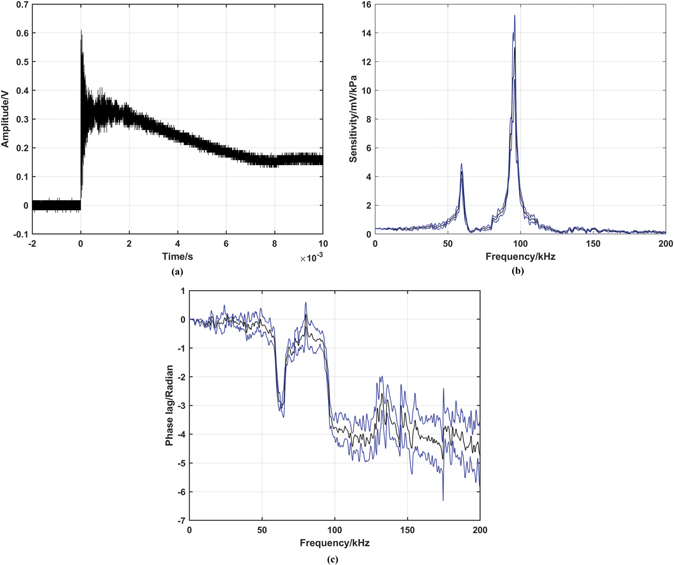
Figure 5. (a) A recorded step pressure (single shot) using system #2 at nominal pressure of 800 kPa, (b) and (c) the corresponding calculated sensitivity and phase, respectively, (average of five shots each) as a function of frequency. The blue lines in (b) and (c) represent the expanded uncertainty (k = 2) in sensitivity and phase, respectively.
Download figure:
Standard image High-resolution imageDetailed results of each tested system will be presented and discussed in the next sections.
4.1. Piezoelectric pressure measuring systems (system #1 and system #2)
A recorded step pressure at a nominal pressure of 800 kPa is shown in figures 4(a) and 5(a) for system #1 and #2, respectively. The corresponding calculated sensitivity and phase response of system #1 are shown in figures 4(b) and (c), respectively. While figures 5(b) and (c) show the calculated sensitivity and phase response, respectively for system #2.
For the two tested piezoelectric pressure measuring system (system #1 and #2), figures 4(a) and 5(a), showing the respective system response in the time domain, indicate that the step pressure has constant amplitude for short time about 1.5 ms for system #1 and 2 ms for system #2. In these experiments He was used as a driver gas which results in faster expansion wave and short plateau. The short plateau was compensated by a narrower window during FFT. The durations of the plateaus are thereby long enough to permit the assumption of a Heaviside step inside the Gaussian windows. Both systems have a rapid risetime but a percentage overshoot of 14% can be seen for system #1 while system #2 has 72%. Figure 5(a) shows that the signal level from system #2 is low but we believe that this has no consequences to the purpose of this paper. Figures 4(b) and 5(b) show the sensitivity as a function of frequency of the two systems, respectively. The average sensitivity of five shots is presented for each system. System #1 has a constant sensitivity which is on average about 3.36 mV kPa−1 up to 50 kHz. Figure 5(b) shows that system #2 has a constant response of about 0.40 mV kPa−1 up to 30 kHz. A resonance is present at 96 kHz for system #2 which relates to the overshoot in the time domain.
Both systems have peaks in the amplitude response that do not have the typical resonant behaviour in the phase response. These features can be seen from 150 kHz to 300 kHz for system #1 and around 60 kHz for system #2. We hypothesize that these peaks originate from mechanical vibrations that affects the system-pressure media coupling. Such vibrations could be system internal or occur in the mounting material. We believe that these features are possible to model and pose interesting future work.
The corresponding phase of both systems are presented in figures 4(c) and 5(c), respectively. The calculated average latency of system #1 is about 0.1 μs. This may be compared to the expanded uncertainty (k = 2) in time of arrival of the shock front at the DUT which is 0.54 μs. The fast response time results in phase lag close to zero up to 270 kHz. There is a phase jump of 2π radians around 310 kHz that may result from unresolved noise from vibration. For system #2, the calculated average latency is about 2 μs. The resulting phase lag can be seen in figure 5(c). The phase lag is gradually increasing with frequency reaching about −1 rad at 90 kHz and an expected phase lag of −π radians is seen around the resonance frequency 96 kHz. Phase lag corresponding to the hypothesized vibration peak at 60 kHz is obviously seen in the figure.
The expanded uncertainty (k = 2) in sensitivity calculation estimated using equations (6)–(10) is shown in figures 4(b) and 5(b) for system #1 and #2, respectively. The estimated expanded uncertainty in sensitivity for system #1 increases from about 0.14 mV kPa−1 (4.2%) close to 0 Hz to about 0.38 mV kPa−1 (11.3%) at 10 kHz. For system #2, the expanded uncertainty is about 0.02 mV kPa−1 (5%) close to 0 Hz and it is 0.03 mV kPa−1 (7.5%) at 10 kHz.
The expanded uncertainty in phase calculation estimated using equations (11)–(16) is shown in figures 4(c) and 5(c) for system #1 and #2, respectively. For system #1, the uncertainty increases from 1 mrad close to 0 Hz to about 110 mrad at 10 kHz. The significant increase in uncertainty at 310 kHz is from poor repeatability between shots at this frequency caused by unresolved noise as described above. For system #2, the uncertainty is about 6 mrad in the vicinity of 0 Hz and is about 70 mrad at 10 kHz.
4.2. Piezoresistive pressure measuring systems (system #3 and system #4)
Two piezoresistive pressure measuring systems were investigated. Figures 6(a) and 7(a) show a step pressure at a nominal pressure of 500 kPa recorded by system #3 and #4, respectively. The corresponding calculated sensitivity and phase in frequency domain of system #3 are shown in figures 6(b) and (c), respectively. While figures 7(b) and (c) show the calculated responses of system #4. For detailed information about sensitivity response of each sensor, insets showing the sensitivity up to 10 kHz are added to figures 6(b) and 7(b), respectively.

Figure 6. (a) A recorded step pressure (single shot) using system #3 at nominal pressure of 500 kPa, (b) and (c) the corresponding calculated sensitivity and phase, respectively, (average of five shots each) as a function of frequency. The blue lines in (b) and (c) represent the expanded uncertainty (k = 2) in sensitivity and phase, respectively. The inset in (b) is the zoomed in data up to 10 kHz.
Download figure:
Standard image High-resolution image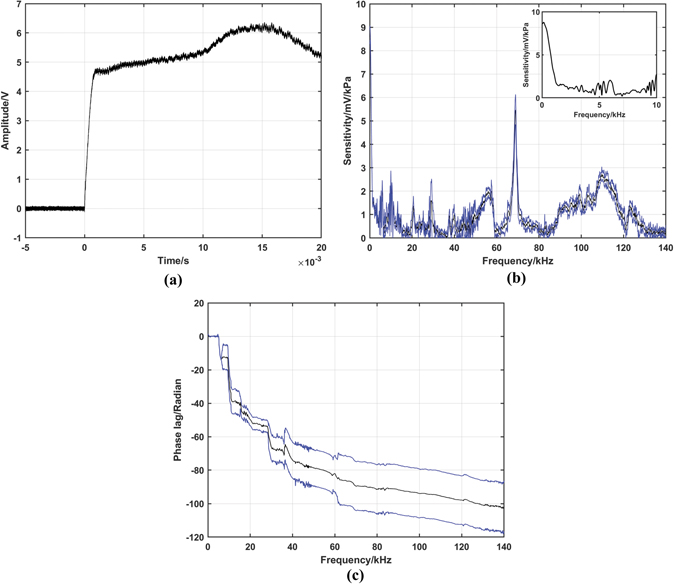
Figure 7. (a) A recorded step pressure (single shot) using system #4 at nominal pressure of 500 kPa, (b) and (c) the corresponding calculated sensitivity and phase, respectively, (average of five shots each) as a function of frequency. The blue lines in (b) and (c) represent the expanded uncertainty (k = 2) in sensitivity and phase, respectively. The inset in (b) is the zoomed in data up to 10 kHz.
Download figure:
Standard image High-resolution image
Figures 6(a) and 7(a) show that the step pressure remains with a longer plateau for sensors #3 and #4, respectively. In these experiments N2 was used as a driver gas which is a heavy gas that slows down the expansion wave. As a result, the reflected wave maintains constant amplitude longer time (compared to using light gases (i.e., He)) before it interacts with the expansion wave.
The underdamped system #3 has a rapid risetime of 2.6 μs with a percentage overshoot of about 147% and subsequent ringing. Figure 6(b) shows that the sensitivity of the sensor is about 3.27 mV kPa−1 around 0 Hz and increases with frequency to reach 6.84 mV kPa−1 at 10 kHz, which correlates to the undamped behaviour. The average latency of the sensor is about 14 μs. The corresponding phase lag is seen in figure 6(c). The phase lag gradually increases from zero to about −21 rad at 140 kHz. Some phase jumps of 2π radians due to noise can be seen in the figure.
System #4 is overdamped with a slow risetime of 626 μs but very little overshoot and ringing. Figure 7(b) shows that the sensor has a sensitivity of about 8.66 mV kPa−1 at 0 Hz and it steeply decreases to 1.42 mV kPa−1 at 1.5 kHz. A resonance is suggested at 69 kHz. The calculated latency of the sensor is 19.4 μs. The long-time lag due to latency produces phase lag that gradually increased with frequency to reach about −100 rad at 140 kHz, see figure 7(c). This phase lag is also including several 2π radians phase jumps due to unresolved noise.
The expanded uncertainty (k = 2) in sensitivity shown in figures 6(b) and 7(b) for system #3 and #4, respectively. The estimated expanded uncertainty for system #3 increases from about 0.12 mV kPa−1 close to 0 Hz to about 0.29 mV kPa−1 at 10 kHz. For system #4, the expanded uncertainty is about 0.30 mV kPa−1 close to 0 Hz and is 0.16 mV kPa−1 at 10 kHz.
The expanded uncertainty in phase calculation is shown in figures 6(c) and 7(c) for system #3 and #4, respectively. For system #3, it increases from 15 mrad close to 0 Hz to about 40 mrad at 10 kHz. For system #4, the uncertainty is about 0.06 rad in vicinity of 0 Hz and is about 7.25 rad at 10 kHz. This increase in uncertainty in phase for system #4 resulted from the unresolved noise.
5. Conclusion
In this paper, a robust method for dynamic characterization of time-varying pressure sensors was established. A shock tube was used to realize the time-varying reference pressure signal. The amplitude of the reference step pressure was calculated using the Rankine–Hugoniot step relations and the accurate time of arrival of the reference step pressure at the DUT was measured using an optical probe based on shadowgraphy. Our method primarily adds traceability to the measurements of the DUT latency. In hindsight we can conclude that the sensors we use to measure the speed of the shock front (the same model as system #1) are fast enough to assess the time of arrival of the shock front at the end-wall plate of the driven section with almost identical accuracy as we present here with our optical method, even without correcting their signals for latency. This was however impossible to tell prior to this study. By the knowledge of the amplitude and the time of arrival of the reference step pressure at the DUT, the transfer function of the DUT was calculated and presented in Bode diagrams of sensitivity and phase response versus frequency. In addition to the information about the lag between the incoming and outcoming signal from the DUT, the phase response provides also additional insights into the amplitude response of a sensor that allows to distinguish qualitatively between different types of features. The results show that the dynamic behaviour of each sensor is unique and differs from its static response. Therefore, characterizing dynamic pressure sensors under dynamic conditions is mandatory to obtain accurate measurements. Further investigation of the sources of vibrational signals and possible methods to mitigate this effect will be addressed in the incoming work.
Acknowledgments
The financial support by the Swedish Governmental Agency for Innovation Systems VINNOVA, grant number 2020-04320, is gratefully acknowledged.