

Abstract
We develop a relativistic treatment of interference between light reflected from a falling cube retroreflector in the vertical arm of an interferometer, and light in a reference beam in the horizontal arm. Coordinates that are nearly Minkowskian, attached to the falling cube, are used to describe the propagation of light within the cube. Relativistic effects such as the dependence of the coordinate speed of light on gravitational potential, propagation of light along null geodesics, relativity of simultaneity, and Lorentz contraction of the moving cube, are accounted for. The calculation is carried to first order in the gradient of the acceleration of gravity. Analysis of data from a falling cube gravimeter shows that the propagation time of light within the cube itself causes a significant reduction in the value of the acceleration of gravity obtained from measurements, compared to assuming reflection occurs at the face. An expression for the correction to g is derived and found to agree with experiment. Depending on the instrument, the correction can be several microgals, comparable to commonly applied corrections such as those due to polar motion and earth tides. The controversial 'speed of light' correction is discussed.
Export citation and abstract BibTeX RIS

Original content from this work may be used under the terms of the Creative Commons Attribution 3.0 licence. Any further distribution of this work must maintain attribution to the author(s) and the title of the work, journal citation and DOI.
1. Introduction
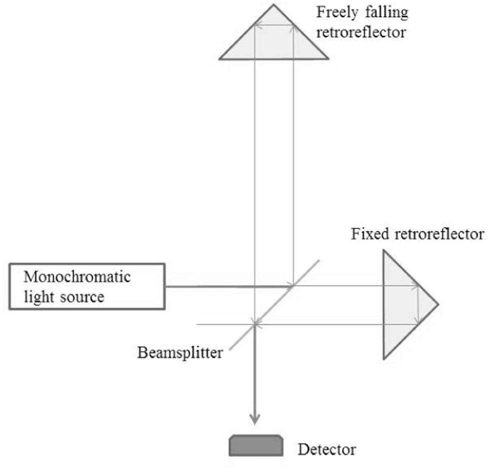
In a typical falling cube gravimeter, whose purpose is to measure the acceleration of gravity g with precision, a reference beam passes through a beam splitter where part of the beam is sent vertically to a falling corner cube reflector in an evacuated chamber. The cube is accelerated by gravity so the reflected beam suffers first- and second-order Doppler shifts as well as other effects; upon mixing with the reference beam back at the beamsplitter a beat frequency is generated having a rapidly increasing frequency chirp. In the gravimeter analyzed in this paper, a time stamp is recorded repeatedly after some fixed increment in the number of zero crossings of the beat signal. The time series depends on the strength g of the acceleration of gravity and on its gradient, on the structure of the retroreflector, and the position and velocity of the cube at the initial instant of release; the initial position and velocity and g are then extracted from the data. Typically a great many drops are averaged to obtain the value of g; fractional uncertainties of the order of  are currently obtained after applying several corrections that are of microgal order;
  .
.
A freely falling, locally inertial system can provide an application of the Principle of Equivalence: after expanding the gravitational potential in a Taylor series about the origin of local freely-falling coordinates and transforming the metric to local coordinates, the linear contribution cancels out and the local gravitational field consists primarily of tidal terms, or gravity gradients. The corner cube is an extended body with more mass near the flat face, so the net gravitational force on the body acts at a point above the face. For an ideal solid cube, the center of mass is at a point  from the face, where D is the cube depth from face to corner. Choosing the retroreflector's center of mass as the origin of local coordinates simplifies the metric tensor in the freely falling frame, but complicates the analysis of light propagation within the cube.
Light propagation within the cube can be described as though a reference frame fixed in the falling cube were inertial; this entails a small time delay, during which the cube continues to accelerate in the laboratory. A wave front with a particular phase that enters the cube then leaves the cube at a lesser height and the fitted value of the initial center of mass position Z0 is diminished. The extra path can amount to several thousand wavelengths. A smaller measured value of g results when this is accounted for; appendix B gives a detailed discussion of this effect in the 'non-relativistic' limit.
We construct a reference frame fixed in the cube using normal Fermi coordinates, which are very close to the Minkowski coordinates of special relativity. We derive a simple expression for the correction to the measured value of g that accounts for the dimensions and refractive index of the cube; the correction can amount to several microgals, comparable to many other commonly applied corrections such as those due to polar motion, and earth tides.
The calculation is carried to first order in the gravity gradient parameter  near earth's surface; terms of order
  have been investigated but found to have negligible influence on the phase of electromagnetic waves in the interferometer beams. Also, the reciprocal of the speed of light,
  provides a parameter that is sufficiently small that Taylor expansions in powers of
  converge rapidly. Contributions of order
  have been investigated and terms of order
  in the phase difference of the test and reference beams have been retained.
The purpose of the present article is to provide a relativistic theory of a falling cube gravimeter, which fully respects relativistic principles such as the equivalence principle, light propagation along null geodesics, relativity of simultaneity and Lorentz contraction between moving frames. Tan et al [9] have used normal Fermi coordinates to treat relativistic effects in an absolute gravimeter; they have studied earth rotation effects, and motion of the falling mass perpendicular to the laser beam; neither of these phenomena are investigated here. They have not, however, treated the optical path of laser light in the cube, which is the most important topic discussed here. In this paper we account for the phase change of the reflected beam due to its propagation in the glass. We process data from 5000 drops in a gravimeter of this type, both with and without the assumption that reflection occurs at the face, and find a difference of several microgals in the value of g. An additional issue treated here in full is dependence of the coordinate speed of light on gravitational potential and the time delays of the test beam upward from the beamsplitter, through the glass, and down to the beamsplitter.
In section 2 we discuss the action of a gravity field gradient on a cube of pyramidal shape. Section 3 applies the result to the construction of a cube-fixed locally inertial frame; this work is supported by detailed derivations in appendix A. In section 4 the coordinate speed of light is shown to depend on the gravitational potential, and the phase of the upward-propagating test beam reflected from the beam splitter is calculated. Section 5 completes the derivation of the test beam phase and its interference with the reference beam. Results of data analysis of 5000 drops are discussed in section 7. The 'speed of light' correction is briefly discussed in section 8.
2. Free fall of an extended body
For a freely-falling point mass, the gravitational potential gradient at the position of the mass is equal to (except for a negative sign) the mass's acceleration. Construction of local normal Fermi coordinates with origin at the mass's position, results in the elimination of linear terms in the Taylor expansion of the gravitational potential, so that in the local coordinate system the mass is not accelerated; only quadratic (and possibly higher order) terms in the gravitational potential remain. This is a consequence of the Equivalence Principle: the acceleration  of the local coordinate system results in an additional local gravitational potential
  ; the negative gradient of this additional potential cancels the negative gradient of the original potential so that the mass is 'weightless' in the local coordinate system. For an extended body, however, the center of mass may not fall along a geodesic. Below we show the center of mass follows a geodesic if terms no higher than quadratic order in the Taylor expansion of the gravitational potential are retained, as is the case in the present work. If the total gravitational force on the body equals the (negative of the) gradient of the gravitational potential evaluated at the center of mass, then the center of mass will follow a geodesic [7].
The linear mass density of a corner cube of depth D, along the symmetry axis, increases quadratically with distance along the axis from the corner. We use capital letters to denote coordinates in the laboratory frame. We assume that the gravitational potential is approximated by

with the gravity gradient parameter  near earth's surface. The gradient parameter γ represents the rate of decrease of g, per meter of vertical distance upwards. Let
  be the mass in a slice of retroreflector material between Z and
  . The gravitational force on
  will be
  . Let the cube be placed at rest with its face at Z and its corner at
  . The center of mass
  is defined by

so the net force per unit mass on the retroreflector is

Thus the net gravitational force on the retroreflector is identical to the (negative) gradient of the potential evaluated at the center of mass, so the center of mass will follow the same trajectory as that of a point mass at the center of mass position. Then if the center of mass, at distance d above the face, should be chosen as the origin of locally inertial coordinates, quadratic terms will survive in the Taylor expansion of the local metric. This is proved explicitly in appendix A. For a perfect solid cube with face ground normally to the  axis,
axis,  .
.
3. The falling cube
Figure 1 illustrates the operation of a gravimeter that is analyzed in this paper. A solid retroreflector is diagrammed schematically in figure 2, showing an incoming ray, followed by three total internal reflections, and an exiting ray. We take as the reference point and origin of laboratory coordinates the point where the beams recombine. We assume the beamsplitter is perfectly aligned so that the optical path differences in vacuo in the two arms, from the point where the beam is split, to the recombination point, are compensated and do not have to be considered explicitly. The cube is assumed to be perfectly aligned and to fall without rotation. In the laboratory the gravitational potential is given by equation (1). We use lower case letters to denote coordinates fixed in the frame of the falling cube, and take the center of mass of the falling cube to be the origin of coordinates  in the falling frame. Both Z and z are measured positive upwards. The equation of motion of the center of mass of the retroreflector is

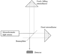
Figure 1. Simplified diagram of a freely falling cube gravimeter.
Download figure:
Standard image High-resolution image
Figure 2. An ideal solid retroreflector showing an entering ray, three reflections, and an exiting ray. Most such retroreflectors will have the points near the entry/exit face ground away, so the center of mass is closer to the corner than is the case for the cube shown here.
Download figure:
Standard image High-resolution image
The solution corresponding to release from position Z0 of the center of mass, with initial velocity V0 at  is
is

The velocity of the center of mass is

Given the gravitational potential in equation (1), the geodesic equations of free fall vertical motion give equation (4), but with relativistic corrections of order  that can be neglected. Also, in computing quantities such as
  terms that are of order
  or higher are neglected throughout this paper.
To fully describe the physics within the falling cube we need to introduce a transformation relating coordinates and time between the laboratory frame  , and the accelerating falling frame
  . We begin by computing the proper time τ of a reference clock at the center of mass, elapsed from the drop instant
  .
.
Let the metric tensor in the laboratory frame be:


where c is the speed of light at  determined with the aid of an atomic reference clock. The potential is assumed to be static in the laboratory frame during the time required for one drop. The fundamental scalar invariant is

We have adopted the metric signature  so
so  ; repeated Greek indices are summed from 0 to 3, except that only two components of the metric tensor need to be considered. Transverse motion is neglected in this paper; we do not consider Coriolis forces or rotation of the retroreflector.
The proper time of a falling clock at the origin of cube-fixed coordinates is then

where here and throughout the paper we keep the leading relativistic correction terms of order  , but keep only the contributions linear in γ.
This has an application to atomic fountain clocks, since equation (10) applies to an atom launched upwards. For atomic fountains, we neglect γ. Suppose an atom is projected upwards from  with velocity V0 sufficient to reach height H, with
  . A total time
  is required for the atom to fall back down to the starting point. During this interval the proper time elapsed on the atom from equation (10), is
The ratio of the relativistic part of this, to the non-relativistic part, is just the fractional frequency shift of the hyperfine splitting of the atom, due to relativistic effects, and is
Including γ in this calculation yields only tiny additional corrections.
Equation (10) for the proper time can be solved for T in terms of τ at the center of mass by iteration:

As can be seen, the derivations are straightforward but the expressions are algebraically lengthy. Therefore the complete calculation of the transformation equations, including the transformation function  , is provided in appendix A and we proceed mostly by quoting the results of those calculations.
In addition to the terms in equation (13), there is a correction  arising from the relativity of simultaneity. Adding this term (see appendix A) gives the net time transformation

The symbol τ is reserved for the proper time on an ideal clock at the origin of falling coordinates, while t represents the time variable extended to the region including the interior of the retroreflector, the vertical arm of the interferometer, and the beamsplitter. At the center of mass,  and
and  .
.
The transformation for coordinate  is derived in appendix A and is

It is shown in the appendix A that these transformations eliminate the term in g in the gravitational potential in the falling frame, with a small contribution remaining from the gravity gradient; in the falling frame the gradient contribution to the gravitational potential is  where z is measured upwards from the center of mass. The term
  is precisely the contribution needed for the cube to remain unaccelerated in the falling frame. The inverses of these transformations are given in appendix A.
4. Signal phase and propagation speed
The output signal of the gravimeter can be analyzed in several ways. One way is to follow the frequency from source through the beamsplitter, through the cube and back down to the beamsplitter where it is combined with the reference beam. Another way is to follow the phase of a monochromatic signal through the apparatus. Another way is to imagine sharp pulses emitted from the source, and to calculate the propagation time to the recombination point. One useful fact in such analyses is, because the gravitational field is static, coordinate frequency during propagation up or down through the gravitational field is conserved. Another useful fact is: the wavevector of a monochromatic wave is a null fourvector in vacuum. The approach we choose here is to follow the phase of the test signal from the beamsplitter, through the cube, and back down to the beamsplitter. This is simpler in some respects since phase is a relativistic invariant. We shall neglect dispersion and make no distinction between group and phase speeds of signals. Also, we are justified in treating propagation of signals in the cube neglecting gravitational potentials, provided that analysis is done in the freely falling frame.
In the lab, a signal propagating in a vacuum in the upwards direction is null and at each point along its path satisfies:

The coordinate speed of the signal will therefore be:

We choose the reference point to be at the beam splitter and set  there; the speed of light at this point in the lab is assumed to be the defined speed,
  m
m  . The coordinate speed of light above the reference point will be greater than c.
Suppose the angular frequency of the reference signal is Ω, and that the signal from the reference beam that stikes the splitter and is reflected up has phase  at the origin
  . The wavelength of the light will be
  . The phase propagates upwards with coordinate speed given by equation (17), and will reach height Z at time T given by

The phase of the signal at  is therefore

The signal four-vector  can be obtained from this phase by differentiation:

where  ,
,  . This is a null fourvector satisfying

The wavevector components obtained from equation (20) are consistent with equation (21) to the order  of the present calculation. In particular, the coordinate frequency
  in the lab is conserved in the static gravitational field.
5. Phase in the falling cube
We now follow the phase of the signal through the cube until it exits going in the  direction. The phase of the signal impinging on the front face of the falling cube is denoted by
  and will be

where  is the position of the face at time
  given by the transformation equations (15) and (14). This substitution naturally gives the phase entering the cube in terms of the time t in the local frame. Substituting and expanding to order
  , the signal phase at the retroreflector face is

The value of ϕ in equation (23) is labeled with a subscript 'in' since it corresponds to the phase that strikes the cube face. The phase is a relativistic invariant, so this is the phase entering the retroreflector in the local freely falling frame. In this frame (but in vacuum outside the glass) at this point, the coordinate speed of light differs slightly from c because  and the metric tensor still has gravity gradient terms. However, the difference is negligible, see (A.9) and (A.10). We shall neglect dispersion in the cube and assume that the coordinate phase speed of light in the glass is reduced by a factor
  . The phase speed is therefore

In the falling frame, the local time interval needed to reach height z going upwards is then

We denote the distance from the face at  to the corner by D. The total local time required for the phase front to propagate to the corner and back to the face is then double the amount calculated just above:

This time interval is the same for every ray entering the face normally. The phase  exiting the face is numerically equal to
  , but the local time at which the phase front exits is at a later local time. Therefore the replacement

will give an outgoing phase that represents the phase at a later t. In making this replacement, the last terms in γ in equation (26) do not contribute, to the order of the present calculation, so

Viewed from the falling frame, the phase front propagates in vacuum downward to negative values of z with a phase velocity
The local time required to propagate to  is
is

The phase field in the region below the cube is then

Substituting and expanding to order  gives
gives

This phase needs to be evaluated at the reference point  and expressed as a function of the time T. Substituting from the transformation equations equation (A.5) and (A.6) and then setting
  yields the phase to be combined with the reference phase at the splitter:

To the order of this calculation, solving the relativistic equations for the hyperbolic center of mass motion of the cube gives additional terms of order  in equations (5) and (6). These terms contribute to the transformation equations but because of their high order have no effect on the final phase, equation (33).
Not all of the relativistic correction terms are important; for example many of the terms multiplying γ are very small. Within the falling cube, z is usually no more than a few centimeters; with a nominal value of the gravity gradient at Earth's surface  , then
  and could be neglected. Nevertheless these terms are included since they may be important in other applications.
The signal is mixed with the reference signal, which has phase  , and fringes are counted. The phase difference is obtained from equation (33) by omitting the term
  in the second line. It is possible to absorb some of the terms in the cube depth D in the difference by redefining the initial position Z0, however it is not possible to eliminate all such terms and a significant effect remains, which will be discussed in Sect. 6.
The transformations between laboratory coordinates and freely falling coordinates provide alternative descriptions of phenomena, which must agree when results are expressed in terms of observables such as numbers of interference fringe counts. For example, in the above calculation of the test beam phase at the detector the calculation treated the source at  as at rest and the detector as moving. Alternatively, one may calculate the test beam phase at the detector in laboratory coordinates considering the source (the cube face) to be moving while the detector is at rest. In the latter case, however, one must take care to compute the time delay between the source and arrival at the detector accounting for the finite speed of light. This is analagous to computing the propagation time of a signal sent from a moving transmitter to a receiver at rest.
Let the face of the cube at transmission time TT be  and let the time required for the signal to reach the detector at
  at time T be denoted by
  . Then the time of transmission is determined by a retarded time:

This can be solved by iteration:

Each iteration introduces terms having one more factor of c in the denominator; convergence is rapid.
We denote the phase out of the cube as a function of TT in laboratory coordinates as  . This may be obtained by solving the equation
  from the time transformation, for t in terms of TT and substituting for t in favor of TT into the scalar, equation (28). The phase at the detector is then
The result agrees with the test beam phase at the splitter, equation (33).
5.1. Origin of time
The choice of zero of time is arbitrary; in the present work we have chosen to make  at the instant the cube is dropped, introducing initial position Z0 and velocity V0 to account for imperfections in release. Suppose instead the cube were dropped at a different instant T0. The center of mass position and velocity at this instant will be:

Solving for the original position and velocity, keeping linear terms in γ, gives

If one substitutes the replacements indicated in equations (38) into (33) or one lets  , and makes the replacements
  , then upon neglecting powers of γ higher than 1 it is found that the interference phase difference is form-invariant with respect to this change of time origin. For example, consider only the terms proportional to
  in equation (33). These are
Making the replacements given in equation (38) and keeping terms of order γ, this becomes

which is of the same form as equation (39) upon making the replacements  ,
,  . The remaining contributions in equation (33) behave similarly, as do all the terms proportional to D. This is a useful self-consistency check of the theory.
6. Dispersion and modulation
6.1. Dispersion
As the cube falls, the wavelength of laser radiation within the cube decreases slightly. This results in a change of phase velocity that is negligibly small, as can be seen from the following argument. The acceleration g acts for a time T that is only a few tenths of a second, causing the velocity to build up to  . The first-order Doppler shift of the laser wavelength within the cube is then no more than
  m. Chromatic dispersion for typical corner-cube glass is
  , [10] so
  . The change in time delay within the cube due to dispersion is negligible.
6.2. Modulation
Low-frequency modulation may be applied to the laser signal to aid in locking the laser to a frequency reference–e.g. a Rubidium oscillator. This modulation produces sidebands whose strength depends on the amplitude of the modulation. Every term in the beat frequency is proportional to the original laser frequency of the source, Ω, so both reference beam and retroreflected beam will have sidebands that undergo a chirp proportional to the frequency chirp of the main signal. We shall write the unmodulated phase of the signal  in (33) in the form

Assuming the signal is frequency modulated with relatively low frequency  , and has a small modulation index β, the modulated reference beam signal at distance x from the origin can be represented by

The electric field of the retroreflected beam may have a slightly attenuated amplitude, but will have sidebands such that

These signals are superimposed and sent into a photodiode. The measurements consist of time stamps of zero-crossings of the time varying quantity

The sideband frequencies also suffer from the frequency chirp that occurs as the cube falls and can be described by the phase function equation (33) with an appropriate frequency. However, unless the frequency modulation index is large we find there is almost no effect on the interference fringe counts.
7. Data analysis
Three data sets produced by a falling cube gravimeter were analyzed. These were characterized by differing numbers of drops, and differing numbers of zero-crossings of the interference signal between time stamps. These details are summarized in table 1.
Table 1. Description of data processed using equation (33).
| Project # | Number of drops | Number of time stamps | Number of zero-crossings between time stamps |
|---|---|---|---|
| #1 | 200 | 1200 | 1000 |
| #2 | 2400 | 1400 | 800 |
| #3 | 2400 | 1000 | 1200 |
The data were processed using the result in equation (33), with the term  in the second line omitted, and refractive index
  . An estimated value of gravity gradient
  was used for all drops; the data is not sufficiently robust to determine γ itself as the covariance matrix becomes singular if γ is included as a variable to be determined by the drop data. For each drop in each 'project', the data were first processed with
  , as though the reflection from the falling cube occurred at the cube face. The variables
  , and g were determined by the fit with a fixed value of γ. Then the data were processed with
  m corresponding to the distance from cube face to corner of a typical '1 inch' cube, and
  . (The values of D and d for the particular gravimeter from which this data were taken were not available.) None of the usual corrections such as those arising from polar motion or tides were applied since such corrections would be the same whether D was or was not included in the calculation. The value of g obtained when
  was invariably smaller than the value obtained when
  m. In fact the difference for all drops in all projects, including short drops obtained by selecting fewer time stamps, was found to be

with negligible variation. The same number arises if all terms of order  in equation (33) are neglected.
This is a significant correction, comparable to the magnitudes of other corrections such as arise from polar motion, or earth tides.
The fact that the difference  was found to be the same for all drops implies this constant difference should be derivable from equation (33). Suppose that fitting the drop data to equation (33) with
  results in values
  for these three parameters. Then suppose that fitting the drop data with
  results in the values
  . All these quantities are constants independent of T, so the two phase functions at an arbitrary value of T must match. Let us denote the phase given in equation (33) by
  . Linearizing the phase with respect to the small increments
  then upon subtracting the phase without D the difference should be identically zero. Thus we expect

Carrying out the calculation, we find neglecting terms of order  but without further approximation, that
It is remarkable that these replacements reduce both non-relativistic terms and terms proportional to  in equation (46) to negligible levels. This value of the correction to g is indeed equal to that found by fitting the data:

The changes in Z0 and V0 as given in equation (47) are similarly verified by fitting. Although equation (46) is a fourth-order polynomial involving five coefficients, the adjustment of only three quantities as in equation (47) is sufficient because  eliminates all odd terms in T. The residuals after applying the remaining two adjustments in equation (47) are proportional to
  and are negligible.
8. 'Speed of light' corrections
One of the more controversial issues surrounding measurements with falling cube gravimeters is the so-called 'speed of light' correction. Many measurement models of gravimeters of this type attempt to account for propagation delays between the instant the waves are reflected from the cube and the instant they are delivered to the detector, due to the finite value of the speed of light [5, 6]. A review of such speed of light corrections has been given in [8]. It should be emphasized that the result given in equation (33) does not require any such correction as light propagation has been fully described in that expression using relativistic principles.
Suppose one nevertheless attempts to derive a 'speed of light correction' by analogy with equation (46) by first fitting only with the leading  terms, then linearizing. To compare with earlier treatments we take
  and separate the phase contributions into
  and
and  contributions:

Let  be determined by data fitting using only
  , the non-relativistic part of the phase. Then one might expect corrections to satisfy

However, this is a fourth-order polynomial in the time having five constant coefficients and cannot be satisfied by adjusting three fitting parameters. Even if terms in  were neglected, there are still four constant coefficients. Thus it appears to be infeasible to derive speed-of-light corrections in this way. In case of a three-level schema in which only three fringe shifts are recorded at three times, one can imagine obtaining relativistic corrections by adjusting only three parameters.
In any case, such corrections are unnecessary; the full relativistic phase difference including propagation delays of light through the apparatus is available in equation (33).
9. Conclusions
The large value of the correction in equation (47), obtained from data analysis as well as from theory, supports the contention that in falling cube gravimeters, the time delay entailed by penetration of the light into the cube cannot be ignored. It also points up the need for a better value of the gravity gradient-not just a 'standard' value-at the position of the apparatus, as well as a precise value for the refractive index of the glass and an accurate position for the center of mass. No additional 'speed of light' correction is needed in this picture, as relativistic corrections including Lorentz contraction of the falling cube, dependence of the coordinate speed of light on gravitational potential, relativity of simultaneity, propagation along null geodesics, and first- and second-order Doppler shifts have been accounted for. The correction for time delay within the falling cube has been shown to be several microgals and to depend on properties of the cube; this correction can simply be added to other relevant corrections that are commonly applied.
Acknowledgments
We thank Tim Niebauer and Derek van Westrum for discussions and many suggestions. We are especially indebted to Tim for providing data for 5000 drops from a falling-cube gravimeter.
Appendix A. Coordinate transformations
The prescription for constructing accelerated cube-fixed normal Fermi coordinates that cover the falling cube, extending to a space-time patch containing the cube and beamsplitter, is developed in [1]. Normal Fermi coordinates[2–4], similar to Cartesian coordinates falling with the cube, are constructed by parallel propagation of a tetrad of orthonormal four-vectors along the trajectory of the freely falling test object. In the present case the trajectory is that of the center of mass of the falling cube. The 0th member of the tetrad is just the four-velocity, tangent to the trajectory of the center of mass. The time in the falling frame is the proper time on an imaginary ideal atomic clock carried along at the center of mass. The other members of the tetrad are obtained by solving equations for spacelike geodesics that intersect the trajectory of the center of mass orthogonally. In the present case the only additional coordinate of interest is the Z-coordinate so only two members of the tetrad are relevant: these are the 0-member of the tetrad tangent to the center of mass trajectory, and the spacelike 3-vector directed along the vertical Z-axis. The construction yields the following expression for the time transformation (equation (A.12) in [1]):

The integral has already been calculated in equation (13). The last term in equation (A.1) representing relativity of simultaneity is

where to the order of the calculation T can be replaced by t in equation (A.2). Combining equations (13) and (A.2) gives the transformation from time in the lab to the falling coordinates in the cube, equation (14).
We also need the transformation of vertical coordinates from the lab coordinate Z to the cube-fixed coordinate z, which is given by (equation (A.10) in [1]):

Here quantities such as  and
and  are evaluated at the cube's center of mass, which is the origin of locally inertial, freely falling coordinates. Then T is replaced by its value at the center of mass given by equation (14). The acceleration
  of the cube is obtained by differentiating equation (6). The first term in equation (A.3) is the accelerating value of the
  coordinate at the center of mass. The coefficients of z include a change of scale arising from the earth's gravitational potential, a Lorentz contraction term, and additional acceleration contributions. These contributions arise during construction of normal Fermi coordinates, while solving for spacelike geodesics that intersect the trajectory orthogonally [1]. In General Relativity, arbitrary coordinate transformations are allowed; of course then the physics in the resulting coordinate system must be interpreted in terms of coordinate-independent observables.
After expanding equation (A.3) to order  , the transformation for the Z coordinate is

The relativistic correction terms are easily identified by the factors of c in the denominators. The inverses of these transformations, obtained by an iterative process, are


These transformations can be used to investigate transformations of laser light wavevectors from the laboratory frame to the cube frame. Partial derivatives such as

where  and
and  can be easily evaluated from the polynomials given in equations (14) and (A.4). For example, the time-time-component of the metric tensor in the falling frame will be
Carrying out the partial differentiations and evaluating equation (A.8), expanding to order  , keeping linear contributions in γ, and quadratic contributions in z, we obtain

A similar calculation gives:

There are no linear terms in  or
or  in the local
  coordinate because the origin was chosen to be at the point where the net force acts. In the cube-fixed frame the center of mass is at
while the force per unit mass at z is proportional to  . The total force is then proportional to

so the retroreflector is unaccelerated in the local freely falling frame. If one should choose the flat face of the falling object as origin of the local frame, the local metric tensor would have linear terms in z.
Such features express the equivalence principle: in a freely falling reference frame, the linear term in the expansion of the gravitational potential is cancelled by terms arising from the acceleration. This is primarily an algebraic consequence of the simultaneity term equation (A.2) that was added into the time transformation equation (14). The time derivative of this term is proportional to the acceleration of the origin of falling coordinates, times a; in carrying out the standard tensor transformations of the components of the metric tensor, this term cancels the linear term in the Taylor expansion of the gravitational potential.
Although one may have questions about the transformations quoted in equations (14) and (A.4), the result clearly describes the physics in a freely-falling, locally inertial system with a static gravity gradient, with coordinates that are locally very similar to those used in Special Relativity. The linear term in the potential involving g has been transformed away in the local frame.
Appendix B. Non-relativistic derivation of corrections
The corrections given in equation (47) do not involve the constant c explicitly, and can be derived by taking the non-relavitistic limit of the equations presented above. It is instructive to summarize the argument. For example, the difference between the time coordinates in the lab and in the falling frame can be neglected. From the transformation equations, the position of the cube face is then approximately

The phase of the signal penetrating the cube is then

The time delay during signal propagation within the cube is  so the phase of the signal leaving the cube is

where in the last term the higher-order relativistic corrections can be neglected. The time required for the signal to reach the origin  , to leading order in
  , is
, is  , so the phase of the signal at the detector is
Replacing Ω by  , the 'nonrelativistic' contributions to the phase are

The first term is removed by interference with the reference beam so the net nonrelativistic phase difference is

Combining this with equations (B.1) and (5) and rearranging terms gives the phase difference

In particular, the constant term gives rise to the correction in the first line of equation (47). This correction inserted into the T2 term in equation (B.7) then leads to the last line of equation (47). The remaining terms have no effect on the conclusions stated in equation (47).
Footnotes
- *
Work of the US government, not subject to copyright.