

Abstract
Finding the stiffness map of biological tissues is of great importance in evaluating their healthy or pathological conditions. However, due to the heterogeneity and anisotropy of biological fibrous tissues, this task presents challenges and significant uncertainty when characterized only by single-mode loading experiments. In this study, we propose a new theoretical framework to map the stiffness landscape of fibrous tissues, specifically focusing on brain white matter tissue. Initially, a finite element (FE) model of the fibrous tissue was subjected to six loading cases, and their corresponding stress–strain curves were characterized. By employing multiobjective optimization, the material constants of an equivalent anisotropic material model were inversely extracted to best fit all six loading modes simultaneously. Subsequently, large-scale FE simulations were conducted, incorporating various fiber volume fractions and orientations, to train a convolutional neural network capable of predicting the equivalent anisotropic material properties solely based on the fibrous architecture of any given tissue. The proposed method, leveraging brain fiber tractography, was applied to a localized volume of white matter, demonstrating its effectiveness in precisely mapping the anisotropic behavior of fibrous tissue. In the long-term, the proposed method may find applications in traumatic brain injury, brain folding studies, and neurodegenerative diseases, where accurately capturing the material behavior of the tissue is crucial for simulations and experiments.

Original content from this work may be used under the terms of the Creative Commons Attribution 4.0 license. Any further distribution of this work must maintain attribution to the author(s) and the title of the work, journal citation and DOI.
1. Introduction
Biological tissues are complex materials that play essential roles in the structure and function of living organisms, making their characterization a crucial aspect of many fields of study [1]. The accurate characterization of mechanical properties of biological structures is vital for understanding the healthy functioning of tissues and diagnosing diseases [1, 2]. Alterations in mechanical properties, such as stiffness and elasticity, can provide important insights into disease progression, tissue damage, and other pathological conditions [3, 4]. The hierarchical and composite nature of biological tissues results in nonlinear, heterogeneous, and anisotropic mechanical behavior that making it challenging to accurately characterize their mechanical properties [5].
As a good example of a complex composite structure, human brain white matter tissue shows a highly nonlinear, anisotropic, and heterogeneous mechanical response, with a noticeable compression-tension asymmetry [6, 7]. The complex mechanical behavior of white matter tissue is attributable to the presence of stiff myelinated axons embedded within the soft extracellular matrix (ECM) [8–11]. It has been shown that finding localized stress, strain, or stiffness maps in white matter is of notable importance to many applications such as traumatic brain injury (TBI), diffusive axonal injury (DAI), and neurodegenerative brain disorders [12–19]. However, most experimental studies using classical tension, compression, and shear tests report the average mechanical properties for gray and white matter within macroscopic regions of interest, without accounting for variations in localized material behavior [7, 20–27]. While the bulk material properties of brain tissue have been extensively studied through common mechanical tests [7, 27–29], it is crucial to highlight that the connection between microscale and macroscale material properties of the brain tissue, given its complex, heterogeneous, and anisotropic nature, has not been well-explored. Currently, magnetic resonance elastography (MRE) is used to quantify the in vivo mechanical properties of the brain in health and disease [3, 15, 30–35].
MRE is an imaging technique used to measure the mechanical properties of tissues, such as stiffness. It works by applying low-frequency mechanical vibrations to the tissue using external sources, such as acoustic transducers or mechanical actuators, which generate shear waves within the tissue. Magnetic resonance imaging (MRI) is then used to capture the movement of these shear waves as they propagate through the tissue. The resulting images are analyzed, and the displacement field acquired from MRE is inverted to estimate mechanical properties, such as stiffness and damping, based on the speed and behavior of the shear waves [36–39]. In recent years, significant efforts have been made to improve the estimation of brain stiffness using MRE [30, 40], with a growing focus on incorporating anisotropy into the analysis. Traditionally, MRE predominantly relied on inversion models that assumed mechanical isotropy, but recent advancements are shifting toward more accurate anisotropic modeling [41–46]. Among the various applications of MRE, the study of brain stiffness and viscoelasticity in the context of TBI and neurodegenerative diseases has garnered increasing attention [27]. Recent studies have highlighted the role of MRE in detecting subtle changes in brain mechanical properties that are often associated with neurodegenerative processes, such as Alzheimer's disease [40, 47, 48], and the mechanical impact of TBI [49]. Despite the promising advantages of MRE, there are ongoing efforts to improve the accuracy of the entire process, including imaging, wave generation, actuation frequency, acquisition strategy, physiological vibration analysis, inversion algorithms, and processing pipelines. These improvements are crucial to address reported contradictions in global and regional brain stiffness measurements, such as the reported decrease [32, 33] or increase [50] in brain shear stiffness in normal pressure hydrocephalus, or discrepancies in findings where some studies report no significant effects of age or dementia [3, 51–53], while others indicate increases with age [54] versus decreases [55, 56]. Nevertheless, considering all recent advancements in tissue mechanics, the correlation between the independent mechanical properties of the microscopic constituent elements and the composite bulk macroscopic mechanical properties of the tissue has not been understood very well.
Recent studies on the brain white matter tissue have shown that material parameters identified for a single loading mode (for example compression) cannot be used to accurately predict the realistic mechanical response of the white matter tissue under other loading modes (for instance shearing) or multiaxial loading [7]. However, a majority of prior white matter constitutive models assume isotropy or transverse-isotropy [10, 11, 57–59]. Isotropic hyperelastic material models such as neo-Hookean, Ogden, Mooney–Rivlin, Hyperfoam, Polynomial, and Arruda–Boyce [7, 23, 25, 60] have been proposed, as well as some anisotropic models [9, 61–64]. Still, all of these models define only the mechanical response of the assumed composite bulk and homogenized white matter at a macroscopic scale and cannot explicitly capture the link between the microstructural composition and the bulk anisotropic mechanical properties of the tissue. Thus, it is crucial to systematically characterize the mechanical properties of brain tissue under multiple loading modes and establish a multiscale structure-property relationship between the local microstructural composition and the bulk mechanical properties of the tissue.
In our recent study using micromechanical modeling and multiobjective optimization [65], we predicted the independent mechanical properties of axonal fibers and ECM based on seven (or six) previously reported experimental mechanical tests for bulk white matter tissue from the corpus callosum (CC) [7]. The result of the study showed that the independent mechanical properties of white matter microstructure, which have been inversely predicted from the bulk tissue using single or dual mechanical loading modes, do not adequately describe the response of the tissue under all simple or complex combinatorial loading modes [65–69]. We used a finite element (FE) representative volume element (RVE) with periodic boundary conditions to link the mechanical responses of heterogeneous bulk tissue and microscale constituents. The multiple loading modes of the bulk tissue were used to have an accurate prediction of the mechanical properties of the microscale constituents. Although the use of RVEs in the FE method (FEM) is a convenient approach for determining mechanical behavior of a complex bio-tissue such as white matter, it is computationally expensive and time-consuming.
To address this issue and accelerate the materials design process, various machine learning and deep learning (DL) algorithms [70–73] have been used to construct surrogate models of structure-property relationships for fast forward prediction. For instance, a Galerkin reduced order model was constructed to approximate the nonlinear behavior of materials with intricate three-dimensional (3D) microstructures based on proper orthogonal decomposition [74]. An active learning algorithm called Bayesian optimization was adopted to effectively explore the search space and identify suitable candidates for guiding experiments or simulations in order to accelerate materials design [75]. A 3D convolutional neural network (CNN) was used to capture the nonlinear mapping between the microstructure and its macroscale effective stiffness [76]. However, this homogenization-based 3D CNN model cannot reveal the underlying stress–strain relationships. A 2D CNN model with the U-Net architecture was trained to predict the stress field maps of fiber-reinforced matrix composite material system [77]. Principal component analysis and CNN were combined to predict the stress–strain curves of 2D binary composites [78]. A game theory–based conditional generative adversarial neural network was applied to directly predict stress or strain fields from 2D microstructure geometry [70]. Furthermore, a 3D-CNN DL model was trained to predict the anisotropic effective material properties for RVEs with random inclusions [78]. While CNN models have been successfully employed in tasks such as image analysis and segmentation of human brain white matter tissue [79, 80], they have not yet been applied to construct structure-property relationships in the same way they have for engineered materials. Recent years witnessed a significant shift in the application of DL-based brain biomechanics with emphasize the increasing the modeling accuracy. In recent years, there has been a significant advancement in DL-based brain biomechanics, with a growing emphasis on improving the accuracy of predictive models. These advancements include the incorporation of more complex geometric representations, enhanced data assimilation techniques, and the integration of multimodal imaging data, such as diffusion MRI and tractography, to better capture the anisotropic properties of brain tissue [81]. Furthermore, the development of physics-informed neural networks and hybrid models that combine DL with traditional biomechanics has led to more accurate and robust simulations of brain behavior under various physiological and pathological conditions [82, 83].
This study aims to establish a theoretical foundation for predicting the heterogeneous stiffness map of human brain white matter tissue, with potential applicability to other fibrous tissues. The first objective is to develop a technique for automatically extracting the bulk stress–strain curves of fibrous tissue, considering its microscale constituents' material properties and architecture. A 3D CNN model is trained using FE models (in the order of thousands) to extract stress–strain curves based solely on the distribution of fibers and material properties of fibers and ECM. This technique directly extracts stress–strain curves for bulk tissue with arbitrary fiber distribution and volume fraction without the need for FE simulations. The second objective is to determine the material constants of an equivalent anisotropic material model for any bulk tissue based on its stress–strain curves in multiple directions. The 3D CNN-extracted stress–strain curves, combined with a multiobjective optimization technique, are used to inversely predict anisotropic material parameters that best fit all stress–strain curves simultaneously. This results in an accurate equivalent anisotropic material model for bulk tissue with arbitrary fiber distribution and volume fraction. The final objective is to apply the developed method to imaging data of white matter to test its performance in predicting the heterogeneous stiffness map of the brain.
2. Materials and methods
2.1. FE model
2.1.1. Model reconstruction
Our first objective is to develop a technique for automatically extracting the bulk stress–strain curves of fibrous tissue, considering its microscale constituents' material properties and architecture. To train the DL model later, we constructed a base FE model of a 3D cubic composite structure composed of distributed fibers and a soft matrix as the ECM. The edge length of the cube was set at 5 mm, and the diameter of each individual fiber bundle was randomly selected within the range of 50–200 μm [84, 85], using a uniform distribution. Fibers were distributed randomly, aligned, or oriented primarily in a specific direction to account for all possible scenarios. The construction and distribution of the fibers were performed using a Python code within the Abaqus FE package. The fiber volume fraction (FVF), defined as the ratio of the volume of the fibers to the volume of the cube, varied from 10% to 30%. This range was obtained through the distribution of fibers within the matrix to avoid any overlap between fibers during the construction of the model geometry. The fibers were meshed with truss elements and embedded in the ECM using the embedded element method [86–89]. After conducting the mesh sensitivity analysis, the element size was established at 0.3 mm, as shown in figure S1 in the Supplementary Information. We used the C3D4H and T3D2 element types for the ECM and fibers, respectively. The incompressible neo-Hookean hyperelastic material properties of the ECM were adopted from our previous work [65]. For the fibers, a linear elastic material model with no-compression behavior was used. The elastic modulus and shear modulus of the fibers and ECM were assigned values of 2.28 and 0.07 kPa, respectively [65]. Figure 1(a) illustrates a model with fiber distribution inside the ECM, with and the main orientation of . By embedding the fibers within the ECM, a 3D model was created.


Figure 1. Reconstruction of the FE model and binary phase. (a) Fibers are embedded inside the ECM to create a composite structure. (b) Six uniaxial loading cases are applied to the FE model. Three tension and three compressions in x, y, and z directions. (c) A binary phase of the FE model is created. In a binary voxel, was assigned for the voxels that fibers pass through them (blue), and zero was assigned to the voxels that include ECM (red). Each binary model has () voxels.


Download figure:
Standard image High-resolution image2.1.2. Mechanical loadings
As mentioned in the introduction, multiple loading cases are necessary to precise characterization of the anisotropic material properties of soft fibrous tissue. First, a preliminary study was conducted to determine the appropriate number and type of loading cases for extracting the anisotropic material parameters of the cubes. According to the results, out of nine possible loading cases for a cubic sample (three tension, three compression, and three shear), six cases involving tension and compression in the x, y, and z directions were selected to inversely predict the equivalent anisotropic material parameters (figure 1(b)). This selection was made because the six tension and compression loading cases provided sufficient data to accurately predict the material parameters, while the inclusion of the three shear loading cases had a negligible effect on the predicted values. However, this does not suggest that shear is an insignificant loading case; rather, it indicates that the six selected cases are adequate to accurately determine the material parameters and replicate the stress–strain curves. Additionally, including shear loading for each cube in the FE models, which number in the thousands, would significantly increase the computational cost of the simulations used for training the DL model. The rationale behind this decision will be quantitatively explained in the next section, along with further details. A 20% strain was applied to each model for each loading case, and the resulting reaction forces were recorded. Then, the extracted reaction force–displacement curves were converted to stress–strain curves for each loading case. In this study, we used the engineering stress definition and used the initial area of the cube to calculate the stress. The six stress–strain curves for each model were simultaneously used to inversely predict the material constants of an equivalent anisotropic material model for each composite model (see next section). The computational cost of the FE simulations was quantified as 3.16 Service Units (SUs) per loading case, where 1 SU corresponds to running a serial job on a single CPU core for one hour.
2.1.3. Equivalent anisotropic material properties for the cubic composite model
In this section, we aimed to replace the cubic composite model with an equivalent anisotropic continuum material. To capture the large-strain and anisotropic response of the tissue, the Holzapfel–Gasser–Ogden (HGO) [90] material model was used to find the equivalent and direction-dependent mechanical properties of each FE model. The HGO material model is one of the most prevalent anisotropic hyperelastic models. The energy density function of HGO is presented by equation (1):

where is the shear modulus of the ECM, is the first invariant of the Cauchy–Green tensor, is the fiber stiffness, is the fiber nonlinearity, and can be calculated from equation (2):


where is the fiber dispersion and is the forth invariant of the Cauchy–Green tensor (). The unit vector of the direction of the th fiber family is and is the right Cauchy–Green tensor. A model with denotes a full transverse isotropy with fully aligned fibers, while is for isotropic randomly oriented fibers.


The second Piola–Kirchhoff stress equation of the HGO model (see


We also investigated the effect of including shear loading cases in the extracted anisotropic material parameters. Nine different scenarios, with varying dispersions and FVFs, were considered. The material parameters (k1, , Ax, Ay, Az) were obtained from the optimization cycle both with and without the inclusion of shear results. Although the specific parameter values varied across scenarios (table S1), it was observed that the parameters could compensate for each other, resulting in similar overall stress–strain behavior (figure S2). This compensatory effect led to only negligible discrepancies in the stress–strain results between the two cases. Figure S2 shows the stress–strain curves generated using the material parameters derived with and without shear results, demonstrating a close alignment in most cases under tension and compression in three directions. These findings reinforce the conclusion that including shear loading cases does not enhance the accuracy of predictions but does increase computational costs.

2.2. DL
2.2.1. Reconstruction of voxel-based binary model
We developed a custom code to convert each cubic composite model, including fibers and ECM, into binary phase data on regular Euclidean grids using a level-set function. This prepares the data for utilization by the DL algorithm. Figure 1(c) depicts the composite model and its associated binary phase, depicting the fiber-containing voxels alongside the surrounding ECM voxels. Initially, all voxels are set to a value of zero. As each fiber's path is traced, any voxel whose center falls within the fiber's dimensions is assigned a value of one (figure 1(c)-right image). This results in a binary voxel representation where a value of one signifies the presence of fibers, and zero represents the ECM. To ensure accuracy, the size of the voxels was selected small enough to approximately produce the same FVF in the binary model compared to the FE model (ground-truth). The voxel size was iteratively refined until the difference in FVF between the FE model with circular cross-section fibers and the discrete binary model was less than 5%. Our preliminary results showed that to achieve less than FVF discrepancy, each cubic model should be discretized by 50 elements on each edge (125 000 voxels in total). The produced binary phase model in a format of NumPy (.npy) was used to train the subsequent DL model.

2.2.2. Dataset
In this study, we trained a CNN-based DL model using generated large-scale FE models. We generated 2000 binary phase data points with varying FVF ranging from 10% to 30%, along with different fiber dispersion and main fiber orientation. Figure 2 displays the histogram depicting the distribution of FVFs across all the cases. Our preliminary results indicated that fibers have a minimal impact on the anisotropic behavior of the cubes when the FVF is low (below 12%), particularly in cases of medium to high dispersion; therefore, fewer cases with volume fractions below 12% were considered. Conversely, as the volume fraction increases, the number of cases decreases due to the challenge of distributing numerous random fibers within the matrix without any overlap between them. We categorized all FE cases into nine groups based on the FVF and dispersion. To ensure sufficient data for statistical analysis in each FVF category, we categorized cases with an FVF less than 13% as low, 13%–18% as medium, and more than 18% up to 30% as high. To categorize cases based on dispersion, we calculated the difference between the maximum stress and minimum stress in tension along three different axes. We then categorized cases based on the stress difference, considering less than 10 MPa as high, 10 MPa to 20 MPa as medium, and higher than 20 MPa as low dispersion. Using the material prediction code, we determined the actual κ for the categorized cases. Consequently, we established cases with an average κ less than 0.2 as having low dispersion, from 0.2 to 0.26 as medium dispersion, and higher than 0.26 as high dispersion. Figure 2 illustrates six models with varying dispersion levels and FVFs, including both high and low dispersion, as well as low, medium, and high FVFs. The ECM is transparent, allowing for a clear visualization of the fibers present within it. This visualization enables a clear observation of the variations in dispersion and volume fraction across the different cases. Each of the 2000 binary phase data points represents an FE model with a shape of , in total of 125 000 voxels, where each voxel is assigned a value of either 1 or 0. The corresponding labels for these binary phase data points are stress–strain curves obtained from six loading cases applied to the model along the x, y, and z directions. More specifically, each binary phase has corresponding stress–strain curves resulting from three compressive and three tensile loadings applied along each of the x, y, and z directions.


Figure 2. Histogram of fiber volume fraction (FVF). Cases with (a) low FVF and low dispersion, (b) low FVF and high dispersion, (c) medium FVF and low dispersion, (d) medium FVF and high dispersion, (e) high FVF and low dispersion, and (f) high FVF and high dispersion. Definitions: Low FVF (FVF < 13%), Medium FVF (13%< FVF < 18%), High FVF (18%< FVF < 30%), low dispersion (κ < 0.2), medium dispersion (0.2 < κ < 0.26), high dispersion (κ > 0.26).
Download figure:
Standard image High-resolution image2.2.3. Architecture of 3D Resnet model
We adopted a 3D Resnet to predict the strain–stress curve using simulation data from the FE models. Resnet [91] is a well-established DL structure that has demonstrated remarkable success in tasks such as image processing, recognition, and classification. Unlike conventional DL models, which may encounter issues such as gradient dispersion or explosion when simply increasing the number of layers, the Resnet architecture incorporates shortcut connections to directly pass input to the subsequent layers. This approach effectively mitigates problems associated with gradient dispersion or explosion when dealing with deeper networks. To process the binary phase data and predict stress–strain curves, we utilized a pretrained 3D CNN model called Resnet18 [91]. This model, originally pretrained on the ImageNet dataset [92], which contains 2D images, provides generalizable feature representations that are transferable to 3D tasks. By fine-tuning the pretrained ResNet18 model on our brain white matter dataset, we adapted it for constructing structure-property relationships, thereby improving its performance and reducing the required training time. The Resnet18 model consists of 18 layers of neural network with 4 residual blocks (Resblocks). Each Resblock comprises four 3D convolutional layers, with the first layer being a 3D convolutional layer and the last layer being a fully connected layer. Additionally, each convolutional layer is followed by an activation layer and a pooling layer. The convolutional operation utilizes 3D filters with a size of , while the pooling operation uses filters. To introduce nonlinearity, the activation layer employs the rectified linear unit activation function, , which performs an elementwise nonlinear transformation. As depicted in figure 3, the 3D Resent takes the binary phase model as input; the output channel for each Resblock is 64, 128, 256, 512. The fully connected layer receives the output tensor from the previous layer and maps it to the desired output, corresponding to the ground-truth stress–strain curve. The detailed architecture of this model is illustrated in figure 3.


Figure 3. The architecture of the 3D Resnet model.
Download figure:
Standard image High-resolution image2.2.4. Training of the 3D Resnet model
The 3D Resnet model was implemented with PyTorch framework in python program language. The input data has a shape of 50 × 50 × 50, and the output shape is 66 × 1, which represents stress–strain curves under six different loading conditions, with each loading condition containing eleven data points (11 × 1). Here the mean squared error (MSE) loss function was adopted for minimizing the difference between the model's output and corresponding stress–strain labels, as shown in equation (3):

In equation (3), denotes total number of samples, indicates the index of six different loading cases, is ground-truth stress value and is predicted stress true value.


To assess the effectiveness of the proposed model, a total of 2000 FE models were used for both training and testing. The dataset was divided into three distinct subsets, with a distribution of 60% for training, 20% for validation, and 20% for testing. The training dataset was used to optimize the model's parameters, while the validation dataset was employed during training to fine-tune the model's hyperparameters and monitor its performance. The unseen test dataset, comprising entirely independent data that was not used during the training or validation phases, provided an unbiased evaluation of the model's generalization capabilities. This separation of data ensured that the model's performance metrics were not influenced by overfitting to the training or validation data, offering a reliable assessment of its predictive accuracy on new, unseen cases. Prior to model training, all the training data and their corresponding labels were normalized to ensure consistency and enhance convergence. To optimize the prediction accuracy of the model, we employed a technique called Ray Tune [93] for hyperparameter optimization, ensuring the attainment of the best possible results. To achieve this, we first constructed a list of potential values for two key hyperparameters: learning rate and training batch size, which are [, , , , ] and [5, 10, 20, 40], respectively. Additionally, the maximum training epoch was set at 200. It is worth noting that Ray Tune incorporates an algorithm known as Asynchronous HyperBand Scheduler (ASHAScheduler) [94] that can early stop certain training sessions whose performance has limited improvement after certain epoch. The main objective of ASHAScheduler is to identify and terminate underperforming trials (i.e. configurations of hyperparameters) early, thereby saving computational resources and time. If a trial is not among the top performers in its bracket after a certain checkpoint, it is stopped early. This decision is based on the trial's accuracy. As summarized in table S2 in the supplementary information, we conducted a rigorous exploration of hyperparameters for 3D Resnet by sampling 20 different training sessions from the high-dimensional search space. Each session was assigned specific learning rates and batch sizes, and the optimal hyperparameters were determined with the assistance of Ray Tune. Session 13 emerged as the standout performer, with a learning rate of and a batch size of 40. Training the DL model required 200 epochs, with a total training time of 5021.8 s on two NVIDIA GeForce RTX 3090 GPUs. Once trained, however, the DL model offers a much more efficient alternative for evaluation, taking only 5.86 s per test case. This represents a significant speed-up of approximately 1940 times compared to the FE simulation for each evaluation.


2.3. Application of the FEM-based DL model for predicting white matter stiffness map
The developed method was used to demonstrate its effectiveness in predicting the stiffness map of a localized region within the human brain white matter. We aimed to map the stiffness landscape of a small part of the white matter tissue by dividing it into homogenized cubes with equivalent directional properties individually determined according to the tissue microstructure by using the developed DL model. To accomplish this, a fiber tractography of a human brain segment measuring mm was used as shown in figure 4.


Figure 4. Fiber tractography of a human brain and the selected region for material characterization. The region is 10 × 10 × 10 mm which includes eight cubes with 5 × 5 × 5 mm.
Download figure:
Standard image High-resolution imageTo construct the fiber tractography, we used diffusion tensor imaging (DTI) data as follows: Initially, skull-stripping and eddy current corrections were applied to the DTI data. In diffusion spectrum imaging (DSI) Studio, a model-free generalized Q-sampling imaging method was employed to estimate the diffusion density of water across different orientations. A multi-shell diffusion scheme was utilized, with b-values of , , and , and diffusion sampling directions for each shell. The in-plane resolution and slice thickness were both set to . Restricted diffusion was quantified using restricted diffusion imaging [95]. For data reconstruction, generalized Q-sampling imaging was performed with a diffusion sampling length ratio of . Fiber tracking was conducted using a deterministic streamline tracking algorithm, enhanced with additional strategies to improve reproducibility [96]. Anisotropy thresholding was applied within a random range of – using the Otsu method. Tracks were filtered to fall within a length range of to mm, and a total of seed points were used for tracking.


Using the multiple points provided by the fiber tractography for each fiber bundle, the fiber bundles were modeled with truss elements pathing through these points. We evaluated all the fiber bundles within the designated area and assigned them random diameters falling between 50 μm and 200 μm. Subsequently, we calculated the minimum distance between these fiber bundles. If any two fiber bundles overlapped, one of them was randomly removed to eliminate the overlap. This approach resulted in varying FVF values across different parts of the specified region. Given that our trained model dimension was set as a mm cube, a total of eight separate cubes were obtained alongside a mm model. Binary phase data was generated for each cube, and the stress–strain curve was predicted for each of them. These predicted curves are then used to derive a set of material parameters, enabling the most accurate prediction of the mechanical behavior of the cube under six distinct loading cases. In conclusion, the stress–strain data of a mm model with eight different material parameters for each region, under six loading cases, was compared to the stress–strain curves of the mm model with fiber bundles. This comparison serves to demonstrate that our approach allows us to replace the complex composite tissue model, including both axonal fibers and ECM, with an equivalent anisotropic continuum material and create a compatible model without the need for an enormous number of fibers in our simulation. The assembly of the anisotropic response of all the cubes in an anatomical region can produce a stiffness map.


3. Results
Our aim was to develop and train a surrogate DL model for the FE composite model, allowing us to predict the stress–strain curves of the composite structure and provide the material constants of an equivalent anisotropic material characterized by six loading cases simultaneously. By discretizing a large and complex composite structure, such as white matter, into smaller composite cubes and replacing the anisotropic material model for each cube, we can assemble those cubes to create a stiffness map of the structure. In this section, we present the results of the proposed integrated FEM-DL framework, as well as its performance and potential applications.
3.1. FE results
Figure 5 presents a comparative analysis of the mechanical behavior of different composites under the influence of fiber dispersion, fiber main orientation, and FVF. Nine distinct cases are depicted in a 3D view to visually represent the variations in FVF, dispersion, and main orientation of fibers. Additionally, the figure includes stress–strain curves for each case under six uniaxial loadings, providing insights into the effects of these factors on the mechanical response of material.

Figure 5. Stress–strain curves for nine distinct FE composite models subjected to six loading cases. The first row presents stress–strain curves for models with an FVF of 11% and varying levels of dispersion (low, medium, and high). Similarly, the second and third rows exhibit corresponding results for models with 15% and 20% FVF, respectively. The colors blue, red, and green correspond to the x, y, and z directions, respectively. Definitions: Low FVF (FVF < 13%), Medium FVF (13%< FVF < 18%), High FVF (18%< FVF < 30%), low dispersion (κ < 0.2), medium dispersion (0.2 < κ < 0.26), high dispersion (κ > 0.26).
Download figure:
Standard image High-resolution imageThe first row of figure 5 presents three cases with a fixed FVF of 11%. Progressing from left to right, the dispersion of fibers increases, with the leftmost model representing nearly aligned fibers, and the rightmost model depicting a random distribution of fibers. Analyzing the stress–strain curves, it is evident that in the model with aligned fibers (left model), the stress in tension along the fiber direction ('X') is notably greater compared to the other two uniaxial tension directions. Conversely, when comparing compression along the fiber direction, the stress is lower than in the other two directions. This behavior is attributed to our assumption that fibers, modeled as truss elements, are incapable of bearing compressive stress. Consequently, in compression loading conditions along the fibers, the fibers do not carry any load due to their lack of compressive properties. However, in compression loading conditions transverse to the fiber orientation, the incompressibility of the ECM leads to tensile loads being applied on fibers, resulting in higher stress in these loading conditions.
The models are arranged in increasing order of FVF from top to bottom (11%, 15%, and 20%). In the first column, it is evident that enhancing the FVF significantly increases the stress in tension along the fibers, as a greater number of fibers resist tension. Additionally, the stress variation between different directions is more pronounced in the model with a higher FVF. These observations hold true in models with medium fiber dispersion as well (0.2 < κ < 0.26), but the magnitude of variations is comparatively less in these cases. In all cases with a high dispersion of fibers (κ > 0.26), whether with a low or high FVF, the stress–strain curves exhibit consistency in all loading directions for both tension and compression. These results suggest that a tissue characterized by a high fiber dispersion demonstrates isotropic behavior under both tension and compression. The variations observed between tension and compression behaviors can be attributed to the inherent tension-compression asymmetry concept, but apart from that, the tissue displays consistent behavior across different loading cases, whether in tension or compression.
3.2. DL results
The DL model was trained on a dataset consisting of 2000 FE simulation cases. In each case, the input was represented by a binary 3D matrix, while the output consisted of stress–strain curves corresponding to six distinct loading cases. This session achieved a remarkable minimum validation loss of . Notably, this validation loss is significantly lower than the typical values reported in similar DL approaches for structure-property predictions, where validation losses generally range from 10−3–10−2 [97, 98]. This suggests a high level of accuracy and generalization for the current model. As future work expands to more complex models and datasets, validation metrics will remain essential for evaluating model performance. The training and validation loss curves associated with this optimal hyperparameter setting are depicted in figure S3 in the supplementary information. The training and validation loss were both small and close to each other at the end of the training, meaning that the DL model was neither underfitted nor overfitted.

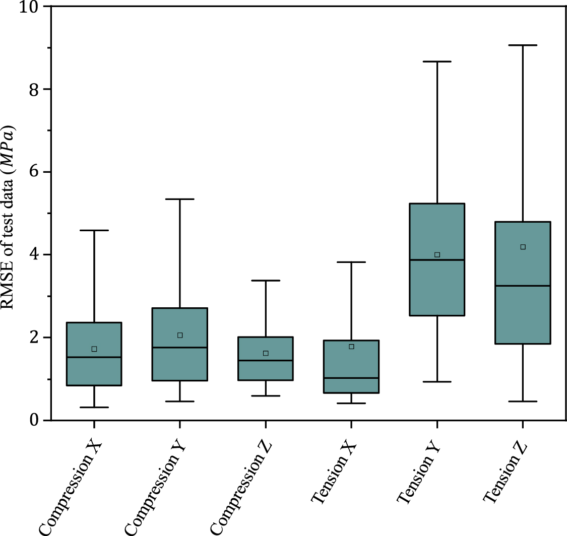
Additionally, we assessed the performance of unseen test data using checkpoints from these 20 training sessions. In this work, model checkpoints were saved every five epochs during the 20 training sessions, allowing us to preserve the model's state at different stages and select the version that performed best on the validation dataset, thus avoiding overfitting. Remarkably, session 13 consistently excelled, exhibiting the lowest test loss of , aligning with the previously identified minimum validation loss. The boxplot in figure 6 displays the distribution of RMSE of test data for different loading conditions. Here, the RMSE indicates the discrepancy between the stress–strain curves obtained from the FE simulations and those predicted by the DL model. The mean RMSEs are below 2 MPa for all compression loadings and the tension loading along the 'X' direction, whereas the mean RMSEs are below 4 MPa for tension loadings along the 'Y' and 'Z' direction. This can be explained by the greater influence of fibers under tension, given their no-compression behavior in both the HGO material model and FE simulations. As a result, predictions under compression tend to be more consistent across different cases, leading to better performance in the DL model. Beyond compression cases, the variation in RMSEs for test data under different tension directions may be due to an imbalanced training dataset. Despite applying uniform randomness for the input parameters, the dataset contained more instances with low dispersion in certain tension directions. In cases with high fiber dispersion, the fibers tend to be randomly oriented, reducing directional bias. Conversely, cases with low dispersion provide more consistent directional information, improving the model's accuracy in those specific directions.


Figure 6. RMSE between the stress–strain curves predicted by the FE simulations and the DL model for all test data across six loading cases.
Download figure:
Standard image High-resolution imageThis imbalance may affect the FEM-DL framework's generalizability, potentially limiting its reliability when applied to loading conditions that were underrepresented in the training data. To mitigate this, we plan to apply data augmentation and reweighting techniques to create a more balanced dataset in future work. These methods will help ensure that different tension directions and fiber dispersion conditions are equally represented, thus improving the framework's robustness and predictive accuracy across all scenarios. Based on the above analysis, we adopted the optimal hyperparameter configuration, comprising a learning rate of and a batch size of 40, for the subsequent DL models, ensuring the highest possible performance across the board.

Figure 7 shows the results of the DL predictions for the stress–strain curves of the three random FE testing cases. By comparing the presented results, it is qualitatively evident that the Resnet model successfully predicted the stress–strain curves under various loading conditions. Table S3 quantify the performance of the DL model in predicting the stress–strain curves of all the samples under various loading cases, FVF, and dispersion. According to table S3, and considering the overall comparison of all the test cases with varying fiber orientations and FVFs, our universal DL model consistently proves its proficiency in reliably forecasting stress–strain curves under a diverse range of loading cases. The average RMSE for all test cases is less than 4 MPa.

Figure 7. Comparison of DL and FE (ground-truth) predictions for stress–strain curves of composite models under six loading cases. (a) FVF is high (FVF = 15.2%) and fibers are highly dispersed (κ > 0.26). (b) Fibers are mainly aligned in 'z' direction (FVF = 16.9%). (c) FVF is medium (FVF = 13.9%) and fibers are mediumly dispersed (0.2 < κ < 0.26). The unit vectors representing the primary fiber orientations are displayed below each cube.
Download figure:
Standard image High-resolution image3.3. Optimization results and equivalent anisotropic material properties
The stress–strain data predicted by the DL model were used to determine the material constants of the HGO model for each individual case through an optimization algorithm. Within the HGO material model, C10 corresponds to the matrix of the composite, in equation (1). As the material properties of the matrix are the same and constant in our models, C10 is maintained at a constant value of 70 Pa [65]. Moreover, the values of D and in equation (1) were also held constant at 0.002 and zero, respectively, considering the materials incompressibility and the linear mechanical behavior of the fibers. The remaining five material parameters ( and ) were inversely estimated for each individual case, employing the stress–strain curves predicted by the DL model and a simultaneous fitting for all six loading cases.


Figure 8 presents the obtained material constants for three cases, alongside a comparison between the stress–strain curves obtained from the FE models and the optimized anisotropic material constants under the six different loading cases. Notably, the predicted stress–strain curves from the DL model were not included in this figure to emphasize the differences between the predicted equivalent anisotropic material model and the FE results. The results affirm the success and accuracy of the proposed method. By providing the composite fiber-ECM architecture, we can replace the composite model with an equivalent anisotropic continuum material, satisfying mechanical behavior in all six loading cases without the necessity of conducting further FE simulations.
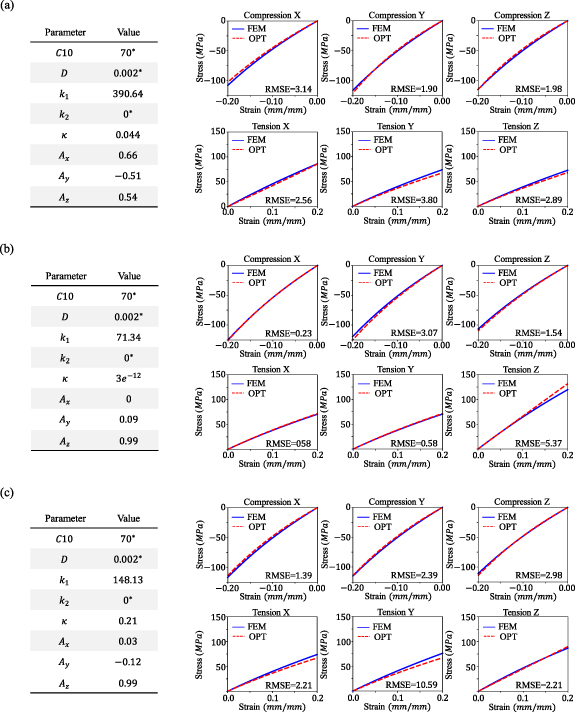
Figure 8. Prediction of the anisotropic material constants for the composite models in figure 7 using the stress–strain curves predicted by DL and inverse simultaneous fitting to the six loading cases. The figures in (a), (b), and (c) correspond to the (a), (b), and (c) figures in figure 7. The material parameters that are fixed are indicated with an asterisk (*).
Download figure:
Standard image High-resolution image3.4. Application of the FEM-based DL model for predicting the stiffness map of white matter
We applied the presented method to analyze the human brain tissue, aiming to demonstrate the efficiency and application of the method in prediction of stiffness landscape of the human white matter tissue. Specifically, we selected a region measuring mm from human brain fiber tractography and constructed two models: one with fibers and another with the predicted equivalent anisotropic material properties assigned to each cube in figure 4. By comparing the results obtained from both models, we can validate the effectiveness of our approach in accurately simulating the mechanical behavior of brain tissue while significantly reducing the complexity associated with explicitly modeling individual fibers. Since the size of the selected region is mm, eight cubes with mm dimensions are extracted in figure 4. For each cube a binary phase model cube is generated for the DL model. Figure 9 illustrates the comparison between the stress–strain curves obtained from the FE and DL models for each cube. Despite assuming straight fiber in our training data while the fiber tractography includes curved fiber bundles, we observe a remarkable agreement between DL predictions and FE results. The average RMSE of all cases is 2.59 MPa. Given that we used actual fiber tractography data, each cube exhibits unique characteristics, including FVF, main orientation, and dispersion, as depicted in figure 9.


Figure 9. Prediction of stress–strain curves for diverse cubic samples using human brain fiber tractography (refer to figure 4) and the developed DL model. The predicted stress–strain curves are compared with the stress–strain curves from the FE models (ground-truth).
Download figure:
Standard image High-resolution imageThe stress–strain curves for each cube in each loading case are obtained from both FE models and DL. The key distinction is that, in FE models, each cube requires separate analysis for each loading case, while the DL utilizes the binary model to predict the results for all loading cases instantly. The following results showcase the stress–strain curves of each cube, along with the corresponding predicted outcomes from the DL analysis. The training set focused solely on straight fibers within a specific range of FVF. In contrast, the brain model tested, based on real tractography images, includes curved fibers. This curvature, along with other potential procedural errors, likely contributes to the observed discrepancies in some loading cases. For instance, in Cube 7, the majority of fibers are curved and have an FVF of 7.83%, which falls outside the FVF range used in the training set. This mismatch likely contributes to the higher RMSE values. Despite these differences, including the presence of curved fibers and low FVF not covered in the training dataset, the method still demonstrates commendable performance. Furthermore, it is important to note that the RMSE is calculated as the sum of discrepancies across all 11 points on the stress–strain curves of the FE and CNN models, rather than a single point.
In the next step, a set of equivalent anisotropic material parameters is obtained for each cube by running an optimization cycle based on the predicted DL's stress–strain curves, figures 10(a)–(d). At the end, one model with explicit fibers (eight cubes) and one model with equivalent material properties for each cube were generated and subjected to six loading cases. In figure 10(e), the stress–strain curves of the two models under different loading cases are displayed. The results indicate an excellent agreement between the stress–strain curves of the continuum model with the stress–strain curves of the model incorporating axonal fiber bundles. The maximum RMSE between the model with fibers and the continuum model is 3.37, demonstrating the accuracy and validation of this method. This promising result demonstrates that by discretizing entire brain white matter tissue into fine voxels, determining their equivalent anisotropic material properties, and assembling them, we can create a comprehensive stiffness landscape of the human brain. This map can provide valuable insights into the local anisotropic material properties of brain tissue, addressing a current knowledge gap. Additionally, this method offers the advantage of characterizing material properties and stiffness maps across six loading cases, ensuring independence from loading mode biases present in TBI and DAI models that currently implement significantly diverse material properties. It is worth noting that, in this study, our focus was on establishing the theoretical framework and assessing its accuracy. To evaluate the performance of the proposed framework in characterizing anisotropic behavior and representing the heterogeneous stiffness landscape of brain white matter tissue or other fibrous tissues, it is essential to conduct combined experimental mechanical tests and in vitro fiber tractography of the tissue. This will be the topic of our forthcoming research.

Figure 10. Finding the stiffness map of brain tissue. (a) Fiber tractography of a human brain. (b) A random 3D region of the brain tissue, represented by a large cube, is divided into eight smaller cubes. The larger cube has an edge size of 10 mm, while the smaller cubes measure 5 mm each. (c) S11 stress contour for the large cube in (b) when it undergoes a 20% strain in the 'x' direction, including explicit fibers. (d) S11 stress contour of the continuum model with eight equivalent anisotropic material properties provided by the DL model and optimization process. For each small cube, the predicted HGO anisotropic material parameters by the DL framework are listed in the figure. For all other predefined parameters: C10 = 70 Pa, D = 0.002, k2 = 0. (e) Comparison of six stress–strain curves between the model with explicit fibers and the equivalent continuum model. The predicted equivalent continuum model, produced by the DL framework, discretizes the selected 3D region into a stiffness map using eight cubes, which accurately replicates the mechanical properties of the brain tissue including fibers. The average RMSE for all loading cases is less than 2 MPa.
Download figure:
Standard image High-resolution image4. Discussion
This study highlights the significant potential of combining FEM with DL to establish a connection between structure and properties in soft fibrous tissues. By adopting equivalent anisotropic and continuum material properties across multiple loading cases simultaneously and leveraging DL, we can accurately predict the material properties of complex composites without explicitly modeling numerous fibers. Understanding the multiscale mechanics of structure-property linkages is crucial to developing unbiased models for accurate predictions of skin aging [99], brain folding [100–104], DAI, TBI, neurosurgery [105–107], and neuroglial disorders. This study established a new multidisciplinary framework to link the mechanical properties across the scales. This is important as accurately determining the mechanical properties at a local level has the potential to enhance both sensitivity and specificity in diagnosing diseases, given that numerous neurological disorders often originate in specific localized areas or exhibit distinct regions of tissue damage. It has been shown that finding localized stiffness map in white matter is notably important for the study of neurodegenerative brain disorders [15–18]. For example, global or local reductions in brain stiffness have been reported in those afflicted with Parkinson's or Alzheimer's diseases [16, 17, 30, 48, 108].
It is worth noting that the proposed method is still in the early stages of development. To advance and validate the theoretical framework for practical implementation in biomedical applications, additional experimental tissue testing and imaging studies are essential. One direct application of the current-stage proposed method could be in simulating of DAI and TBI. Recent brain injury models have transformed fiber tractography data into FE models with explicit representations of fiber bundles as physical entities [13, 109–112]. Hence, the proposed method can be implemented to convert models with explicit representation of fiber bundles into an assemblage of voxels, each with distinct anisotropic material properties, similar to figure 10. The produced model can resolve any potential singularity or excessive shear issues regarding the fiber-ECM interaction and may save computational time for finding the global or local deformation or stress field. In this study, we used a cubic voxel with an edge length of 5 mm to train the DL model and discretized the white matter tissue. However, any smaller edge lengths can be used depending on the requested resolution and the resolution of imaging data. It is worth noting that in this study, we only discussed the hyperelastic material properties, while for DAI and TBI applications, the viscoelastic material properties should also be provided. A similar methodology to the one presented can be used to find the viscoelastic properties of the bulk tissue based on the viscoelastic material properties of fibers and ECM. The viscoelastic material properties of the fibers and ECM can be provided with a set of Prony series [66, 113] in the FE simulations to ultimately train a DL model.
Currently, contemporary models mainly define the response of the composite bulk and homogenized white matter at macroscopic scales but fail to explicitly capture the connection between the independent material properties of microscopic constituents and bulk mechanical behavior. Moreover, the implemented material models, based on a single mode, cannot accurately replicate tissue responses in other loading modes [7, 65]. Therefore, it is not surprising that multiscale biomechanical models of the brain implement mechanical properties which vary widely; in some cases by up to two orders of magnitude [12, 13, 84, 111, 114–117]. As a result, current biomechanical models simulating white matter tissue for various applications are intrinsically limited by the multiscale material properties employed. These challenges are not limited to brain tissue alone but are widespread across many hierarchical and connective tissues, including skin [118], muscle [119], ligaments [120], arteries [121], heart [122], and intervertebral discs [123]. The proposed framework is a powerful tool to study the heterogeneity in the mechanical properties of the tissue as it counts the FVF and the orientation of fibers. For example, significant heterogeneity has been observed in CC of the brain white matter where the genu, body, and splenium exhibit different stiffness [124]. This heterogeneity is not limited to CC, and heterogeneous mechanical properties have been observed in the corona radiata (CR) of the white matter as well [124]. This heterogeneity mainly stems from the differences in fiber density, fiber diameter distribution, and fiber orientation distribution. The CC has shown significantly higher storage modulus than the CR according to the MRE data [124]. The fibers of the CR, extending laterally from the CC, exhibit a lower degree of stiffness compared to the CC, where the fibers are presumed to be densely packed within its highly organized arrangement [124]. Our models also confirm that any change in the FVF, alignment, and dispersion of fibers alter the mechanical properties.
More recently, MRE has successfully integrated anisotropy considerations to derive the stiffness map of the brain. An incompressible, transversely isotropic material model with three parameters has been used to characterize anisotropic fibrous tissues, including brain white matter [125, 126]. It has been demonstrated that precise parameter estimates depend on having multiple shear waves with different propagation directions to account for directionality effects [127]. Therefore, multi-excitation MRE has been introduced and used as a promising technique for anisotropic inversion [41, 125]. Similar to multi-excitation MRE, our proposed method uses multiple loading cases simultaneously to predict equivalent anisotropic mechanical properties. However, the proposed method predicts the tissue response based on the material properties of the tissue constituents and their architecture. Among various inversion methods of MRE [128–130], the FE-based, transversely-isotropic nonlinear inversion [130] algorithm has shown great promise in recovering accurate heterogenous parameter fields and repeatable property estimates for in vivo human brain [44]. Very recently, using this method, longitudinal anisotropic mechanical properties of the minipig brain were estimated from displacement fields and DTI's fiber directions [131]. The study revealed that the white matter is stiffer than gray matter in shear in any plane containing the fiber direction and in tension in any direction with a component of fiber direction. A current challenge in predicting the anisotropic material properties of brain tissue, through the synergy of MRE and DTI, is that the used material model captures the behavior of a material with a single dominant fiber direction. This results in parameter estimates that can be inaccurate or challenging to interpret in regions with crossing fibers [131]. This so-called 'crossing-fiber' problem cannot be adequately described using the diffusion tensor model [132]. DTI assumes a single primary orientation of fiber bundles in each voxel, leading to difficulties in accurately representing areas with crossing or branching fibers. Similar to MRE, our proposed model can also be affected by this limitation as it uses DTI data for the construction of fiber paths. Recently, advanced diffusion imaging techniques, such as high-angular-resolution diffusion imaging and DSI, have been developed to address this limitation [133–135]. These techniques enable a more detailed characterization of complex fiber orientations and provide a more accurate representation of fiber crossings. Consequently, integrating the proposed framework or MRE with fiber tractography from advanced diffusion imaging methods can improve method accuracy. In this context, recent studies have investigated shear wave propagation in HGO material models with one [136] or two fiber families [137] to evaluate MRE's potential for estimating HGO model parameters from experimental data. These studies demonstrated that shear wave speeds are influenced by the HGO material parameters as well as the direction and amplitude of pre-deformations. As a result, it is feasible to noninvasively estimate anisotropic material parameters in vivo using experimental shear wave imaging data.
The advantage of predicting the stiffness map using the proposed framework lies in its ability to simultaneously quantify material parameters across six loading cases. Furthermore, the method can be readily extended to include shear loading models. This approach, which directly and automatically predicts bulk tissue anisotropy based on microscale architecture and properties, lays the foundation for an innovative framework for the inverse prediction of the architecture and material behavior of microscale constituents according to multiple loading modes of bulk tissue [65, 138]. The inverse framework has potential to address the long-lasting challenges of direct testing of microscale constituents. The direct testing methods, such as atomic force microscopy, are facing several challenges in characterization of small scale constituent, because they typically: characterize the material properties only for small deformations [139], without consideration of anisotropy [140, 141]; characterize the material property only by a single mode of loading; perform tests on components that are taken out from the natural environment [142]. The material property of the separated component from ECM can be very different from when they are embedded in ECM [143–148]. It is critical to characterize microstructure material properties when they are in their host environment [149]; consider simplified equations and assumptions such as Poisson's ratio as 0.5 [139]. The need for multiple or combined loading modes for the material characterization of soft fibrous tissues is not limited to the brain white matter tissue. As an example, the myocardial tissue of the heart [150, 151], as a complex composite tissue, displays an orthotropic material behavior. Recent experimental studies, employing either simple shear or biaxial deformations, underscore the orthotropic nature of the tissue and highlight the limitations associated with biaxial tests [152, 153]. Therefore, to establish a more comprehensive framework, it is crucial to note that relying solely on biaxial data is insufficient for an adequate characterization of the mechanical response of fibrous orthotropic/anisotropic tissues. To accomplish this task, a broader range of data, including a combination of shear and bi/triaxial extension data [154], is needed for a better understanding of the direction-dependent material behavior of soft fibrous tissues such as the myocardium and brain.
Another key advantage of the proposed method is its flexibility and adaptability. By employing a binary phase representation (or multiple phases), the method can model any anisotropic tissue with diverse microscale components, including different geometries such as spherical shapes rather than slender ones. The approach allows for discretizing and representing any geometrical features with discrete voxels. Moreover, it can be adapted to explore regional differences within the same tissue by modifying the material properties and geometries of its microscale constituents. Consequently, this method is broadly applicable to any composite tissue, irrespective of the specific tissue type being modeled. Therefore, as the HGO model has been previously used for multiscale modeling of myocardial tissue [152, 153], the proposed framework in this study can be adapted and used in accordance with available experimental data with multiple loading modes [154–157].
In summary, our work paves the way for accurately and rapidly predicting stiffness maps in the human brain or other connective tissues by capturing the complex, nonlinear, and asymmetric material behavior of tissue microstructure. By integrating FEM and DL, we contribute to the ongoing advancements in computational tissue mechanics, opening doors to a deeper understanding of brain mechanics and its implications in various neurological conditions.
5. Limitations and future work
In this study, similar to other computational simulations, there are multiple inherent simplifications and limitations. While we currently divided the tissue into two components, axonal fibers and ECM, it is worth noting that other constituents, such as glial cells [158], can also influence the material behavior of brain tissue. Nonetheless, the proposed method is highly adaptable and can be expanded to accommodate multiple microscale constituents with varying mechanical properties. This approach is not limited to fibrous tissues and can be applied to model composite tissues with constituents of different shapes. The method used to prepare the binary phase can be readily employed for various composite tissues. The FVF of the models ranges from 10% to 30% to prevent fiber intersections. However, it is known that in soft fibrous tissues, the fiber density can be significantly higher. Nevertheless, the performance of the proposed framework performance remains unaffected, and it can effectively model tissues with varying FVFs by providing the binary map. To determine the stiffness map of brain tissue, we calculated the FVF of each cube based on the number of fiber tracts obtained from fiber tractography and a random fiber diameter ranged from 50 to 200 μm. In reality, the FVF of each cube or discretized voxel should be derived from experimental histology or imaging data. Studies have demonstrated that FVF can be calculated from fractional anisotropy for fully aligned fibers [159]. Additionally, there exists a relationship between fiber dispersion and fractional anisotropy that should be applied in practical scenarios [64, 160].
In this study, to determine the equivalent anisotropic material properties for each composite cube, we held the material properties of the ECM constant and assumed that the anisotropic behavior of tissue resulted from variations in the FVF, orientation, and dispersion of fibers. However, in reality, the mechanical properties of the ECM may also vary based on the microscale constituents and anatomical location. We conducted the optimization step outside of the DL framework for the sake of simplicity. However, it can be conveniently incorporated into the DL model by adding another loss term of mechanical properties to create a unified framework.
In this study, we used a cubic voxel with an edge length of 5 mm to train the DL model and discretized the white matter tissue. We selected 5 mm cube to facilitate future comparative studies based on recent mechanical tests conducted on bulk brain tissue [7]. However, smaller edge lengths can be employed based on the requested resolution and the resolution of imaging data, considering that the typical resolution of MRE is 1.5 mm volumetric [42]. Hence, the edge length of the cubes can be reduced to 1.5 mm for future studies, facilitating comparison with MRE studies. While smaller edge lengths offer better representation of fiber alignment, they can increase computation time. The aim of this study was to balance accuracy and resolution.
It is important to note that the embedded element technique should be employed with caution, as stiffness redundancy increases the overall model stiffness and may lead to altered results if not carefully addressed. In the current study, the use of truss elements for fibers and solid elements for the ECM complicates the straightforward elimination of material redundancy by reducing the shear modulus of the ECM from the fibers' shear modulus [65, 66]. However, it is crucial to highlight that, in this study, the FE models and DL model, operating based on overestimated stiffness values, do not adversely affect the performance of the proposed method in predicting material properties. The impact is confined to the absolute values of the material properties. Nevertheless, for practical applications and closer alignment with experimental data, resolving stiffness redundancy should be addressed through customized methods.
In our study, the maximum applied strain is 20%, which aligns with quasi-static mechanical tests of white matter tissue [7, 161]. However, investigating the effects of varying strain levels, particularly at higher strains, could significantly impact the mechanical characterization of white matter. Increasing the strain range may introduce greater nonlinearity into the stress–strain curves, potentially affecting the accuracy of the predicted material constants. Understanding how different strain levels influence the mechanical properties of white matter is essential, especially for future applications involving diverse strain conditions or different tissue types.
In future studies, we aim to link imaging parameters like fractional anisotropy and radial diffusivity to the DL framework to enhance the practicality of our models. This will also help connect our proposed method to recent studies focused on estimating the material parameters of the HGO model from in vivo MRE imaging data [136, 137]. We will conduct combined experimental mechanical tests and in vitro fiber tractography to evaluate the performance of the proposed framework in characterizing anisotropic behavior and representing the heterogeneous stiffness landscape of brain white matter tissue.
6. Conclusion
Finding the stiffness map of biological tissues is a challenging task due to the heterogeneity and anisotropy of connective tissues. To tackle this challenge, in this study, we proposed a new method to map the stiffness landscape of fibrous tissues, specifically focusing on brain white matter tissue. To do so, a DL framework was established based on large-scale FE models of fibrous tissue under six loading cases and an optimization process. The trained and tested framework was capable of predicting the equivalent anisotropic material properties solely based on the fibrous architecture of any given tissue. The method was applied to imaging data of brain white matter tissue, demonstrating its effectiveness in precisely mapping the anisotropic behavior of fibrous tissue. This study serves as the foundation for predicting the heterogeneous stiffness map of human brain white matter tissue, with potential applicability to other fibrous tissues as well. The performance of the proposed method, which aims to link multiscale mechanical properties of real tissue, will be evaluated through tissue mechanical tests and imaging data, with a focus on potential future biomedical applications.
Acknowledgments
M J Razavi acknowledges funding from the National Science Foundation [CMMI-2123061]. M J Razavi and D Liu acknowledge the Transdisciplinary Area of Excellence (TAE) Data Science Seed Grant from Binghamton University.
Data availability statement
The data that support the findings of this study are openly available at the following URL: https://github.com/akbarsolhtalab. Data will be available from 31 August 2024.
Conflict of interest
Authors have no conflicts of interest to disclose.
Author contributions
P C: Methodology, Formal analysis, Software, Writing—original draft. GL: Methodology, Formal analysis, Software, Writing—original draft. A S: Methodology, Formal analysis, Software, Writing—original draft. D L: Investigation, Supervision, Writing—review & editing, Funding acquisition. M J R: Conceptualization, Investigation, Supervision, Writing—review & editing, Funding acquisition. All authors reviewed the manuscript.
Appendix: HGO model
The HGO model incorporates the neo–Hookean model for the isotropic ground material, while the anisotropic component includes families of fibers. Thus, the strain-energy function can be represented as [162]:

For convenience, we have separated the derivation of the isotropic and anisotropic components. The neo-Hookean strain energy function can also be partitioned into two components, representing the volumetric and isochoric responses of the material.

where μ and are temperature-dependent material parameters. is the Jacobian or the volume ratio defined as the determinant of the deformation tensor F, and is the first deviatoric strain invariant which can be derive from the principal stretches,


The second Piola–Kirchhoff stress tensor for the volumetric and isochoric can be determined by

where C is the right Cauchy–Green tensor defined as and is modified right Cauchy–Green tensor defined as . The volumetric and isochoric second Piola–Kirchhoff stress tensors can be shown in the following terms:


The strain energy function of the anisotropic segment comprise families of fibers represented by pseudo-invariants, . The pseudo-invariant represents the directions of fiber families, and the direction of these fibers are represented by unit vectors ,


where , are temperature-dependent material parameters; N is the number of families of fibers (N ⩽ 3); and '' operator stands for the Macauley bracket and is defined as . can be obtained by


Here, represents a temperature-dependent material parameter that signifies the dispersion of fibers. In our study, we considered only one family of fibers, N = 1.

The second Piola–Kirchhoff stress tensor for the anisotropic segment can be determined by


where '' represents the dyadic product. The total second Piola–Kirchhoff stress is the sum of both the isotropic and anisotropic components of the stresses.
