


Abstract
By taking the spin and polarization of the electrons, positrons and photons into account in the strong-field QED processes of nonlinear Compton emission and pair production, we find that the growth rate of QED cascades in ultra-intense laser fields can be substantially reduced. While this means that fewer particles are produced, we also found them to be highly polarized. We further find that the high-energy tail of the particle spectra is polarized opposite to that expected from Sokolov–Ternov theory, which cannot be explained by just taking into account spin-asymmetries in the pair production process, but results significantly from 'spin-straggling'. We employ a kinetic equation approach for the electron, positron and photon distributions, each of them spin/polarization-resolved, with the QED effects of photon emission and pair production modelled by a spin/polarization dependent Boltzmann-type collision operator. For photon-seeded cascades, depending on the photon polarization, we find an excess or a shortage of particle production in the early stages of cascade development, which provides a path towards a controlled experiment. Throughout this paper we focus on rotating electric field configuration, which represent an idealized model and allows for a straightforward interpretation of the observed effects.
Export citation and abstract BibTeX RIS
1. Introduction
The ongoing development of high-power petawatt class lasers [1] has already opened new avenues for high-intensity laser-plasma physics. Already with present day laser technology the effect of QED process can be observed in high-intensity laser-matter interactions [2–4]. With the upcoming generation of multi-10 PW laser systems [5, 6] it is expected that laser-plasma interactions will enter a novel regime of QED plasma physics where strong-field QED process such as high-energy photon emission via nonlinear Compton scattering and electron-positron photo-production will play an important role for the overall dynamics of the plasmas [7].
One of the most striking predictions of strong-field QED [8, 9] is the formation of avalanche-type QED cascades [10] at laser intensities approaching 1024 W cm−2. In these cascades the prolific generation of high-energy photons and electron–positron pairs can convert an initially strong laser field into a hot and dense plasma of electrons, positrons and photons. One of the conclusions drawn from these predictions was that the Schwinger field ES = 1.3 × 10¹⁸ V m−1 is then difficult to reach because of laser field depletion during the cascade [11–13].
In a cascade, efficient pair production is facilitated by hard photons which have a quantum parameter χγ ≳ 1. A particle with four-momentum pμ has quantum parameter χ = e|Fμν pν |/m3, where Fμν is the EM field strength tensor, e the elementary charge and m the electron mass. Those photons, in turn, are emitted by leptons, i.e. electrons and positrons, with χe ≳ 1, leading to exponential increases in particle number [10, 14–19]. A renewable supply of sufficiently many leptons with χe ≳ 1 necessarily can be provided if the electric field of the laser is capable of accelerating low-energy leptons with χe ≪ 1 to χe ≳ 1.
This is one of the decisive features in avalanche-type cascades, which can occur, for instance, in rotating electric fields at the magnetic nodes for two counter-propagating circularly polarized laser pulses [10, 20]. Such an avalanche-type cascade exhibits an exponential growth in particle number, limited by the available (laser) field energy. By contrast, in shower-type cascades that occur in interactions of high-energy particle with non-accelerating field configurations, such as in collisions with (nearly) plane-wave laser pulses, the leptons are not reaccelerated to χe ≳ 1, and therefore the cascade multiplicity is limited by the maximum initial particle energy [21–23].
QED pair-cascades are important in extreme astrophysical environments, where they may develop in matter, photon gas and magnetic field backgrounds [24]. In the latter case of cascades in strong magnetic fields, as found in pulsar atmospheres [25, 26], the same basic theoretical framework to describe the quantum processes is used for describing laser-plasma interactions [27]. There has been significant recent progress in understanding important physics details of cascades, including aspects of laser polarization, field structure [28–30] and seeding [31, 32].
Lepton spin- and polarization effects in strong-field QED(-plasma) processes have gained some significant recent interest [33–40], (even though some fundamental scattering cross sections in strong laser fields were calculated much earlier [41, 42]). It was shown that electron beams colliding with bi-chromatic laser pulses can self-polarize due to hard-photon emission [36], and that positrons generated by these photons are polarized as well [38]. Alternatively, it was proposed to collide electron beams with elliptically polarized laser pulses to generate polarized lepton jets [37, 39]. The radiative self-polarization of electrons in rotating electric fields in analogy to the Sokolov–Ternov effect [43, 44] was studied e.g. in [33, 34]. An interesting scenario is the impact of particle polarization on the formation of avalanche-type cascades, which may be expected to potentially be a large effect due to its exponential nature.
In this paper, we study the influence of lepton and photon spin and polarization on the formation of QED cascades. We find that the inclusion of particle polarization does affect the growth rates of cascades, and that all particle species in the developing cascades are highly polarized. Moreover, the high-energy tails of the lepton energy spectra are polarized opposite to what is expected from Sokolov–Ternov theory. In photon-seeded cascades we also find an excess of pairs in the early stages when the cascade is seeded by ⊥-polarized photons (compared to unpolarized or ∥-polarized photons), which presents a path towards an experimental confirmations of the theoretical results.
Our paper is organized as follows: in section 2 we first develop the theoretical model based on a Boltzmann-type kinetic equation with a polarization dependent collision operator. In section 3 numerical results are presented and discussed. Our findings are summarized and concluded in section 4. Technical details and background are provided in the appendix, including details on the numerical method.
2. Theoretical model
So far, in simulations of cascades only the photon polarization was taken into account in [45], but lepton polarization was neglected. That means, in each generation the leptons emit polarized photons, but without any influence from previous generations because leptons are and stay unpolarized. Here, the full polarization evolution is taken into account consistently over many generations. The laser field is described as a rotating electric field  , which is a suitable model for colliding laser pulses widely used in the literature [10, 11, 17, 18, 20, 46, 47] and is generated at the magnetic nodes of colliding laser pulses. The rotating electric field represents a simplified model of a real high-intensity laser plasma interaction which allows for a straightforward analysis of the observed particle polarization properties.
We model evolution of the polarized QED cascades by a Boltzmann-type kinetic equation [17, 18, 48, 49] for the one-particle distribution functions  of of electrons (q = −1), positrons (q = +1) and photons (q = 0), where q is the particle's charge in units of e, and in a polarization state s. The transport equations for
  in a rotating electric background field are derived in appendix
  , which is the magnetic field direction in the rest frame of the leptons. This represents a global non-precessing spin quantization axis (SQA) which means that the spin vectors of particles polarized along the z-axis do not process according to the T-BMT equation [33, 50]. (The spin-polarization components perpendicular to
  do not have to be treated explicitly, see appendix
Throughout the paper we use natural Heaviside–Lorentz units with ℏ = c =  0 = 1. We further introduce normalized (dimensionless) time ωt → t, momentum
  and electric field
  . Thus, the normalized E0 has the same numerical value as a0. For the Minkowski metric we use the sign convention (+, −, −, −).
The normalized Boltzmann equation can then be written as

where  are the collision operators describing all relevant strong-field QED processes, with the charge q labelling different particle species. The
  are linear functionals of the spin and polarization dependent differential rates for nonlinear Compton scattering and pair production [8, 45, 52, 53]. The rates were calculated from first-order high-intensity QED Feynman diagrams in the Furry picture within the local constant crossed field approximation [54–56], see also appendix
The lepton collision operators  describe the energy losses due to radiation emission and accompanying spin-flip transitions, as well as a gain term due to pair production by photons. The photon collision operator
  contains terms for the absorption of j-polarized photons during pair production and the generation of photons by non-linear Compton emission off of electrons and positrons. The explicit expressions for the polarization dependent collision operators are given below in section 2.2.
The classical advection operator on the left-hand side of equation (1) does not mix different polarization states (because of the choice of the non-processing SQA, see appendix
2.1. Characteristics
The characteristics of the left-hand-side of (1) describing the classical trajectory can be found analytically by solving the equation of motion in the rotating electric field:

which means, for leptons with q = ±1,  lies on a circle with radius a0 around the centre
  , where
  is the normalized vector potential and
  is the conserved canonical momentum. Leptons starting with zero momentum can be accelerated up to
  , where a0 = eE0/mω. For the photons, with q = 0, equation (2) is just free ballistic motion with constant momentum.
For a numerical solution of the Boltzmann equation it is convenient to introduce the angle φ between  and
and  for all particle species [17]. The equations of motion for the characteristics in terms of the new variables
  and φ read


with the completely analytical solution,


with  . Here p0, φ0 means those quantities are taken at t0. The characteristics are written in terms of the time-step Δt = t − t0. Note that equations (5) and (6) are exact to all orders in Δt. For the sake of completeness, we also write down the Boltzmann equation in the new variables:

2.2. Polarization dependent collision operators
The benefit of introducing φ becomes apparent when considering the quantum transitions; ultrarelativistic particles emitted during the quantum processes are kinematically restricted to be collinear to the emitting particle and therefore involve transitions at constant φ such that only the magnitude of momentum, p, changes. The angle φ enters the collision operator only parametrically via the quantum parameters

which determine the probabilities of the QED processes, and with the normalized Schwinger vector potential aS = m/ω.
Quantum transitions leave the momentum angle φ unchanged. This greatly simplifies the numeric calculations. The polarization dependent collision operators for electrons, positrons and photons can be written down as

The collision operators (9)–(11) are a generalization of both the collision operators to describe the evolution of unpolarized cascades [17, 18, 48, 49], as well as the collision operator for the radiative spin-polarization of electron beams [36]. They are functionals of the differential rates for nonlinear Compton scattering w±1 and nonlinear Breit–Wheeler pair production by a photon w0, as well as the corresponding total (momentum integrated) rates (see appendix

as well as the polarized one-particle distribution functions of all particle species  . We should emphasize again that these collision operators furnish transitions between different momentum of the particles, but only with regard to their magnitude. The angle φ enters only parametrically, and the quantum rates depend on φ only via their respective quantum parameters χq
(p, φ), equation (8). In that sense, these collision operators are effectively 1D (i.e. one momentum integral) because the momentum direction does not change in a quantum transition in the ultrarelativistic approximation (when collinear emission is assumed as usual). The momentum ratios, such as p/k appearing in the last term of equation (11), are reflections of this reduced dimensionality. The details of the reduction of the full 3D collision operator to the 1D ones for the rotating field case are discussed in the literature, see e.g. references [17, 18]. Let us now briefly discuss the physical meaning of the individual terms in the collision operators.
. We should emphasize again that these collision operators furnish transitions between different momentum of the particles, but only with regard to their magnitude. The angle φ enters only parametrically, and the quantum rates depend on φ only via their respective quantum parameters χq
(p, φ), equation (8). In that sense, these collision operators are effectively 1D (i.e. one momentum integral) because the momentum direction does not change in a quantum transition in the ultrarelativistic approximation (when collinear emission is assumed as usual). The momentum ratios, such as p/k appearing in the last term of equation (11), are reflections of this reduced dimensionality. The details of the reduction of the full 3D collision operator to the 1D ones for the rotating field case are discussed in the literature, see e.g. references [17, 18]. Let us now briefly discuss the physical meaning of the individual terms in the collision operators.
The first two terms in each of equations (9) and (10) describe the radiative energy loss of the leptons during photon emission, i.e. quantum radiation reaction [18, 59, 60]. These terms include both the possibility of spin-flip and non-flip transitions and thus are also responsible for the radiative lepton polarization, and they had been used already in [36]. In addition, they describe the spin-dependence of quantum radiation reaction. The last term in each of (9) and (10) is for the generation of up/down polarized electrons and positrons from photons of arbitrary polarization, respectively.
For the photon collision operator  in equation (11) the first term describes the absorption of j-polarized photons during pair production and the second term describes the generation of j-polarized photons by non-linear Compton emission from both electrons and positrons (summed over charge q).
3. Results and discussion
Numeric solutions of equation (1) for the up and down electron and positron distributions in the presence of both the quantum processes and the classical motion are shown in figure 1, for a0 = 1000 and ω = 1.55 eV. In figure 1 we also plot the χ±1 isocontours, which greatly vary over the phase space. In particular, at the lines φ = ±π/2, where the particle momentum and the electric field are perpendicular, the quantum parameters are χq
≈ a0
p/aS. A characteristic value of χq
can be defined at the fixed points, φ = −qπ/2, p = a0, of the lepton phase-spaces as  . For the parameters used in figure 1, χFP = 3.03.

Figure 1. Snapshot of the electron (a), (c) and positron (b), (c) distribution functions in an up (a), (b) or down (c), (d) polarization state for a0 = 103 and ωt = 10 in a rotating radial frame. Green curves are χ isocontours. Black dashed curves represent the separatrix of the classical advection p = −2qa0 sin φ, and black crosses are the corresponding fixed points at φ = −qπ/2, p = a0.
Download figure:
Standard image High-resolution imagePhotons are predominantly generated with ∥-polarization. Leptons of both polarization states are dominantly produced by photons that reach φ = ±π/2 because χ0 is largest there. Leptons produced at φ = qπ/2 (i.e. outside the separatrix) are accelerated to large p by the electric field as they orbit to φ = −qπ/2 and hence large values of χ±1 exceeding  . When χ±1 ≳ 1, photon emission is efficient, and therefore leptons, while they are being accelerated, are most likely to radiate photons. As a consequence, they lose sufficient energy to enter the closed orbits inside the separatrix, where they accumulate. Note that no classical orbits cross the separatrix and the quantum transitions only take leptons from outside the separatrix to inside, so once inside the separatrix, leptons are trapped. Spin-flip transitions occurring during photon emission lead to further polarization of the leptons. A movie of the evolution of the distribution functions is provided in the supplementary material (https://stacks.iop.org/NJP/23/053025/mmedia).
The shape of the distribution and their location inside the separatrix are determined by a balance of classical acceleration, feeding due to pair production, and photon emission. The latter two processes are spin dependent. Therefore, it is not surprizing that the shapes of the up and down particle distributions are different. For instance, the values of χ±1 at the maximum of the distributions are 1.04 for up electrons, but only 0.70 for down electrons. The position of the distribution's peak,  , is also an indicator for the magnitude of radiation reaction effects. In figure 1 we find a difference in the angular shift of
  , signalling a spin-dependence of radiation reaction. By treating radiation reaction semiclassically as a continuous friction force (and neglecting pair production) [61, 62], the angle deviation is proportional to the strength of the radiation reaction force in a lowest order perturbative analysis.
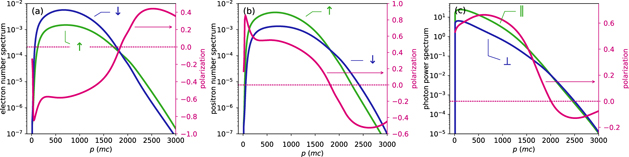
Figure 2 shows the spectra of electrons (a), positrons (b) and photons (c) at ωt = 10 for a0 = 1000, seeded by an unpolarized electron. The plots also show the degree of polarization for each case, i.e. Figure 2. Momentum spectra (blue/green curves) and differential degree of polarization (pink curve) for electrons (a), positrons (b) and photons (c). Same parameters as in figure 1. Download figure: for electrons and
  for photons. These plots show that the positron polarization is opposite to the electron polarization. Slight deviations occur because the cascade is seeded by electrons. For the leptons the main peak extends roughly up to about 2a0, which mostly corresponds to particles accumulating inside the separatrix. Those particles are dominantly polarized, as predicted by Sokolov–Ternov theory, with electrons more likely in a spin-down state (and positrons in an up-state).
  , is smaller than that for down electrons,
  , such that they are less likely to emit and hence have a larger probability to reach higher energies than down electrons. This is contrary to the explanation of the Sokolov–Ternov effect, where the difference of spin-flip transition rates
  and
and  was decisive [43].
The important findings of previous studies of cascades [10, 11, 17, 18] was that they eventually reach exponential growth in particle number, n = ∫dφdp p f ∝ eΓt . Our numerically calculated growth rates are in reasonable agreement with the analytical models of [30, 64]. The evolution of the particle yields are shown in figure 3 for an unpolarized electron seeded cascade for parameters a0 = 600 and ω = 1.55 eV. We compare a calculation of a polarized cascade with an unpolarized cascade, simulated using only unpolarized distribution functions and rates in the collision operator (see e.g. [17]). Figure 3(a) shows that the yields of up electrons decreases initially. This is because of spin flip transitions in the photon emission (Sokolov–Ternov effect). Later in the evolution of the cascade, pair production becomes more relevant and all particle yields enter an exponential growth phase, eventually reaching a common growth rate Γ. In the exponential growth phase there are 5 times more down than up electrons (opposite for positrons). Moreover, a factor of four more ∥-polarized photons are emitted compared to ⊥-polarized photons. Thus, the particle distributions produced in a QED cascade are highly polarized.

Figure 3. Time evolution of electron (a), positron (b) and photon (c) yields during a cascade seeded by unpolarized electrons, and for a0 = 600 and ω = 1.55 eV. Results for a polarized cascade are compared to an unpolarized cascade simulation.
Download figure:
Standard image High-resolution imageThe growth rate is calculated as  , with
  as t → ∞, and shown as a function of a0 in figure 4(a) We find that the growth rate of a polarized cascade when electron spin and photon polarization are properly taken into account is typically smaller than in an unpolarized cascade calculation by about 3% to 8%, with the maximum discrepancy around a0 = 600 in this case, see figure 4(b). It is worth noting that a reduction in the growth rate of ∼5% at a growth rate of ∼1 (i.e. a0 ∼ 2000) corresponds to a reduction in particle yield by an order of magnitude in less than ten (laser) cycles. For fixed laser frequency ω, the effective value of χ at the fixed point of the classical advection
  . It is also of interest to examine the behaviour at fixed
  , which is shown in figure 4(c). Here, the growth rate differences increase with increasing a0 and reach 25% for the longest wavelengths simulated, which is a considerable reduction.
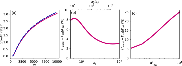
Figure 4. Cascade growth-rates Γ (a) as a function of a0 at fixed ω = 1.55 eV and the corresponding relative difference between polarized and unpolarized growth-rates (b), and for χFP = 1 = const. (c).
Download figure:
Standard image High-resolution imageThese changes in the growth rates can be traced back to the collision operators for particle species q, summed over all polarization degrees,  . The operators
  govern the quantum transitions for the distribution function of a particle species summed over all polarization states
  . We now isolate the polarization dependent terms in the collision operators
  and pinpoint the differences to the unpolarized collision operators
 used so far for the description of unpolarized QED cascades.
The unpolarized collision operators  contain only the polarization averaged rates of photon emission and pair production,

and their momentum-integrated counterparts  . Until now, only the unpolarized collision operators
  have been used in simulations of QED cascades almost exclusively, see e.g. references [17, 18, 48, 49, 59], with the exception of reference [45] where the effect of photon polarization was included. However, they represent only a part of the full collision operators when all the particle polarization is taken into account.
The derivation of the full  from the expressions in equations (9)–(11) is lengthy, but straightforward, and the final result reads


We see that the difference between the  and the unpolarized collision operators
  contain terms that couple the polarization imbalances of the lepton,
  , and photon,
  , distribution functions to the rates' polarization disparities vq
. The latter are defined as the difference of the scattering rates between the initial particle polarizations, summed over all final state polarization
, distribution functions to the rates' polarization disparities vq
. The latter are defined as the difference of the scattering rates between the initial particle polarizations, summed over all final state polarization


with s = + 1 ⇔ ↑, s = −1 ⇔ ↓, j = + 1 ⇔ ∥, and j = −1 ⇔ ⊥. Moreover, we defined the corresponding total rate disparities as, e.g. V0(k) = ∫dp v0(k → p).
In our model with polarization taken into account, the rate disparities vq couple to the particle polarizations Πq , and this affects even the polarization summed collision operators and therefore causes a change in the growth rates.
Seeding for the cascade is an important consideration [30–32]. With the methods developed here, we can also study the evolution of a QED-cascade with an initially polarized seed particle distribution to make an experimentally verifiable prediction. We choose to examine a polarized photon seed, since polarized photons could be readily generated and their polarization controlled by inverse Compton scattering [65]. The basic idea could, however, equally work with an initially polarized electron seed.
These calculations were performed with a0 = 400 and a seed photon momentum k = 103 mc, with the seed photon initially either ∥- or ⊥-polarized. Figure 5(a) shows the time evolution of the particle yields, depending on the polarization of the seed photons. It shows a significantly higher yield of produced pairs for ⊥-polarized seed photons in the early stage.
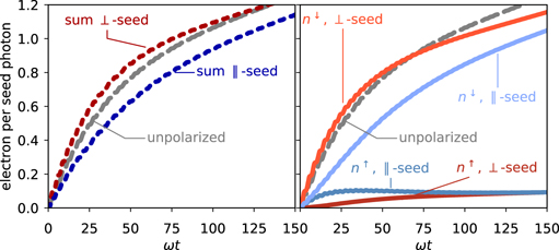
Figure 5. Time evolution of the electron yield of photon seeded cascade for a0 = 400 and seed photon momentum k = 103 mc, with the seed photon initially either ∥- or ⊥-polarized.
Download figure:
Standard image High-resolution imageMoreover, the electron spin distribution depends strongly on the seed photon polarization, see figure 5(b). ⊥-Polarized photons produce polarized pairs directly, with a very high abundance of down electrons (up positrons). By contrast, ∥-polarized photons produce equal amounts of up and down electrons and only later are they self-polarized via spin-flip photon emission. For ⊥-polarized seeds the yield of down electrons alone exceeds the total electron yield predicted in an unpolarized calculation.
These findings suggest an intriguing experimental scheme to investigate the polarization dependence in strong-field QED-cascades with soon-to-be available lasers: two counter-propagating, circularly-polarized tightly focussed 10 PW laser pulses collide and set up a standing wave. A highly polarized gamma-photon beam is injected into the magnetic nodes of the plane wave where the field is a rotating electric field. Rotating the polarization of the gamma-rays from parallel to perpendicular to the axis of the standing wave will lead to measurable variations in the particle yield, see figure 5(a).
4. Conclusions
In conclusion, we have shown that QED-cascades will lead to highly polarized particle generation and that the growth rates are reduced by the spin-dynamics, leading to orders of magnitude differences in particle yield compared with calculations with unpolarized rates under certain conditions. This raises the prospect of generating polarized lepton beam perhaps useful for laser-wakefield driven particle colliders [66], or the production of highly polarized γ-photons [65, 67]. However, addressing the fundamental role of particle polarization in QED cascades, as we have here, could have wide-ranging implications. For example, QED cascades may occur in extreme astrophysical environments such as magnetars and are expected to dominate the behaviour of upcoming high intensity laser interactions with matter as intensities increase and we move into the QED-plasma regime. We have shown that polarization dynamics, which is usually neglected, must be included in the modelling of this state. Note that these calculations were performed using an idealized rotating electric field model, which allows to describe the lepton spin in terms of discrete states with respect to a global non-processing basis. Our model does not include a magnetic component or the field gradients expected in near-future high-power laser experiments. In that case, the 3D field configuration requires to generalize the description of the spin degrees of freedom to the full three-dimensional mean spin vector (Stokes vector). It is left for further work to explore the impacts of these effects on the interaction, and how the 3D effects impact the effects predicted in this manuscript.
Acknowledgments
This work supported by the US ARO Grant No. W911NF-16-1-0044, AFOSR Grant No. FA9550-16-1-0121, NSF Grant 1804463 and UK Engineering and Physical Sciences Research Council grant EP/M018156/1. DS. acknowledges valuable discussions with Ben King and Felix Karbstein.
Data availability statement
The data that support the findings of this study are available upon reasonable request from the authors.
Appendix A.: Boltzmann equation
In this Appendix we outline the derivation of the Boltzmann kinetic equations for polarized particles, equation (1). For charged spinless or unpolarized particles the relativistic Vlasov–Boltzmann transport equation is given by 6

for the phase space distribution function fq
for species q, where q = ±1 represents the charge of the particles, depending on position  and momentum
  and dynamically evolving in macroscopic (statistically smoothed) fields
  and
and  , with
  . The collision operator
 ![$\mathcal{C}\left[{f}_{q},{f}_{{q}^{\prime }},{f}_{{q}^{\prime \prime }}\dots \enspace \right]$](https://content.cld.iop.org/journals/1367-2630/23/5/053025/revision6/njpabf584ieqn55.gif) describes brief, short-range interactions between particles of species q and with other species q', q''... etc which occur over time- and space-scales negligible compared to those of the macroscopic fields and are therefore treated independently (separation of scales). The kinetic equation for (unpolarized) photons has the same structure, by taking into account that their charge q = 0 and mass m = 0.
describes brief, short-range interactions between particles of species q and with other species q', q''... etc which occur over time- and space-scales negligible compared to those of the macroscopic fields and are therefore treated independently (separation of scales). The kinetic equation for (unpolarized) photons has the same structure, by taking into account that their charge q = 0 and mass m = 0.
The collision operators relevant to QED cascades are the strong-field QED processes of nonlinear Compton scattering and nonlinear Breit–Wheeler pair production, which represent the emission of a high-energy photon by a lepton and decay of a photon into a electron–positron pair respectively and are mediated by the classical background electromagnetic fields. The rates for these processes are taken in the locally-constant field approximation (LCFA; see for instance references [17, 18] for explicit expressions). It is assumed that the interactions are collinear, i.e. the photons are emitted with their momentum parallel to the emitting particle. The local constant field approximation (LCFA) is usually a good approximation for ultrarelativistic particles, but see also the discussion below in appendix B. We assume that direct high-energy particle-particle interactions, such as Møller/Bhabha scattering or spin-depolarizing collisions, as well as photon absorption and annihilation processes are negligible due to the relatively dilute high-energy particle density. Such processes are usually neglected in QED cascade simulations since they are assumed to become important only at very late times when the produced plasma becomes dense enough [68–70].
In order to solve the equations governing the QED cascade dynamics for polarized particles, for the sake of convenience, we immediately specify the case of a rotating electric field, which is a commonly used model [10, 11, 17, 18, 20, 46, 47], and allows for considerable simplifications. In particular, the advantage of this particular choice of system is that the spin states may be defined projected on a non-processing basis. A path towards a possible generalization to arbitrary field configurations will be discussed below, where we will also comment on the limitations of applicability of our model.
In this work, for electrons and positrons circulating in a rotating electric field,  and
and  , with momentum
  , there exists a global non-processing spin basis, parallel to
  , i.e. the z-axis, which is the direction of the magnetic field in the (instantaneous) rest frame of the particles [35], and which we choose as SQA. A particle initially in a state with its spin (anti)-aligned with that direction remains in that state during its classical propagation. In the kinetic approach, it is therefore suitable to consider two distributions functions
  for each value of q, where s = ±1 distinguishes their spin state as up or down with regard to the nonprocessing axis. Thus, the Vlasov equation for polarized leptons in a rotating electric field in the absence of the quantum interactions reads

For photons, the two independent polarization states are j = ⊥ (polarization vector perpendicular to the plane of  ) and j = ∥ (polarization vector lies in the plane in which
  rotates). The polarization four-vectors associated to those polarization states are
  and
and  , which are by construction transverse to the photon four-momentum kμ
, i.e.
, which are by construction transverse to the photon four-momentum kμ
, i.e.  [71].
[71].  is the dual electromagnetic field strength tensor. These polarization vectors Λj
are eigenvectors of the photon polarization tensor [57, 58]. The corresponding photon transport equation is just
is the dual electromagnetic field strength tensor. These polarization vectors Λj
are eigenvectors of the photon polarization tensor [57, 58]. The corresponding photon transport equation is just  . The quantum processes can be included in the dynamical evolution of
  by the addition of appropriate collision operators to the right-hand-side.
The collision operator for polarized particles has the same general structure and approximations as the corresponding unpolarized collision operator [17, 18]. However, we now use the spin- and polarization resolved rates for nonlinear Compton scattering and nonlinear Breit–Wheeler pair production within the locally-constant field approximation. One could suspect that the collision operator has to take into account the possibilities that spin polarization (Stokes) vector can be oriented into an arbitrary direction after a quantum transition. This is in fact not the case. It is sufficient to consider only the component of the leptons' Stokes vector along the non-processing axis. In this situation the lepton polarization properties can be represented by a mixture of the spin states discussed above, and we only have to consider transitions between those discrete spin states. This can be seen directly by investigating the form of the spin-and polarization dependent rates, which have been recently calculated for arbitrary directions of the polarization directions of all involved particles [72].
Let us first assume that, at the moment of photon emission, the electron Stokes vector components perpendicular to the SQA vanish. That means the initial electrons for the scattering are either unpolarized or have a certain degree of polarization along the magnetic field in the particle's rest frame as defined above. The electron collision operator for Compton scattering must contain the rates summed over the final photon polarization states, see equation (9). It can be shown by direct calculation that the scattered electrons Stokes vector in this case is also strictly pointing along the SQA [35, 72]. Thus, the leptons tend to polarize along the SQA, and their Stokes vector will not develop other components perpendicular to the SQA. Thus, their distribution can be described by two functions f±1, with the degree of polarization given by f+1 − f−1. (Because in a rotating electric field the SQA is globally non-processing the Stokes/polarization vector will remain aligned along that axis.) Moreover, it is known from the literature [35, 72], that the probability of finding an electron in an up or down spin state parallel to the SQA is completely independent of the Stokes vector components perpendicular to the SQA. Thus, the interesting polarization dynamics along the SQA is completely decoupled from the polarization perpendicular to the SQA, and it is by no means necessary to treat the latter explicitly, even for arbitrarily polarized initial electrons. Similar calculations can be performed for the contribution of the Compton scattering rates to the photon collision operator, where one has to sum over the final lepton spin states. It reveals leptons polarized along the SQA produce photons in one of the polarization states Λj
discussed above. Due to crossing symmetry of the strong-field S-matrix elements, the same arguments must hold for the parts of the collision operator describing nonlinear Breit–Wheeler pair production as well. We thus can conclude that it is sufficient and consistent to consider, also in the quantum collision operators, only lepton the polarization degree along the SQA, and photons being polarized along the directions  .
.
In summary, in a rotating electric field the Boltzmann equations for the six distribution functions  for polarized particles can be compactly written as

with q ∈ (−1, 0, 1) is the charge denoting different particle species, and s distinguishing the polarization states. The collision operators  describe all relevant strong-field QED processes for polarized particles, and possible transitions between polarized particle species: polarized photon emission by polarized leptons and pair production by polarized photons. The explicit form of the collision operators is given in equations (9) and (10). The LCFA transition rates in the collision operator are all functions of their respective quantum parameters

where  is the angle between the particle momentum and the instantaneous direction of the electric field vector. Going to normalized parameters yields equation (8). Polarized leptons are produced by the collision operators with their spins aligned to the global non-processing SQA axis
  . Thus, the spins of the produced leptons do not precess according to the T-BMT equation [50] in the rotating electric field configuration. Spin-gradient (Stern–Gerlach) forces are not present in the rotating electric field model. For general field configurations, there is no global non-processing SQA. The model to be used for generalized fields would be similar to the quasiclassical approach used for particle accelerators with inhomogeneous magnetic fields: point-like local quantum transitions causing spin flips (and pair production) with arbitrary direction of the spin, with the distribution processing classically otherwise [73, 74]. The classical part of the kinetic equation for relativistic spin-1/2 particles in an extended phase space
  , depending also on the (continuous) spin variable
  can be given as

Here the transport operator in first line is the same as in equation (A.1), the term given in the second line describes the spin precession. In general fields the precession introduces advection in the spin-sector of the extended phase space, i.e. coupling different  . Equation (A.5) coincides with quasiclassical part of the quantum kinetic equation in reference [51], where it was derived as the 'spin transform' of the Wigner function [75–77]
7
. As such, the spin precession term in equation (A.5) involves a gyromagnetic ratio of 2, consistent with the Dirac equation. It it straightforward to phenomenologically include also the anomalous magnetic moment μe
stemming from loop corrections [37, 78]. Special algorithms for the accurate simulation of nine-dimensional phase space evolution have been developed, see e.g. [79].
. Equation (A.5) coincides with quasiclassical part of the quantum kinetic equation in reference [51], where it was derived as the 'spin transform' of the Wigner function [75–77]
7
. As such, the spin precession term in equation (A.5) involves a gyromagnetic ratio of 2, consistent with the Dirac equation. It it straightforward to phenomenologically include also the anomalous magnetic moment μe
stemming from loop corrections [37, 78]. Special algorithms for the accurate simulation of nine-dimensional phase space evolution have been developed, see e.g. [79].
Spin-precession can lead to a depolarization of the distributions if individual electrons process incoherently. For instance, in reference [40] a worst case scenario for the depolarization time TD was estimated as ωTD ∼ π/[(6μe + 4/γ)a0], but it is argued that TD could be much larger for field configurations with certain symmetries. In order to estimate the effect of depolarization we have run a numerical simulation for parameters of figure 4 and a0 = 600 with the lepton distribution forcibly depolarized every timestep, as a representation of the worst case scenario that spin-precession completely depolarizes the lepton distributions. The growth rate reduction calculated with these parameters was 7.6% instead of 8.3%, a small effect. The quantum collision operator in the extended phase space in general must also include quantum spin-flip transitions between arbitrary spin-states. Here one has to describe the dynamics of all components of the lepton Stokes vector during quantum transitions consistently since all Stokes vector components are coupled due to the classical spin precession. Thus, collision integrals' kernels then must containing the spin-and polarization resolved LCFA rates for the nonlinear Compton and Breit–Wheeler processes with arbitrary direction of the polarization of all involved particles [72, 80]. The explicit construction is left for future work.
Appendix B.: Completely polarized rates for quantum processes
Here we provide the full analytic expressions for the fully polarized rates of photon emission and pair production that enter the collision operator (9)–(11). The rates noted here are the probabilities for the process to happen per unit normalized time ωt.
The fully polarized differential photon emission probability for an electron with normalized momentum p to emit a photon with momentum k, and go to a momentum state p' = p − k is given by [56]
where α is the fine structure constant, y = k/p = 1 − p'/p, u = y/(1 − y), and g = 1 + uy/2. Ai is the Airy function with argument  , Ai' its derivative and Ai1 the integral
  . j is the photon polarization index, j = +1 for the ∥ state and j = −1 for the ⊥ state. For the electron spin-states s = +1 for up electrons and s = −1 for down electrons. For instance,
  is the probability rate that an up electron emits a photon that is polarized perpendicularly to the electric field in a spin–flip transition going to a spin down state. The rates for positrons emitting photons in equation (10) can be obtained from the electron rates by inverting all lepton spin variables,
  . The overall prefactor differs from reference [56] because here the rate refers to the probability per unit normalized time instead of laser phase, and a different normalization of momenta.
The rates for the non-linear Breit–Wheeler pair production by a high-energy photon with momentum k in a polarization state j are given by [56]
with the Airy function argument  ,
,  , with r = p/k with p being the generated positron momentum and p' the electron momentum. The approximate momentum conservation now reads k = p + p'. Here, s = ±1 is the positron spin and s' = ±1 the electron spin.
These spin and polarization dependent rates are derived from strong-field QED process in a general plane-wave laser pulse in the Furry picture by applying the LCFA [56]. The LCFA generally is considered a good approximation of the full strong-field QED processes if the formation length for the emission of the photon λ/a0 is short compared to λ. This is usually the case for a0 ≫ 1, but additional constraints, e.g.  are required [81]. Moreover, it is known that the LCFA can break down for the emission of low-energy photons as for those the coherence length for the formation of the process is ∼λ even for a0 ≫ 1. The assumption of localized emission is accurate for the emission high-energy photons with energies
  [54, 55, 82]. Low-energy photons violating that condition are not of high relevance for the formation of cascades since (i) electrons emitting soft photons lose only very little energy and thus radiation reaction effects are described with reasonable accuracy within the LCFA even though the photon number spectrum might not be correct at very low k; (ii) low-energy photons cannot produce pairs for subsequent generations of cascade particles and thus are expected to affect the growth rates only weakly at most. In addition, collinear emission can be assumed for ultrarelativistic particles with γ ≫ 1 (see also [55] for a discussion non-collinearity effects and its energy dependence). Strictly speaking, the momentum conservation laws found from analysing the strong-field QED S-matrix elements for the scattering in a plane wave background with four-wavevector κμ
are exact for three light-front components of the respective momenta, κ.p' = κ.p + κ.k and
[54, 55, 82]. Low-energy photons violating that condition are not of high relevance for the formation of cascades since (i) electrons emitting soft photons lose only very little energy and thus radiation reaction effects are described with reasonable accuracy within the LCFA even though the photon number spectrum might not be correct at very low k; (ii) low-energy photons cannot produce pairs for subsequent generations of cascade particles and thus are expected to affect the growth rates only weakly at most. In addition, collinear emission can be assumed for ultrarelativistic particles with γ ≫ 1 (see also [55] for a discussion non-collinearity effects and its energy dependence). Strictly speaking, the momentum conservation laws found from analysing the strong-field QED S-matrix elements for the scattering in a plane wave background with four-wavevector κμ
are exact for three light-front components of the respective momenta, κ.p' = κ.p + κ.k and  . In the ultra-relativistic scattering case energy and linear momentum are typically conserved up to terms of the order 1/γ ≪ 1, and the LCFA rates may be used for ultrarelativistic particles interacting with an arbitrary field since in the particle's rest frame the field is boosted to look almost exactly like a crossed field.
Appendix C.: Numerical methods
The Boltzmann-type kinetic equations are solved numerically on a rotating radial momentum-space mesh, with typically 300 × 400 grid points both p and φ. The time-evolution is calculated using a time-centered operator-splitting method [83]. A time-step of Δt = 0.005 is used for all simulations presented in the main text. Numerical convergence of the momentum space discretization and the time step was verified.
To solve the classical advection we use a semi-Lagrangian algorithm similar to those developed for 1D1P Vlasov systems [84], which is very efficient because the characteristics are known analytically, i.e. equations (5) and (6), and the distribution functions  are constant along the characteristics. For each grid point of discretized momentum space (pn
, φk
) we employ the characteristics equations (5) and (6) in order to determine the origin (pn
', φk
') of the parcel at time t − Δt arriving at (pn
, φk
) at time t. The distribution functions are interpolated onto (pn
', φk
') using bi-cubic splines, where the periodicity in φ is ensured.
are constant along the characteristics. For each grid point of discretized momentum space (pn
, φk
) we employ the characteristics equations (5) and (6) in order to determine the origin (pn
', φk
') of the parcel at time t − Δt arriving at (pn
, φk
) at time t. The distribution functions are interpolated onto (pn
', φk
') using bi-cubic splines, where the periodicity in φ is ensured.
The action of the collision operator onto the discretized distribution functions can be described by matrix multiplications after discretizing  onto the radial grid (pn
, φk
). Those matrices act only on the magnitude pn
; the angle φk
appears only parametrically via the quantum parameters χq
. Thus, independently for each value of φk
we have
onto the radial grid (pn
, φk
). Those matrices act only on the magnitude pn
; the angle φk
appears only parametrically via the quantum parameters χq
. Thus, independently for each value of φk
we have  . For instance, the matrix for electron spin–flip from down to up during photon–emission and the up–up non-flip transition are given by


for n ⩾ m, and zero otherwise. For more details on the discretization of the collision operator see for instance reference [85]. Our numerical scheme is charge conserving, i.e. the total charge 
As initial distributions for calculations of electron seeded cascades (with initially unpolarized electrons) we used the identical distributions for up and down electrons,  , where the normalization constant
  is chosen such that the initial distributions are each normalized to 1/2. We did run simulations with width w = 100 and w = a0/4, with almost negligible differences in the cascade evolution. For photon seeded cascades the initial distributions are
  , normalized to 1, for either j = ∥ or j = ⊥, and with k0 = 1000 and w = 100.
Footnotes
- 6
Note that we use un-normalized units in this appendix.
- 7
The
 -terms reported in reference [51] are the quantum corrections to the interaction of the fermions with long-range fields that, e.g., couple field gradients to the spin-dynamics giving rise to Stern–Gerlach type forces, but do not include the quantum transitions due to nonlinear Compton scattering and pair production. By comparing the magnitude of the coefficients of the operators of the quantum corrections it can be argued that these extra terms are negligible under the conditions Em/(ES
ɛ) ≪ 1, and ΔRF ≫ λC. The first condition is easily fulfiled since we assume that the field strength E < ES, where ES is the Schwinger field strength, and the particles are ultrarelativistic. The second condition requires that the spatial inhomogeneities ΔRF of the electromagnetic field have length scales much larger than the Compton wavelength λC, which is also typically fulfiled for high-power laser plasma interactions. These estimates can also be derived directly from the quantum transport equations in the Wigner formalism, as presented e.g. in reference [77].
-terms reported in reference [51] are the quantum corrections to the interaction of the fermions with long-range fields that, e.g., couple field gradients to the spin-dynamics giving rise to Stern–Gerlach type forces, but do not include the quantum transitions due to nonlinear Compton scattering and pair production. By comparing the magnitude of the coefficients of the operators of the quantum corrections it can be argued that these extra terms are negligible under the conditions Em/(ES
ɛ) ≪ 1, and ΔRF ≫ λC. The first condition is easily fulfiled since we assume that the field strength E < ES, where ES is the Schwinger field strength, and the particles are ultrarelativistic. The second condition requires that the spatial inhomogeneities ΔRF of the electromagnetic field have length scales much larger than the Compton wavelength λC, which is also typically fulfiled for high-power laser plasma interactions. These estimates can also be derived directly from the quantum transport equations in the Wigner formalism, as presented e.g. in reference [77].
