Level attraction and level repulsion of magnon coupled with a cavity anti-resonance

In contrast to a resonance, the most important signature of an anti-resonance is a π phase jump accompanied by a pronounced low magnitude in transmission. Similar to resonances, anti-resonances widely exist in nearly all kinds of dynamic systems from mechanical oscillators [41, 42] to electrodynamic [43–47] and quantum systems [48–51]. Generally, the anti-resonance arises from destructive interference between the excitation and response of the system, which is different from the constructive interference during resonance. Both resonance and anti-resonance characterize specific response of a system to external driving.

To illustrate the nature of anti-resonance, we begin by analyzing the response of a coupled system consisting of two mechanical oscillators. The destructive interference behavior, which we highlight below, also governs the physics of a hybrid anti-resonance that is demonstrated in magnon-photon coupled systems [43]. As shown in the figure 1(a), the alternating force is directly applied on the first oscillator, and indirectly affects the second oscillator through the coupling spring between these two oscillators. Two eigenmodes exist in this coupled system, at which the oscillating amplitudes of the system reach the maximum, shown as the two peaks in figure 1(b). Correspondingly, both of their phases change from 0 to π (figure 1(c)). For each mode, the first oscillator keeps in phase with the excitation at low frequency, but becomes out of phase above the mode frequency. Besides these two resonances in this coupled system, an anti-resonance occurs at the uncoupled frequency of the second oscillator (see appendix A for mathematic details), which exhibits as a sharp dip between two resonant peaks in the response spectrum (figure 1(b)) and a rapid phase decrease from π to 0 in the phase spectrum (figure 1(c)). At this frequency, the excitation on the first oscillator destructively interferes with the back action from the second oscillator. Therefore, the first oscillator nearly keeps stationary at this frequency, which indicates the mechanical impedance of the first oscillator reaches the maximum at the anti-resonance. On the contrary, the second oscillator can still oscillate, even though its response is relatively small. By means of this unique property, anti-resonance is usually used to characterize the subsystem in a coupled system.

Zoom In Zoom Out Reset image size

In microwave engineering, the parallel RLC circuit (figure 1(d)) is sometimes also referred as the anti-resonance [45]. The impedance of the parallel circuit reaches the maximum at its resonant frequency, and therefore the incident signal is blocked by the circuit (see appendix B). As shown in the figures 1(e) and (f), the amplitude of transmission spectrum S₂₁ reaches the minimum at the anti-resonant frequency with its phase sharply decreasing from π/2 to −π/2. Obviously, the parallel RLC circuit shows the similar properties with the anti-resonance in the coupled system both from their dynamic amplitudes and phases.

In addition, another kind of anti-resonances which exist in the multi-mode system can be derived from the destructive interference of consecutive modes such as in the mechanical structures [42]. Here, at a certain frequency between the frequencies of the two uncoupled resonances, the response of the first resonance cancels the response of the second resonance, causing a minimum response with respect to the driving force.

Phenomenologically, anti-resonance in the transmission spectrum of a given microwave cavity can be treated as an equivalent parallel RLC circuit [45], which effectively blocks the incident signal at the resonant frequency due to its high impedance [45, 46]. For cavity resonance in the transmission spectrum, closed boundaries defined by discontinuous interfaces, such as the metallic walls of cavity, determine the resonant behavior. In this condition, input/output ports are perturbations of cavity resonance. However, for cavity anti-resonance in the transmission spectrum, the boundary conditions of the cavity become partially open, due to the connection between the inside and outside of the cavity via the input/output ports.

Considering the similarity between resonance and anti-resonance, for the purpose of calculating the transmission spectrum, we can use the same Hamiltonian to model the cavity photon state for both of them as:

$$\begin{eqnarray}&&{H}_{A}={\hslash }{\omega }_{A}{a}^{\dagger }a.\end{eqnarray} \tag{ 1 }$$

Here, ${a}^{\dagger }$ (a) represents the creation (annihilation) operator of the cavity photon, and ω_A is the mode frequency. By connecting the cavity to the external photon bath, the equation of motion for the cavity photon in a Heisenberg representation can be written as:

$$\begin{eqnarray}&&\displaystyle \frac{{\rm{d}}{a}}{{\rm{d}}{t}}=-\displaystyle \frac{{\rm{i}}}{{\hslash }}[a,{H}_{A}]+\sqrt{\kappa }{p}_{1,{\rm{in}}}-\kappa a.\end{eqnarray} \tag{ 2 }$$

Here, ${p}_{1,{\rm{in}}}$ is the operator of input field from the port 1, and κ is the coupling strength between the external photon bath and cavity photon. Because of this coupling, additional port losses of cavity photon are generated, which are characterized by the last term in the equation.

For a double-sided cavity, the output field from the port 2 depends on the specific properties of the cavity photon state. A cavity resonance opens a transmission channel between the input field $\langle {p}_{1,{\rm{in}}}\rangle$ and the output field $\langle {p}_{2,{\rm{out}}}\rangle$, so that the transmission reaches the maximum at this frequency. Off the resonance, the high impedance of cavity blocks the channel, and results in the decrease of transmission. This dynamic property can be well described by ${p}_{2,{\rm{out}}}=\sqrt{\kappa }a$, and the resulting transmission coefficient is expressed as ${S}_{21}(\omega )\,=\sqrt{\kappa }\langle a\rangle /\langle {p}_{1,{\rm{in}}}\rangle$. For a cavity anti-resonance, in contrast, the transmission channel is blocked at the anti-resonant frequency due to the high impedance of cavity. Therefore, the transmission spectrum reaches the minimal value. Off the anti-resonance, the decrease of cavity impedance allows the input field $\langle {p}_{1,{\rm{in}}}\rangle$ directly connecting with the output field $\langle {p}_{2,{\rm{out}}}\rangle$, and results in the increase of transmission. We adopt the input–output relation ${p}_{2,{\rm{out}}}={p}_{1,{\rm{in}}}-\sqrt{\kappa }a$ to describe the dynamic property of anti-resonance, and the transmission spectrum derived from this relation is ${S}_{21}(\omega )=1-\sqrt{\kappa }\langle a\rangle /\langle {p}_{1,{\rm{in}}}\rangle$. Solving equation (2) and substituting the result into the transmission expression of the anti-resonance, we obtain:

$$\begin{eqnarray}&&{S}_{21}(\omega )=1+\displaystyle \frac{\kappa }{{\rm{i}}(\omega -{\omega }_{A})-(\kappa +\beta {\omega }_{A})}.\end{eqnarray} \tag{ 3 }$$

The parameter β is the cavity intrinsic damping rate. For other cases of anti-resonance in multi-resonance systems discussed in section 2.1, a similar transmission function can be deduced using the appropriate approximations. Note that usually κ > βω_A due to the high impedance nature of the cavity anti-resonance, but the large extrinsic damping rate κ does not change the sharp phase transition feature (as shown in figure 1) that is determined by the intrinsic damping parameter β. Hence, the cavity anti-resonance may be used for studying light–matter interactions in open quantum systems characterized by a low intrinsic but a large extrinsic damping.

In the emerging field of cavity spintronics, strong coupling between cavity resonances and magnon modes have been extensively studied [4–10, 14, 15, 17, 18, 20, 24]. In the following, we present the theoretical and experimental study of strong coupling between a cavity anti-resonance and a magnon mode.

By placing a YIG sphere in the cavity, strong interactions between cavity photons and magnons can produce not only level repulsion, but also level attraction. According to the detailed discussion in [25], the coupling features in a coupled cavity magnon system are determined by three different electrodynamic principles, i.e. Ampère's Law (K_A term), Faraday's Law (K_F term) and Lenz's Law (K_L term). Specifically, the inductive current of the cavity circuit produces an rf-field (Ampère's Law), which drives spin precession in the magnon system. Because the magnetic flux of the cavity is altered by the spin precession, an additional current is generated in the cavity circuit (Faraday's Law). Usually, these two effects dominate, leading to coherent coupling in the cavity magnon system. However, when the YIG sphere is placed at an h-field node of the cavity mode, the coherent coupling vanishes and the cavity Lenz effect becomes dominant. As a result, the current induced by the spin precession in the cavity circuit will produce another rf h-field, which applies a drag torque to the spin and impedes the spin precession. Depending on the relative magnitudes of the drive torque and drag torque on the spin, the coupling effect in the cavity magnon system could be either coherent or dissipative. In the presence of both coherent and dissipative coupling, the coupling interaction can be generalized by an equivalent non-Hermitian Hamiltonian as

$$\begin{eqnarray}&&H={\hslash }{\omega }_{A}{a}^{\dagger }a+{\hslash }{\omega }_{r}{b}^{\dagger }b+{\hslash }g({a}^{\dagger }b+{{\rm{e}}}^{{\rm{i}}{\rm{\Phi }}}{{ab}}^{\dagger }).\end{eqnarray} \tag{ 4 }$$

Here, ${b}^{\dagger }$ (b) represents the creation (annihilation) operator of the magnon mode and ω_r is the frequency of the magnon mode. The coupling phase Φ describes the competing coherent and dissipative couplings: Φ = 0 for level repulsion and Φ = π for level attraction [25].

Taking into account of the intrinsic damping rate α and β for the magnon and cavity anti-resonance, respectively, the equation of motion for this coupled system isolated with the photon bath in the Heisenberg representation can be derived from equation (4), which has the following form:

$$\begin{eqnarray}&&\displaystyle \frac{{\rm{d}}}{{\rm{d}}{t}}\left[\begin{array}{c}a\\ b\end{array}\right]=-{\rm{i}}\left[\begin{array}{cc}{\omega }_{A}-{\rm{i}}\beta {\omega }_{A} & g\\ {{g}{\rm{e}}}^{{\rm{i}}{\rm{\Phi }}} & {\omega }_{r}-{\rm{i}}\alpha {\omega }_{r}\end{array}\right]\left[\begin{array}{c}a\\ b\end{array}\right].\end{eqnarray} \tag{ 5 }$$

The real parts of the coupling matrix's eigenvalues are the eigen-frequencies of hybridized modes in the coupled system expressed as:

$$\begin{eqnarray}&&{\omega }_{\pm }=\displaystyle \frac{1}{2}\left[{\omega }_{r}+{\omega }_{A}\pm \sqrt{{\left({\omega }_{r}-{\omega }_{A}\right)}^{2}+4{{\rm{e}}}^{{\rm{i}}{\rm{\Phi }}}{g}^{2}}\right].\end{eqnarray} \tag{ 6 }$$

Using input–output theory for the anti-resonance, we can further obtain the transmission spectrum of the magnon-antiresonance coupled system as:

$$\begin{eqnarray}&&{S}_{21}(\omega )=1+\displaystyle \frac{\kappa }{{\rm{i}}(\omega -{\omega }_{A})-(\kappa +\beta {\omega }_{A})+\tfrac{{g}^{2}{{\rm{e}}}^{{\rm{i}}{\rm{\Phi }}}}{{\rm{i}}(\omega -{\omega }_{r})-\alpha {\omega }_{r}}}.\end{eqnarray} \tag{ 7 }$$

Here, the coupling term is determined by ${g}^{2}{{\rm{e}}}^{{\rm{i}}{\rm{\Phi }}}\propto {K}_{{\rm{F}}}({K}_{{\rm{A}}}-{K}_{{\rm{L}}})$, where K_F, K_A and K_L are real numbers [25]. If the driven torque resulting from Ampère's Law is dominant, we have K_A > K_L, and hence Φ = 0 which indicates the coherent coupling is dominant. Otherwise, the drag torque resulting from Lenz's Law becomes dominant, where we have K_A < K_L, and hence Φ = π which means the dissipative coupling becomes dominant. By setting either Φ = 0 or Φ = π, this equation can well describe the observed transmission spectra for either level repulsion or level attraction, respectively.

Figure 2(b) maps the measured transmission spectrum of the empty cavity at different heights. Besides the cavity modes (blue color), we have also observed several anti-resonances (red color) occurring at some height ranges. Black dashed lines and solid lines indicate the simulated frequencies of resonances and anti-resonances by Computer Simulation Technology Microwave studio (CST MWS), which well reproduce experimental observations. A typical transmission spectrum at the height of 35 mm is shown as the solid line in figure 2(c). Resonant peaks in this spectrum indicate the traditional cavity modes which have been labeled as TE or TM modes according to their mode profiles. In addition, three sharp dips corresponding to anti-resonances occur at 12.52 GHz, 13.59 GHz and 14.62 GHz, respectively.

Through the CST simulation, we also found that unlike for resonances, the frequency of anti-resonance is very sensitive to the port positions. To verify this effect, we performed another experiment measuring the S₂₁ spectrum at a perpendicular-port configuration and the result at a height of 35 mm is shown as the red dashed line in figure 2(c). It is clear to see that in both configurations the resonance frequencies are uncharged; however, anti-resonances show a significant difference. Those three anti-resonances observed in a parallel-port configuration disappear, and two new anti-resonances appear at 9.84 and 10.52 GHz with ports vertical. This observation indicates the different origins of the resonance and anti-resonance in this cylindrical cavity. The constructive interference of resonance is caused by the metallic walls of the cavity, and is not sensitive to the port position, and its maximum transmission amplitude is determined by the energy exchange rate (transmittance) between the cavity and photon bath. In contrast, the destructive interference of anti-resonance is very sensitive to the distance between the two ports and its minimum transmission amplitude is determined by the reflectivity.

In the following experiment, we select the anti-resonance at 13.59 GHz to demonstrate the coupling effects between an anti-resonance and magnon system, because it has sufficient separation from other modes. Figures 2(d) and (e) show the amplitude of the S-parameter and the phase of S₂₁ around the anti-resonant frequency, respectively. The purple circles in figure 2(d) represent the reflection S₁₁ of the anti-resonance, which is close to unity as expected and hence results in a large κ. From the transmission (S₂₁), cavity anti-resonance is defined as the minimal transmission, which can be resolved on a dB scale and well fitted by equation (3) (black dashed lines). The coupling strength κ/2π and intrinsic damping factor of the cavity photon β are deduced to be 14.99 GHz and 2.96 × 10⁻⁴, respectively. Note that due to the nature of the cavity anti-resonance, κ/2π is far larger than the intrinsic damping βω_A. In addition, simulation results are also plotted, which can well reproduce the amplitude and phase changes.

After characterizing the spectrum of anti-resonances in this standard cylindrical cavity, we have designed an experiment to study the coupling effects between the anti-resonance and magnon system. Before performing the coupling experiment, the three-dimensional mode profile of the anti-resonance at 13.59 GHz was simulated, and figure 3(a) shows the strength of the rf h-field over three cross-sections. Among them, the x–y view shows a cross section of the rf h-field distribution at 28 mm above the bottom of the cavity, which exhibits a highly spatial symmetry with four nodes along x, y, −x and −y. In the coupling experiment, a 1 mm YIG sphere was placed in this cross section. Markers A and B labeled in figure 3(a) show two positions of the YIG sphere in the cavity. The external magnetic field H is applied along the x direction. The other two cross-sections correspond to the x–z plane at y = 0 and the y–z plane at x = 0, respectively. All of them clearly indicate that the rf magnetic field at position A is very weak, which is required in order to observe level attraction in coupled photon-magnon systems [25].

Zoom In Zoom Out Reset image size

We first placed the YIG sphere at position A, where the drag torque due to the cavity Lenz' Law is more dominant than the driven torque resulting from Ampère's Law, i.e. K_L > K_A. Therefore, the coupling effects between the cavity anti-resonance and the magnon mode is dissipative, which tends to impede magnetization dynamics. As expected, level attraction was observed, as seen in figure 3(b), where the white and black dashed lines represent the uncoupled magnon mode and the cavity anti-resonance at different external fields. The magnon mode follows the dispersion ω_r = γ(H + H_A), where γ = 2π × 25.3μ₀ GHz/T, ${\mu }_{0}{H}_{A}=14.8$ mT is the magnetocrystalline anisotropy field, and the damping factor α of the magnon mode is 1.2 × 10⁻⁴. The coupling between the cavity anti-resonance and magnon mode leads to two hybridized modes. Both of them appear as hybridized anti-resonances in spectra, and we will explain them in detail in section 3.3 by studying their phase spectra.

Besides the mapping of transmission spectra for level attraction (figure 3(b)), a mapping of normalized derivatives of transmission phase with respect to the frequency (dP₂₁/dω) has also been plotted in figure 3(d), which can offer us another intuitive picture to understand level attraction in the coupled cavity anti-resonance and magnon system. dP₂₁/dω is proportional to the reciprocal of photon group velocity in the system. Therefore, red and blue colors in the mapping can equivalently indicate the decrease or enhancement of group velocities for different modes. It is clear to see that two hybridized modes with red colors gradually merge with each other. Green dashed lines are the calculated dispersions of these two hybridized modes using equation (6) with g/2π = 21.4 MHz and Φ = π. In addition, the magnon-photon coupling also produces a resonance at the uncoupled magnon mode frequency, similar to the physics of the coupled oscillator model discussed in the section 2.1, where the coupling of two resonances produces an anti-resonance at the uncoupled frequency of the second oscillator. Here, the coupling of two anti-resonances produces a resonance due to the destructive interference effect, which enhances the photon group velocity (blue color). Indeed, it well follows the frequency of the uncoupled magnon mode (yellow dashed line).

In contrast, when the YIG sphere is placed at position B, the driven torque becomes dominant. In this case, the anti-resonance and the magnon mode are coherently coupled. Two uncoupled modes (the black and white dashed lines in figure 3(c)) hybridize with each other and shift towards opposite directions in the frequency domain. The normalized derivatives of transmission phase with respect to the frequency (dP₂₁/dω) have been plotted in figure 3(e), which clearly indicate the frequencies of two hybridized modes in the coupled cavity anti-resonance and magnon system (red color). Using g/2π = 59 MHz and Φ = 0, the calculation result (green dashed lines) of equation (6) well reproduces the frequencies of two hybridized modes. Again, as described by the coupled oscillator model, an additional resonance appears at the uncoupled magnon frequency in this level repulsion case (blue color). The striking contrast between figures 3(b), (d) and 3(c), (e) clearly reveals the distinguished coupling features between level attraction and level repulsion.

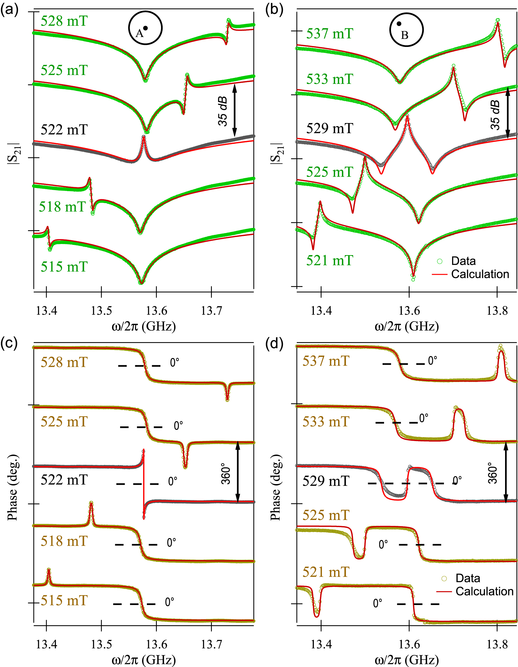
To study the line shape evolution of the transmission spectra in the strongly coupled range, five pairs of typical spectra selected from figures 3(b) and (c) (indicated by the arrows) were plotted in figures 4(a) and (b). Each spectrum of either the level attraction or the level repulsion contains two dips and one peak. For these two dips, one is the cavity-photon-like hybridized mode and the other is the magnon-like hybridized mode. At the frequency of uncoupled magnon mode, a resonant peak occurs from the coupling effect. Because of the superposition of the magnon-like hybridized mode and the resonant peak, the line shape of transmission near the magnon-like hybridized mode is in general anti-symmetric⁵ . As shown in figure 3(d), interestingly, the dispersion of resonant peak occurs at outside of the two hybridized modes. However, in the level repulsion case, the resonant peak occurs between them (figure 3(e)). The different sequences of anti-resonant dips and the resonant peak in the frequency domain result in different polarities of the transmission line shape near the magnon-like hybridized mode. From figures 4(a) and (b) we see that (1) the polarity of the asymmetry changes as it passes through the cavity mode frequency ω_A; and (2) the polarity of the line shape is opposite between the case of level attraction and level repulsion. To qualitatively explain this striking observation, we use the fact that $\kappa \gg \beta {\omega }_{A}$ to simplify the equation (7) and obtain

$$\begin{eqnarray}&&{S}_{21}(\omega )\simeq \displaystyle \frac{1}{\kappa }\left[{\rm{i}}({\omega }_{A}-\omega )+\beta {\omega }_{A}+{g}^{2}{{\rm{e}}}^{{\rm{i}}{\rm{\Phi }}}\displaystyle \frac{{\rm{i}}(\omega -{\omega }_{r})+\alpha {\omega }_{r}}{{\left(\omega -{\omega }_{r}\right)}^{2}+{\alpha }^{2}{\omega }_{r}^{2}}\right].\end{eqnarray} \tag{ 8 }$$

Zoom In Zoom Out Reset image size

The resonant feature is caused by the third term in the bracket, which includes both the symmetric and anti-symmetric line shapes [29]. The calculated result, by using either equation (7) or (8), shows that (1) the polarity of the asymmetry changes with the sign of ω_A − ω for both Φ = 0 and Φ = π and (2) the polarity of the whole line shape reverses between Φ= 0 and Φ = π. Physically, in the first case, the induced field of cavity with respect to the excitation has π phase shift with respect to the cavity anti-resonance. Consequently, the magnon mode driven by this induced field has π phase difference between these two conditions of ω < ω_A and ω > ω_A. As for the second case, depending on whether the interaction from the cavity anti-resonance to the magnon mode is the driven torque or drag torque, a π phase difference of the magnon mode would also be induced between these two situations. In both cases, the π phase difference can result in the polarity reverse of line shape near the magnon-like hybridized mode in the spectra. As shown in figures 4(a) and (b), the agreement between experimental line shape (symbols) and the calculation (solid lines) is excellent.

Correspondingly, the phase change in these five pairs of spectra has also been plotted for comparison, as shown in figures 4(c) and (d). Near the condition of ω = ω_A = ω_r, a single 2π-phase jump appears for level attraction, while for level repulsion two π-phase drops, corresponding to two hybridized anti-resonance modes, can be observed along with an additional opposite π-phase jump between them. At the condition of ω_r < ω_A, the cascaded phase of the resonant peak and the magnon-like hybridized mode merge as a peak lying on the top of the phase background (∼π/2) for level attraction and a dip for level repulsion. In contrast, at the condition of ω_r > ω_A, the cascaded phase of the magnon-like hybridized mode and the resonant peak merge as a dip lying on the bottom of the phase background (∼ −π/2) for level attraction and a peak for level repulsion.

These features can be intuitively understood by considering the relative sequences of anti-resonant dips and resonant peak at different external field, shown in figures 3(d) and (e). In the case of level attraction for instance, at the condition of ω_r < ω_A, the frequency of resonant peak is lower than the magnon-like anti-resonance. As we have mentioned in section 2.1, resonance corresponds to a π phase increase, while anti-resonance corresponds to a π phase decrease. Therefore, the cascade phase near the magnon-like hybridized mode increases first, and then decreases. Consequently, a peak occurs on the top of the phase background. Similarly, we can easily explain the phase behavior near the magnon-like hybridized mode at the condition of ω_r > ω_A. Specially, the 2π phase drop in the level attraction case at the condition of ω_r = ω_A can be explained by the coalescence of two hybridized anti-resonance modes.

As shown in figures 4(c) and (d), the experimental line shape (symbols) and the calculation (solid lines) is in excellent agreement without any adjusting parameters. Even though the magnitude and phase spectra of the microwave transmission exhibit contrasting characteristics between level attraction and level repulsion, all of them can be well reproduced using either equation (7) or (8). This confirms the validity of our model for analyzing and fitting the transmission spectra for both coherent and dissipative coupled magnon-photon systems.

To further reveal the tunability of the coupling effects in the cylindrical cavity, another experiment has been designed to observe the transition from level repulsion to level attraction. The experiment set-up is shown as the insert of figure 5(a), where the simulated rf h-field distribution clearly shows a four-fold symmetry. Therefore, by rotating the YIG sphere within the cavity a distance of 6 mm from the outer edge, the relative impact of Ampère's Law and Lenz's Law can be manipulated continuously. As a result, the coupling strength g as a function of the angular position θ for the YIG sphere should reflect such a symmetry.

Zoom In Zoom Out Reset image size

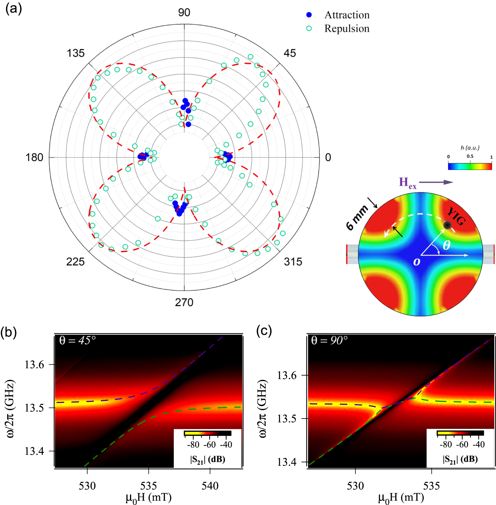
Setting θ = 45° (or an odd multiple of 45°) at an rf h-field anti-node, level repulsion occurs as shown in figure 5(b). By fitting the dispersion (dashed lines) according to equation (6), the deduced coupling strength is g/2π = 32 MHz. Rotating to θ = 90° (or an integer multiple 90°), at an rf h-field node, level attraction appears in figure 5(c) with a coupling strength of g/2π = 16 MHz.

The determined coupling strength g as a function of the angular position θ of the YIG sphere is summarized in figure 5(a) using the solid circles for level attraction and open circles for level repulsion. The dotted line follows a simple $| \sin (2\theta )|$ relation according to the linear dependence of the coherent coupling strength on the local h-field strength of the mode profile. It is clearly seen that this simple model cannot fully explain our experimental results because level attraction is beyond this model. In figure 5(a) we can find two distinct coupling regions: the level attraction region for θ near integer multiples of 90° (over a range of about ±6°) and level repulsion for θ near odd multiples of 45° (over a range of about ±39°). Experiments also indicate that the range of level attraction expands when the YIG is placed closer to the center of the circle. All these features are consistent with the results discussed based on the classical picture in [25], confirming that two competing magnon-photon coupling effects coexist in general experimental conditions. Only by minimizing the coherent coupling caused by the h-field torque, the dissipative magnon-photon coupling would reveal, allowing the observation of level attraction.