


Abstract
Results of angle-resolved electron spectroscopy of near-threshold photoionization of Ne atoms by combined femtosecond extreme ultraviolet and near infrared fields are presented. The dressed-electron spectra show an energetic distribution into so-called sidebands, being separated by the photon energy of the dressing laser. Surprisingly, for the low kinetic energy (few eV) sidebands, the photoelectron energy varies as a function of the emission angle. Such behavior has not yet been observed in sideband creation and has not been predicted in commonly used theoretical descriptions such as strong field approximation and soft photon approach. Describing the photoionization with a time-dependent Schrödinger equation allows a qualitative description of the observed effect, as well as the prediction of fine structure in the sideband distribution.
Export citation and abstract BibTeX RIS

Original content from this work may be used under the terms of the Creative Commons Attribution 3.0 licence. Any further distribution of this work must maintain attribution to the author(s) and the title of the work, journal citation and DOI.
1. Introduction
Combining extreme ultraviolet (XUV) free-electron laser (FEL) radiation with intense optical or near infrared (NIR) laser fields opens up a wide range of laser assisted photoionization experiments [1–7]. Electrons emitted by XUV photoionization during an intense multi-cycle NIR field experience the quantum nature of the dressing field and can be shifted in energy by an integer number of NIR quanta, ±ℏωL, and hence change angular momentum. In the electron spectrum, the main photoelectron line is split into a multitude of lines called sidebands [1, 3, 8]. In the quantum-mechanical picture, the appearance of sidebands is the result of the interference between electron waves emitted at different periods of the optical laser pulse [1, 2, 9]. Such experiments, therefore, provide a sound testing ground to study fundamental multiphoton processes and to investigate the validity of theoretical approaches aiming to describe these nonlinear phenomena.
The presented two-color XUV–NIR photoelectron spectra of low energy (E < 10 eV) electrons have been obtained at the FEL FLASH in Hamburg [10]. The angularly resolved spectra show a dependence, so far not described, of the kinetic energy of the electrons emitted in the sidebands as a function of the emission angle. The measured kinetic energy of sideband electrons emitted parallel to the NIR polarization (low angles) is higher as compared to electrons emitted perpendicular to the NIR polarization. At intensities of more than 2 × 10¹² W cm−2 this 'tilting' of the sidebands in the angular distribution is significantly larger than the ponderomotive potential of the NIR pulse.
To get more insight in the processes involved simulations were performed. Most reported sideband experiments so far have used photoelectron energies exceeding 15 eV that can be accurately described within the strong field approximation (SFA) approaches treating the emitted electron as a free particle interacting with the laser field without the influence of the parent ion [5, 9, 11]. For kinetic energies <15 eV more sophisticated approaches are necessary which take into account the simultaneous interaction of the electron with ionic and radiation fields. A well-established means to circumvent this problem is to solve the time-dependent Schrödinger equation (TDSE) describing the motion of the slow photoelectron in both fields [4, 12, 13]. The TDSE calculations in the present work show indeed an energy shift as a function of the emission angle, in contrast to the widely used SFA approach which predicts no angular dependence of the sideband photoelectrons. In addition, the TDSE simulation predicts that sidebands deviate from the known Gaussian energy distribution to a more and more filamented distribution leading to the splitting of each photoelectron line for intensities above 4 × 10¹² W cm−2.
We note that there is a certain similarity between near-threshold two-color XUV+NIR ionization and one-color above-threshold ionization (ATI) by a strong NIR laser field. Thus ATI calculations and experiments have observed similar effects such as the angular dependence of the ATI peak intensity [14, 15] as well as the splitting of the ATI peaks at low energy [15–19]). However, due to the highly nonlinear nature of the process, and the fact that in addition resonant multiphoton processes are involved, the ATI case is much more complex to interpret.
In the present work we explore experimentally and theoretically two-color XUV+NIR ionization of Ne atoms in the near-threshold region. The paper is organized as follows: In section 2, we give the details of the experiment to measure the angular distribution of sidebands with low kinetic energy. In section 3, we describe the calculations of the electron spectra and the angular distribution based on the numerical solution of the TDSE. In section 4, the results of the experiment are compared with the TDSE calculations and with simulations which take into account the fluctuating properties of the FEL pulses.
2. Description of experiment
2.1. Description of FEL and NIR laser parameters
The measurement was performed at the CAMP endstation [20] at the beamline BL1 of the FEL FLASH at DESY [10]. The FEL was operated at a mean photon energy of 25.2 eV (49.2 nm) with an inherent bandwidth of 0.3–0.4 eV (FWHM). The XUV pulses with an average pulse energy of ∼4 μJ (at the experiment) and a pulse duration of ∼100 fs (FWHM) were focused to a focal spot with a diameter of <50 μm. It is important to note that FLASH is operated in self-amplified spontaneous emission (SASE) mode [10]. Therefore, initial stochastic fluctuations in the electron density lead to a spiky intensity distribution of the XUV pulse rather than a well-defined Gaussian pulse. Moreover, this substructure changes substantially from pulse to pulse, as illustrated by simulated [21] SASE FEL pulses shown in figure 1. For an XUV photon energy of about 25 eV each spike has a duration of about 15–20 fs (FWHM) [22–24] leading to 4–5 spikes within the 100 fs pulse. Invoking the Fourier transform relation, the same spiky structure is present in the XUV spectral distribution, which can be measured more easily, in contrast to the temporal shape. Spectra acquired with the FLASH high-resolution spectrometer [25] showed indeed 4–5 peaks on average.
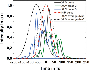
Figure 1. Illustration of the SASE XUV and NIR pulses used in the experiment. Three simulated [21] XUV SASE FEL pulses are displayed as examples (solid lines) showing the varying pulse substructure as well as the relative timing jitter compared to the NIR laser (plotted as a dashed line). As illustration for the simulation process described in section 3.2, the averaged (1000 FEL pulses) pulse shapes for best temporal overlap (corresponding to bin5) and a 60 fs temporally shifted averaged FEL pulse (corresponding to bin3) are shown as dotted lines.
Download figure:
Standard image High-resolution imageThe FEL was operated at a (single) pulse repetition rate of 10 Hz to overlap each of the XUV pulses with the NIR dressing field produced by the Ti:sapphire based pump–probe laser system at FLASH1 [26]. The 10 Hz laser system provides 70 fs (FWHM) laser pulses centered at a wavelength of 810 nm which were focused to a spot of ∼100 μm diameter. The pulse energy was ∼100 μJ to get peak intensities of ∼1 × 10¹³ W cm−2. The relative jitter between optical laser and FEL pulses was on the order of 100 fs FWHM, thus in the range of the pulse durations. In addition spatial jitter and drifts changed the intensity distributions during the measurement. Both, the FEL and NIR laser, were linearly and horizontally polarized.
2.2. Setup of the experiment
The XUV and NIR pulses were overlapped spatially and temporally in the center of the CAMP endstation [20] interacting with a collimated neon gas jet (5 mm diameter) which had a density of ∼109 atoms cm−3. The photoelectrons from the process Ne 2p6  Ne+2p5 + e− with a kinetic energy of 3.6 eV (Ne 2p binding energy: 21.6 eV) were recorded using the long (upper) side of the double-sided flat-electrode velocity map imaging (VMI) spectrometer in the CAMP endstation, equipped with an MCP/phosphor screen and a CCD camera [20]. The alignment procedures for optimizing the VMI as well as finding spatial and temporal overlap have been described in [27, 28]. The VMI collects the complete 4π solid angle of emitted electrons, measuring the projected electron angular distribution in the FEL polarization plane [29]. The extraction voltages (∼220 V cm−1) were set to cover the kinetic energy range up to 15 eV. The VMI images were recorded at 10 Hz.
Due to the spatial and temporal jitter, the recorded data fluctuated from no sidebands (no overlap) to maximum number of sidebands (best overlap). Thus, the 'effective' intensity was altered for each shot. To get sufficient statistics, more than 200 000 images were recorded in total and used for the analysis. The images were sorted according to the intensity ratio between the sidebands and the main photo line which are clearly separated in the raw images (see figure 2). Five effective intensity bins were chosen, covering the whole range between 'no sidebands' and 'maximum number of sidebands'. To reconstruct the slices of the 3D photoelectron angular distributions out of the 2D-VMI images, different methods of the inverse Abel transformation have been applied. The BASEX method [30], direct integration of the Abel integral [30] and an iterative approach [31] led to identical results. The result for bins 2–5 is shown in figure 2.
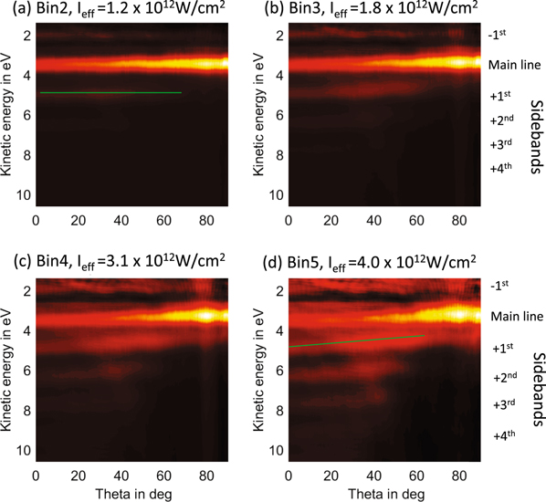
Figure 2. The measured angularly resolved photoelectron distribution from the Ne 2p ionization process in the presence of an intense NIR laser field is shown. The single-shot VMI spectra were sorted according to the relative sideband amplitude in intensity bins. Each image is averaged over more than 20.000 singe-shot images. Using the ponderomotive shift of the main line, effective intensities Ieff between 1 and 4 × 10¹² W cm−2 can be assigned to the individual bins. While for the lowest intensity only weak sideband signatures are present which show no angular energy dependence, for higher Ieff the sideband structures are increasing as well as the angular dependence of the kinetic energy in the sidebands (they are tilted). The green lines are a guide to the eye to display the tilting of the sidebands. We note that the vertical stripe at 80° is an artifact from the reconstruction.
Download figure:
Standard image High-resolution imageIn order to ensure that the experimental system was functioning correctly and to verify the data analysis codes, the well-known angular distribution for the Ne 2p photoelectron emission at ℏω ∼ 25 eV without the NIR field was analyzed. The angular distribution anisotropy parameter (β2) was determined to be −0.25 ± 0.06 which is in good agreement with the literature values of −0.23 ± 0.05 [32]. Without the NIR laser field, the Ne 2p photoelectron line as well as other reference measurements using Kr as the target gas, leading to emission lines in the range from 1 to 11 eV [33], showed no sign of tilting as a function of emission angle. Thus, we can rule out that the measured angular dependencies result from inhomogeneous fields in the VMI spectrometer.
3. Simulation of the two-color near-threshold photoionization
To compare the results of the experiments to the theoretical calculations, the ionization process was simulated for conditions close to the experimental ones. As stated earlier, the kinetic energy of the electrons after ionization is low, thus the ionization cross sections cannot be calculated within the simple SFA approach. Hence, we calculated the photoelectron spectra and their angular distributions by numerically solving the TDSE.
3.1. TDSE calculations for short coherent XUV pulses
The ionization of an atom is described within the single active electron approximation, i.e. we assume that the orbitals of all atomic electrons except the active one are frozen. This approximation is valid for moderately strong laser fields, much less than 1 a.u.; i.e. laser intensity I ≪ 1016 W cm−2, when the polarization of the core orbitals by the NIR field can be ignored. We suppose that both NIR and XUV pulses are linearly polarized and their polarization vectors are parallel. Then the ionization process is axially symmetrical with respect to the direction of polarizations which we assign as z-axis.
The motion of the active electron is described by the TDSE where the interaction of the electron with the electric fields of the two pulses is taken in the dipole approximation. The interaction of the electron with the atomic core is described by the time-independent Hartree–Slater potential [34]. The big difference in the magnitude of the XUV and the NIR fields and in the frequencies of the pulses allows one to use the first order perturbation treatment and the rotating wave approximation for the description of ionization by the XUV field. The influence of the strong NIR field is fully taken into account by the TDSE solution. By expanding the active electron wave function in spherical harmonics one gets a system of equations for partial wave functions. (For details of derivation see [13].) Note that due to the axial symmetry of the problem the projection of orbital angular momentum of the electron is conserved, not mixed by the fields, thus the calculations are performed for each projection separately.
The system of partial equations has been solved numerically. The time evolution of the partial wave functions was calculated with the split-propagation technique using the Crank–Nicolson propagator [35]. (For details see [12].) The partial amplitudes of photoionization are calculated by projecting the partial functions onto the corresponding continuum functions, eigenfunctions of the ionic Hamiltonian: (for further details see [12]). The calculated complex amplitudes determine the double differential cross section (DDCS). Examples of calculated DDCS are presented in figure 3.
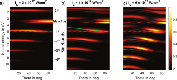
Figure 3. Angular energy distributions (DDCS) of the photoelectrons calculated with TDSE for short XUV spikes overlapped with an NIR laser at NIR peak intensities of (a) 2 × 10¹² W cm−2 and (b) 4 × 10¹² W cm−2, (c) 6 × 10¹² W cm−2. The blue dashed line indicates the expected value for the first sideband from SFA calculations which do not show any angular dependence. One can see that the kinetic energy of the sideband electrons at 90° stays constant while the kinetic energy of the electrons at small angles is shifted down for higher NIR intensities. The green line indicates the tilt of the first sideband in the case of 4 × 10¹² W cm−2.
Download figure:
Standard image High-resolution image3.2. Simulating experimental conditions
FLASH is operated in SASE mode, leading to radiation pulses consisting of a sequence of coherent spikes showing a similar temporal duration [10, 22]. In the present case, the pulse duration was on average about 100 fs (FWHM) consisting of several (on average ∼5) stochastically distributed 15–20 fs (FWHM) spikes. The spike distribution changes for each single SASE pulse. Since TDSE calculations are rather time consuming, the unpredictable nature of the SASE process prohibits extensive calculations using realistic SASE pulses. The DDCS calculated for short XUV pulses (as explained in the above section) were used as the basis to simulate the experimental results. The number of created electrons is proportional to the FEL intensity (i.e. number of XUV photons). Therefore one can add up the DDCSs calculated by solving the TDSE for defined NIR intensities and weigh them with the FEL intensity present at the corresponding NIR intensity. Since we are interested in the average DDSC for the FEL SASE case, the procedure can be simplified. Averaging the spiky single FEL pulses sufficiently (several hundreds) the resulting shape approaches a Gaussian FEL intensity distribution (see figure 1). Thus the adding and weighing DDSCs can be done by using the Gaussian XUV FEL average pulse duration.
In order to simulate the photoelectron angular distribution for all five intensity bins, we used the delay between XUV and NIR pulses. The main reason for the shot-to-shot fluctuations in the experiment (besides the changing pulse structure) is the relative timing jitter between XUV and NIR pulses. Thus, we can simulate the experimental data by introducing a delay in the averaging procedure which is 0 fs for the bin representing the highest NIR intensity (bin 5) and is larger for the other bins (e.g. 60 fs for bin 3) as is sketched in figure 1.
The actual delay values for each bin can be determined from the information of the 'effective' NIR intensity in the bin. Fortunately, the binned experimental spectra contain sufficient information to determine an 'effective' NIR intensity present during the interaction (Ieff) by using the ponderomotive shift of the main photoelectron emission line. As e.g. shown in [1, 6] the NIR field increases the ionization potential by the dynamical Stark effect, leading to a reduction of the kinetic energy of the photoelectrons by  (with the NIR intensity IL and NIR frequency ωL).
The energetic shift of the main line can be used to determine the averaged NIR intensities acting during the interaction, thus defining an 'effective' laser intensity for each bin. One has to note that the FEL spikes are significantly shorter as compared to the NIR pulse, thus during each single FEL pulse the created electrons are interacting essentially with whole range of NIR intensities (compare to figure 1).
For the highest intensity bin we get a shift of the angularly integrated main line of 0.24 eV due to the ponderomotive potential corresponding to an NIR intensity of  , see figure 2. This is, as expected, lower than the actual peak intensity of the NIR laser field due to the averaging of the laser intensities.
4. Results and discussion
4.1. Results of TDSE calculations for short XUV pulses at particular NIR peak intensities
As first step, TDSE calculations have been performed with well-defined, fully coherent XUV and distinctly longer NIR pulses (scenario A). This way we can study the interaction of a single FEL spike theoretically and determine the influence of the NIR intensity. In a second step, these single-spike photoelectron emission distributions are used to simulate the FEL pulse by averaging over several fluctuating XUV spikes (scenario B).
The parameters were chosen reasonably close to the experimental condition. The XUV photon energy was set equal to the experimental one, i.e. 25.2 eV, which yields a Ne(2p) photoelectron of 3.6 eV kinetic energy. The pulse duration was 10 fs (FWHM), which is slightly shorter as the expected SASE single spike but numerically less elaborate. Under the given conditions, calculations showed that the calculated DDCS is almost identical if the XUV pulse length and the NIR pulse length are set 1.5 times longer. The laser pulse was sufficiently longer (factor 3) than the XUV pulse to simulate the interaction with a rather well-defined NIR intensity, close to the peak intensity. The calculations were performed for an NIR intensity range from 5 × 10¹¹ to 1 × 10¹³ W cm−2. Here, we discuss the results of TDSE calculations for some representative peak intensities of 2.0, 4.0 and 6.0 × 10¹² W cm−2 as shown in figure 3 for scenario A.
In the case of near-threshold two-color photoionization two new features are evident. First, at sufficiently large intensity (figures 3(b) and (c)) the sidebands show clearly an angular dependence: the energy of the sideband is smaller at 0° than at 90°. The effect increases with increasing intensity. Interestingly, the sideband position at 90° (perpendicular to the NIR polarization) does practically not change for different intensities (see blue dashed line in figure 3), while at lower angles (close to the polarization direction) the kinetic energy shifts to smaller values. Note that this angular dependence is opposite to that observed in the experiment. The seeming contradiction is resolved when the averaging due to the SASE spikes is accounted for (see discussion in section 4.2 and figure 4 for scenario B).

Figure 4. Comparison of the experimentally measured angular distribution of the emitted photoelectrons (b), (d) and the theoretical result obtained by combining the TDSE with SASE pulses (a), (c). (a) and (b) Show the simulated and experimental data for an effective intensity of  (experimental bin 5) and (c), (d) for
  (experimental bin 3), respectively. Inset: magnified view of the first sideband. The blue crosses indicate the center of mass of the sideband indicating the angular dependence. The green line is a guide to the eye showing the 'upwards' tilting.
Download figure:
Standard image High-resolution imagePresumably, the tilting is related to the rescattering of slow electrons from the ionic core. The slow electrons driven by the strong NIR field can revisit the residual ion and after scattering they can interfere with the directly emitted ones. The interference of the rescattered wave packet, modified by the time-dependent NIR field and the emitted wave packet, can strongly modify both, the angular distribution and the energy spectrum. As shown in [36, 37] for photoionization by attosecond XUV pulses, rescattering drastically changes the electron spectra in forward and backward directions with respect to the NIR field polarization. At the same time, in the perpendicular direction the influence of rescattering is practically negligible. For fast photoelectrons this effect is negligible and the position of the sidebands is independent of the emission angle. Note that in case of ATI, the dependence of the ATI peak position on the emission angle, has been observed (e.g. [14, 15]) but has not been discussed in detail.
The second interesting feature of the sidebands in the near-threshold region is 'filamentation', that is splitting of the sidebands. Indeed, at large peak intensities (above 3 × 10¹² W cm−2) the sidebands split in two or sometime three lines (see figure 3(c)). In our calculations the splitting can be seen not only in sidebands, but also in the main line. Analogous splitting of ATI peaks is a well-known fact confirmed both experimentally [15–17] and theoretically [17–19, 38]. The first observation of a narrow fine structure of the individual ATI peaks was reported by Freeman et al [16] for subpicosecond laser pulses. It was interpreted as a resonant enhancement in the ionization process produced by ponderomotive shifts of states. An alternative explanation of the origin of the ATI peak fine structure was suggested by Eberly et al [39, 40]. In their model calculations the substructure of the ATI peaks appears because of multiphoton ionization of weakly transiently excited atomic states which are dipole-connected to the ground state.
A similar interpretation can be applied in our case of near-threshold two-color ionization. The wave packet of a slow electron created by the XUV pulse, is driven by the NIR electric field. It can be diffracted by the residual ion, thus transiently exciting Rydberg states which can lead to the fine structure of the sidebands. Such complicated dynamics which involves also interference of the undistorted wave packet and the rescattered one was analyzed by solving TDSE in [12, 36, 37] for near-threshold ionization by attosecond XUV pulses in the presence of NIR laser field. In the present calculations, the solution of the TDSE for femtosecond pulses includes the above mentioned phenomena and results in the sideband fine structure as displayed in figure 3. For the present experimental situation, the averaging over a large range of intensities washes out the filamentation effect (as seen in figure 4).
4.2. Comparison of measured and simulated photoelectron angular distributions for SASE FEL pulses
Using the averaging of the calculated DDCS, as described in section 3.2, the angularly resolved photoelectron spectra can be simulated and compared to the measurements. In figure 4 the angularly resolved photoelectron spectra are shown for two different effective NIR intensities ((a), (b)  (bin5 in figure 2) and (c), (d)
  (bin3 in figure 2)). Different features can be observed and will be discussed below.
In the experiment, the first sideband at the low kinetic energy side (−1st) has a rather constant intensity distribution as a function of the emission angle. While on the higher energy side as the order of the sidebands increases, one can see from figure 4 that the angular distribution becomes more concentrated around 0°. The higher order sidebands (3rd and higher) show essentially no contribution for emission angles exceeding 45°. These features have already been observed for photoelectron and Auger sidebands at larger electron energies [2, 3, 5] and can be easily explained within simple models of sideband formation. Considering long NIR pulses, the intensity of the sideband of the order n is proportional to  [8, 11] where Jn is the Bessel function, AL is the amplitude of the vector potential of the NIR field, ωL is its frequency, and
  is the electron wave number. In our case, the parameter
  is small. For small arguments (
 ) the Bessel function is proportional to
  , thus the intensity of the nth sideband is proportional to
  . Therefore, with increasing n the angular distribution is more and more concentrated around θ = 0.
A much more interesting observation is the dependence of the electron kinetic energies of the sidebands (on the higher energetic side of the main line) on the emission angle. Looking at the experimentally measured spectra in figures 4(b), (d), one notes, that the mean kinetic energy of the main line and the higher energetic sidebands, predominantly the +1st sideband, are shifted to lower kinetic energies at higher angles.
To compare the simulations based on SASE pulses and the experimental results in more detail, the insets in figure 4 show the enlarged +1st sideband with a (green) line indicating the observed tilt. The green line represents a slope of −0.75 eV between 0° and 90° for the experimental case and −0.35 eV for the simulation. Though the SASE simulation is based on a very crude and simplified model, the main features observed in the experiment can be reproduced. The simulation shows the tilt in the same direction as the experiment, however, the effect is less pronounced in the simulation, which can be attributed to the insufficient modeling of the (unknown) SASE fluctuations. As pointed out before, the shift in the simulations using short XUV pulses at a well-defined NIR intensity (figure 3) shows a tilt in the opposite direction.
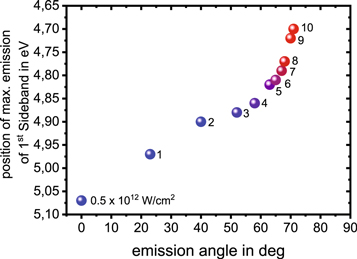
How does the averaging change the sign of the tilt and influence electrons differently at small and large angles? A closer look to the photoelectron spectral distribution for the short XUV pulses interacting with well-defined NIR intensities (figure 3) can explain the observations. The main fraction of the electrons in one sideband (particularly pronounced in the +1st one) is emitted within a rather small angular region. This effect becomes more pronounced for higher NIR intensities (compare figures 3(b) and (c)). With increasing intensity this emission maximum of the sidebands shifts to larger angles (closer to 90°) and to lower kinetic energies. Figure 5 shows the emission angle and peak kinetic energy of the emission maximum of the first sideband from the TDSE calculations as a function of NIR intensity. Thus, summing all NIR intensity contributions according to our SASE model (figure 4), we indeed get the 'upwards' tilting of the sidebands which can qualitatively explain the experimental finding.
Figure 5. Emission angle and kinetic energy of the maximum of the DDCS for the first sideband in the TDSE calculations for a single short XUV spike (see figure 3). The emission maximum is plotted for NIR intensities from  showing that the main contribution of the electron emission for the sideband is shifted to higher angles and lower energies as the NIR intensity is increased. Thus, explaining qualitatively the tilting of the experimental data. The color indicates the intensity from blue (low) to red (high intensity). The peak intensity value is printed next to the data points in units of 1012 W cm−2.
Download figure:
Standard image High-resolution image
This example emphasizes the importance of a detailed modeling of the process in particular when pulses containing a complex substructure, as in the case of SASE, are involved. Thus, averaging over pulse structure fluctuations can alter the behavior of certain effects completely. To finally reveal the sideband features near threshold, i.e. tilting and filamentation, predicted by theory, experiments using high harmonic generation or seeded FELs will be required.
5. Conclusion
Angularly resolved photoelectron spectra of neon in a two-color experiment with SASE FEL XUV pulses and NIR laser pulses were recorded. The low-energy photoelectrons (Ekin = 3.6 eV) are emitted into an intense NIR laser field leading to sideband structures. The angular distributions of the resulting sidebands show a shift towards lower kinetic energies for larger emission angles (closer to 90°). This shift is opposite to that predicted by the TDSE calculations for short XUV pulses. If the chaotic nature of the SASE FEL pulses is considered, the necessary averaging leads to an effective shift to lower energy for larger angles, explaining the experimental findings qualitatively. In addition, the TDSE calculation predicts a fine structure in the sideband angular distribution for intensities exceeding 3 × 10¹² W cm−2 for short XUV pulses, which, however, is averaged out if employing fluctuating FEL pulses. The study emphasizes the great importance of the underlying pulse parameters for the basics of nonlinear light–matter interaction, especially at SASE based FELs, which is impacting a broad variety of two-color experiments.
Acknowledgments
We want to acknowledge the work of the scientific and technical team at FLASH. We acknowledge the Max Planck Society for funding the development and the initial operation of the CAMP endstation within the Max Planck Advanced Study Group at CFEL and for providing this equipment for CAMP@FLASH. The installation of CAMP@FLASH was partially funded by the BMBF grants 05K10KT2, 05K13KT2, 05K16KT3 and 05K10KTB from FSP-302. NMK acknowledges hospitality and financial support from FS-DESY and from the theory group in cooperation with the SQS work package of European XFEL (Hamburg). The participation of the DCU group was made possible by Science Foundation Ireland grant nos. 12/IA/1742 and 16/RI/3696. PJ acknowledges support from the Swedish Research Council and the Swedish Foundation for Strategic Research. MI acknowledges funding by the Volkswagen Foundation within a Peter Paul Ewald-Fellowship. AKK acknowledges the support of the Spanish Ministerio de Economia y Competitividad (grants FIS2016-76617-P and FIS2016-76471-P).