

Abstract
Radio frequency capacitively coupled plasmas (RF CCPs) sustained in fluorocarbon gases or their mixtures with argon are widely used in plasma-enhanced etching. In this work, we conduct studies on instabilities in a capacitive CF4/Ar (1:9) plasma driven at 13.56 MHz at a pressure of 150 mTorr, by using a one-dimensional fluid/Monte-Carlo (MC) hybrid model. Fluctuations are observed in densities and fluxes of charged particles, electric field, as well as electron impact reaction rates, especially in the bulk. As the gap distance between the electrodes increases from 2.8 cm to 3.8 cm, the fluctuation amplitudes become smaller gradually and the instability period gets longer, as the driving power density ranges from 250 to 300 W m−2. The instabilities are on a time scale of 16–20 RF periods, much shorter than those millisecond periodic instabilities observed experimentally owing to attachment/detachment in electronegative plasmas. At smaller electrode gap, a positive feedback to the instability generation is induced by the enhanced bulk electric field in the highly electronegative mode, by which the electron temperature keeps strongly oscillating. Electrons at high energy are mostly consumed by ionization rather than attachment process, making the electron density increase and overshoot to a much higher value. And then, the discharge becomes weakly electronegative and the bulk electric field becomes weak gradually, resulting in the continuous decrease of the electron density as the electron temperature keeps at a much lower mean value. Until the electron density attains its minimum value again, the instability cycle is formed. The ionization of Ar metastables and dissociative attachment of CF4 are noticed to play minor roles compared with the Ar ionization and excitation at this stage in this mixture discharge. The variations of electron outflow from and negative ion inflow to the discharge center need to be taken into account in the electron density fluctuations, apart from the corresponding electron impact reaction rates. We also notice more than 20% change of the Ar+ ion flux to the powered electrode and about 16% difference in the etching rate due to the instabilities in the case of 2.8 cm gap distance, which is worthy of more attention for improvement of etching technology.
Export citation and abstract BibTeX RIS
1. Introduction
Etching and deposition are key steps in the manufacturing process of micro-electromechanical systems and very large scale integrated circuits [1–3]. Radio frequency capacitively coupled plasmas (RF CCPs) are widely used in plasma enhanced etching and deposition due to their simple geometry and large area processing structure [3–6]. Usually, much research attention is drawn to the heating mechanism [7], discharge mode [8], separate control of ion flux and energy [9], radial uniformity [10] as well as the chemistry of mixed gases [11], which are of fundamental interest in sustaining and modulating capacitive discharges, for the purpose of realizing high efficiency and quality in microelectronics production.
Generally, electronegative gases, like O2, Cl2, CF4 and SF6, are widely employed in industrial etching and deposition processing [12–15]. As the feature size gradually decreases, further understanding and subtle modulation of ion energy and flux [16–24], etching rate [25–28], neutral flux [29, 30] are important in CCPs sustained in fluorocarbon gases or their mixtures with argon and oxygen, which have been used frequently in both atomic layer etching [12, 24] and high aspect ratio etching (HARE) [16]. In order to realize flexible control of ion energy distributions (IEDs), dual frequency (DF) CCP [17] and the electrical asymmetry effect [17, 18] with the fundamental frequency and its second harmonic driving sources have received wide attention instead of traditional single frequency CCP. With the introduction of the third harmonic in Ar and Ar/CF4/O2 CCPs, phase shifts between the fundamental frequency and its harmonics are considered as valid control variables, not only for energies and their widths of IEDs, but also for the enhanced plasma density and improved uniformity [17]. And, with the requirement of allowing the injection of negative ions or high energy electrons to penetrate into etching feature and neutralize positive charge accumulation, pulse modulated DF CCPs [19], DC-RF CCPs [20], and tailored voltage waveforms [21, 22] are considered as promising candidates for HAR hole or trench etching. Besides, due to the synergistic effect of ions and neutrals on the etching profiles, radicals' generation from gas dissociation in the plasma bulk and their fluxes, as well as the flux ratio between them to ions, deserves much attention for the improvement of selectivity and etching rate [27, 29]. On the other hand, different from electropositive gases, electronegative fluorocarbon discharges exhibit higher electron heating in the bulk due to a high voltage drop across the plasma bulk, resulting in high ionization and dissociation rate, which would affect the negative dc bias and separate control of ion properties [23].
The working gases in etching are usually complex mixtures of reactive and electronegative gases like fluorocarbon and oxygen, as well as the typical electropositive gas argon. The addition of negative ions and metastable neutrals affects the discharge properties, not only on a timescale less than a microsecond within one RF period, but also showing some unstable behaviors like periodic fluctuations on larger timescales [29–31, 32–34]. Katsch et al [31] observed fluctuations of the plasma potential and light emission in an RF excited discharge in oxygen, owing to an attachment induced ionization instability in which the formation and loss of negative oxygen ions by electron attachment and metastable molecules are considered to be the main reasons. In addition, in low pressure SF6 and Ar/SF6 inductive discharges, oscillations on the order of millisecond in the experiment and global simulations were observed in charged particle densities, electron temperature and plasma potential, suggesting instabilities at a transition region between capacitive and inductive modes in a strongly electronegative plasma [32]. Furthermore, a two-dimensional simulation was conducted to discuss time and space resolved variations of the inductive-capacitive transition instability in a Cl2 electronegative discharge [33]. Millisecond periodic instabilities were also observed in a planar-coil inductive discharge sustained in pure CF4 gas [34], in which they noticed that the radical density fluctuations (such as CF, CF2) are significant at frequencies of about 1 kHz, resulting from chemical reactions. Moreover, instabilities in low pressure inductive chlorine discharges were investigated on the basis of global simulations [35], in which the role of excited neutrals in detachment of negative ions is evaluated. Meanwhile, instabilities in a capacitively coupled oxygen plasma were also experimentally reported [36, 37], in which the electron attachment and detachment processes were considered to be responsible for the instabilities, suggesting the important role of electron heating and metastable molecules in electronegative discharge understanding. Additionally, instability phenomena on the order of microseconds in capacitive electropositive Ar plasmas [38] were observed and interpreted by an inseparable relationship with the external matching of the power source, with the increase in resistance and capacitance of the discharge when the plasma ignites.
From the above experiment and simulation studies, instabilities are widely observed in various plasmas, but the reasons for their generation still remain unclear and have to be studied in more detail. In this work, we noticed and tried to explain an instability observed in a capacitive CF4/Ar discharge, by using a one dimensional fluid/Monte-Carlo (MC) hybrid model. Compared with global and pure fluid models such as those used in references [32, 33, 35], the hybrid model allows us to treat electrons kinetically and consider spatial transport of more ions and neutrals, which is more likely to ensure accuracy and is beneficial to for the understanding of the observed instabilities. The article structure is as follows: a description of the computational model is presented in section 2. Section 3 discusses the simulation results, and finally, conclusions are given in section 4.
2. Model description
The computational research reported in this article is carried out by using a one-dimensional fluid model coupled with the Poisson's equation and the electron MC method. In the fluid model, the continuity equation is used for electrons and ions, as shown in equation (1),

where nj
, Γj
and  are density, flux and the source term of species j, and kαj
represents the rate coefficient for collisions between particle α and j. And since the electron mass is small and its inertial term can be neglected, the electron drift-diffusion approximation is adopted as
are density, flux and the source term of species j, and kαj
represents the rate coefficient for collisions between particle α and j. And since the electron mass is small and its inertial term can be neglected, the electron drift-diffusion approximation is adopted as

where e, me
, Te
, and E are the elementary charge, electron mass and temperature, and the electric field. The electron–neutral collision frequency is expressed by  , where nAr and
  are the densities of the background gas Ar and CF4, and kel−Ar and
  obtained from the electron MC model are the momentum transfer coefficients between electrons and the background gas.
The ion temperature is considered to be room temperature (about 300 K) for the cold fluid assumption, while their transport could be described by the momentum balance equation, as follows,

where mi
, ui
, Ze and p represent the ion mass, velocity, as well as the ion charge and pressure in a sequence. The two items on the left-hand side are the acceleration term and advection flux term. And on the right-hand side, we see the pressure gradient, drift flux term due to the electric field force, and the source term due to the friction force. Here,  , where νi,n
is the ion–neutral momentum transfer frequency, mn
is the neutral mass.
, where νi,n
is the ion–neutral momentum transfer frequency, mn
is the neutral mass.
The combination of the neutral continuity and diffusion equation yields equation (4), which can be used to describe the neutral density and transport, as

where Dn
and Sn
are the diffusion coefficient and source term. Here, based on the Blanc law, the diffusion coefficient Dn
of neutral species n is determined by the corresponding coefficients in the background gas Ar and CF4. The detailed expression of Dn
can be found in reference [39], in which the binary collision diameters (σi
) and potential energies (ɛi
/kb
) are given in table 1. Additionally, the electric potential Φ and electric field  are obtained through Poisson's equation.
Table 1. Lennard-Jones parameters and viscosity coefficient of neutral particles.
| Neutrals | σi (Å) [43] | ɛi /kb (K) [43] | ηi [44] |
|---|---|---|---|
| Ar* | 3.542 | 93.3 | 0.8 |
| CF3 | 4.32 | 121 | 0.017 |
| CF2 | 3.98 | 108 | 0.02 |
| CF | 3.3 | 125 | 0.036 |
| F | 2.970 | 112.6 | 0.02 |
| F2 | 3.357 | 121.6 | 0.02 (Assumed) |
In addition, boundary conditions are needed to solve the above differential equations. The electron density is assumed to follow the Boltzmann distribution  at the boundary. The electron fluxes at the electrodes are set as
  , where
  is the electron thermal velocity. And Θ represents the reflection coefficient of electrons on the electrode, which is set at 0.25 in agreement with previous particle-in-cell and fluid simulations [40, 41] that yielded good agreement with experiments. Here, the secondary electron emission coefficient γ which is dependent on the ion kinetic energy at the electrodes is calculated according to reference [42]. The heat conduction term is ignored in the electron energy flux boundary, while the convection term at the electrodes is set as
  . For positive ions, the densities and fluxes at the electrodes are considered to be continuous, and, for negative ions, their densities and fluxes are set to zero. Considering neutrals will attach to the electrodes, the neutral flux at the electrodes is set as
  , where Γn
, uth,n
and ηi
represent the neutral flux, thermal velocity and viscosity coefficient as shown in table 1. The electric potentials at the powered electrode (x = 0) and the grounded electrode (x = d) satisfy
, where Γn
, uth,n
and ηi
represent the neutral flux, thermal velocity and viscosity coefficient as shown in table 1. The electric potentials at the powered electrode (x = 0) and the grounded electrode (x = d) satisfy  and V(t)|x=d
= 0 respectively.
and V(t)|x=d
= 0 respectively.
The time and space resolved electron energy and its distribution, as well as the reaction rate coefficients are obtained based on the electron MC method [49, 50]. More details of the MC computation have been introduced in our previous work [49] in which non-equilibrium dynamics of electrons had to be accounted for in hybrid investigations of pulsed RF discharge, like what we have done in reference [49]. 30 000 pseudoparticles adopted to represent electrons are distributed in the whole discharge region and the time and space resolved electric field obtained from the fluid model is introduced to advance the velocities and locations of the pseudoparticles. The electric field is updated each RF cycle to address the time varying behavior exactly, which is surely important in this instability analysis. The velocities and positions of electrons are also affected by collisions with neutrals. The electron dynamic variables are collected at each time step and the electron energy distribution function (EEDF) is determined statistically after each RF cycle. And then, the time and space resolved reaction rate coefficient, electron temperature, and electron transport coefficients are calculated on the basis of the newly updated EEDF and transmitted to the fluid simulation. The fluid model and the electron MC method alternately run-up to more than 30 000 RF cycles to obtain the final steady state solution of the fluid model, especially considering the slow temporal evolution of negative ions.
Totally, 9 charged particles (electron, Ar+, CF3 +, CF2 +, CF+, F+, C+, F−, CF3 −) and 6 neutrals (Ar*, CF3, CF2, CF, F, F2) are taken into consideration and 51 gas phase reactions are involved in this work. The electron-impact reactions, including elastic, ionization, excitation, dissociative attachment collisions, are listed in table 2, while the ion–ion, ion–neutral, and neutral–neutral reactions have been shown in table 3, according to references [45–48], in which the corresponding electron cross-sections or rate coefficients are referred. In this work, all the rate coefficients of the electron impact reactions are obtained by the integral [49, 50] on the basis of the time and space resolved EEDF. Under the same discharge conditions, our calculation results including the magnitude of particle densities are validated with those in references [51, 52].
Table 2. Electron-impact reactions considered in the model. By means of the cross-sections in the references, the corresponding rate coefficients are obtained on the basis of the MC method
| # | Reaction | Threshold (eV) | Reference |
|---|---|---|---|
| R1 | e− + Ar → Ar+ + 2e− | 15.6 | [45] |
| R2 | e− + Ar → Ar* + e− | 11.56 | [45] |
| R3 | e− + Ar → Ar + e− | 0 | [46] |
| R4 | e− + Ar* → Ar+ + 2e− | 4.14 | [45] |
| R5 | e− + Ar* → Ar + e− | −11.56 | [45] |
| R6 | e− + CF4 → CF4 + e− | 0 | [47] |
| R7 | e− + CF4 → CF3 + + F + 2e− | 16 | [47] |
| R8 | e− + CF4 → CF2 + + 2F + 2e− | 21 | [47] |
| R9 | e− + CF4 → CF+ + F2 + F + 2e− | 26 | [47] |
| R10 | e− + CF4 → F+ + CF3 + 2e− | 34 | [47] |
| R11 | e− + CF4 → C+ + CF2 + F + 2e− | 34 | [47] |
| R12 | e− + CF4 → CF3 + F + e− | 12 | [47] |
| R13 | e− + CF4 → CF2 + 2F + e− | 17 | [47] |
| R14 | e− + CF4 → CF + F2 + F + e− | 18 | [47] |
| R15 | e− + CF4 → F− + CF3 | 0 | [47] |
| R16 | e− + CF4 → F + CF3 − | 0 | [47] |
| R17 | e− + CF4 → CF4(v1) + e− | 0.108 | [47] |
| R18 | e− + CF4 → CF4(v3) + e− | 0.168 | [47] |
| R19 | e− + CF4 → CF4(v4) + e− | 0.077 | [47] |
| R20 | e− + CF4 → CF4 * + e− | 7.54 | [47] |
aNote: CF4(v1), CF4(v3), CF4(v4) denote the products of CF4 vibrational excitation reactions into the respective vibrationally excited state. CF4 * indicates the product of CF4 electronic excitation reaction.
Table 3. Ion–ion, ion–neutral and neutral–neutral reactions and their corresponding rate coefficients.
| # | Reaction | Rate coefficient (cm3 s−1) | Reference |
|---|---|---|---|
| R21 | F− + Ar+ → Ar + F | 2.0 × 10⁻⁷ | [48] |
| R22 | F− + CF3 + → CF3 + F | 8.70 × 10⁻⁸ | [48] |
| R23 | F− + CF3 + → CF2 + F2 | 2.0 × 10⁻⁷ | [46] |
| R24 | F− + CF2 + → CF2 + F | 9.1 × 10⁻⁸ | [48] |
| R25 | F− + CF+ → CF + F | 9.80 × 10⁻⁸ | [48] |
| R26 | F− + F+ → 2F | 3.1 × 10⁻⁷ | [48] |
| R27 | CF3 − + Ar+ → CF3 + Ar | 2.0 × 10⁻⁷ | [48] |
| R28 | CF3 − + CF3 + → 2CF3 | 1.5 × 10⁻⁷ | [48] |
| R29 | CF3 − + CF2 + → CF3 + CF2 | 5.0 × 10⁻⁷ | [46] |
| R30 | CF3 − + CF+ → CF + CF3 | 2.0 × 10⁻⁷ | [48] |
| R31 | CF3 − + F+ → CF3 + F | 2.5 × 10⁻⁷ | [48] |
| R32 | CF3 + + e− → CF2 + F | 8.0 × 10⁻⁸ × Te−0.5 | [48] |
| R33 | F− + CF3 → CF4 + e− | 4.0 × 10⁻¹⁰ | [48] |
| R34 | F− + CF2 → CF3 + e− | 3.0 × 10⁻¹⁰ | [48] |
| R35 | F− + CF → CF2 + e− | 2.0 × 10⁻¹⁰ | [48] |
| R36 | F− + F → F2 + e− | 1.0 × 10⁻¹⁰ | [48] |
| R37 | CF3 − + F → CF3 + F− | 5.0 × 10⁻⁸ | [48] |
| R38 | CF2 + + CF2 → CF2 + CF2 + | 1.0 × 10⁻⁹ | [48] |
| R39 | F+ + F → F + F+ | 1.0 × 10⁻⁹ | [48] |
| R40 | CF+ + CF2 → CF + CF2 + | 1.0 × 10⁻⁹ | [48] |
| R41 | CF3 + + CF3 → CF3 + CF3 + | 1.0 × 10⁻⁹ | [48] |
| R42 | CF+ + CF3 → CF + CF3 + | 1.71 × 10⁻⁹ | [48] |
| R43 | F+ + CF3 → F2 + CF2 + | 2.9 × 10⁻⁹ | [48] |
| R44 | Ar* + CF3 → CF2 + F + Ar | 6.0 × 10⁻¹¹ | [48] |
| R45 | Ar* + CF2 → CF + F + Ar | 6.0 × 10⁻¹¹ | [48] |
| R46 | CF+ + CF → CF+ + CF | 1.0 × 10⁻⁹ | [48] |
| R47 | F + CF3 → CF4 | 2.0 × 10⁻¹¹ | [48] |
| R48 | F + CF2 → CF3 | 1.8 × 10⁻¹³ | [48] |
| R49 | F + CF → CF2 | 9.96 × 10⁻¹¹ | [48] |
| R50 | F2 + CF3 → CF4 + F | 1.9 × 10⁻¹⁴ | [48] |
| R51 | F2 + CF2 → CF3 + F | 8.3 × 10⁻¹⁴ | [48] |
3. Results and discussion
Using the typical radio frequency of 13.56 MHz in this simulation, we investigate a capacitive discharge sustained in CF4/Ar (1:9) at the pressure of 150 mTorr, with the gap distance between the electrodes at 2.8 cm for the base case scenario and the RF voltage amplitude V0 at 95.8 V, at which the deposited power density ranges from 250 to 300 W m−2, as a consequence of the observed instability. Figure 1 shows the spatio-temporal density distributions of electron, Ar+, F− and Ar*, as the main particles in this discharge. Apart from the Ar* density, the densities of electrons, Ar+ and F− all show periodic fluctuations in the bulk, at the period of about 16 RF periods (1.172 μs). To explore the electrodynamics of this instability, times of T1 to T6 are indicated by purple dashed lines for detailed discussion in the following. For instance, at time T2 in the figure, when the electron density attains its minimum value, the F− density achieves its maximum peak value in the discharge center. That is, the change trends of electron and F− densities are opposite, and the electronegativity (n−/ne
) in the bulk at time T2 becomes larger. Also at T2, the Ar+ density exhibits its lower peak value in the center, suggesting insufficient ionization. On the contrary, at time T5, we observe a maximum peak value of the Ar+ density, but a relatively lower F− density, indicating that the ionization has recovered and the electronegativity increases a lot after 8 RF periods. Within nearly 32 RF periods, the oscillations in the center are regular in time and amplitude. It is also easy to notice that, in this typical electronegative discharge, the electron density peaks located near the sheath region also show periodic fluctuations, as the ionization and electronegativity become strong or weak. From our results, the power density ![$P=\frac{1}{{T}_{\mathrm{R}\mathrm{F}}}{\int }_{0}^{{T}_{\mathrm{R}\mathrm{F}}}[V\left(t\right)J\left(t\right)]{\vert }_{x=0}\mathrm{d}t$](https://content.cld.iop.org/journals/0963-0252/31/2/025006/revision2/psstac47e4ieqn13.gif) changes between 250–300 W m−2 with the discharge fluctuations, where J(t) is the sum of the conduction and displacement current densities. However, this time varying instability is hardly noticed as the gap distance between the two electrodes increases to 4 cm and the voltage amplitude is set at V0 = 84.4 V, with the other discharge parameters unchanged, at which the power density dissipated in the discharge is about 280 W m−2.
changes between 250–300 W m−2 with the discharge fluctuations, where J(t) is the sum of the conduction and displacement current densities. However, this time varying instability is hardly noticed as the gap distance between the two electrodes increases to 4 cm and the voltage amplitude is set at V0 = 84.4 V, with the other discharge parameters unchanged, at which the power density dissipated in the discharge is about 280 W m−2.

Figure 1. Spatio-temporal density distributions of (a) electron, (b) Ar+, (c) F− and (d) Ar*. Times (purple dashed lines) of T1, T2, T3, T4, T5 and T6 are set to explore the periodic instabilities. Discharge conditions: gas mixture of CF4/Ar (1/9) at 150 mTorr with a gap separation of 2.8 cm, sustained by a 13.56 MHz, 95.8 V source supply.
Download figure:
Standard image High-resolution imageFor further understanding, we show in figure 2 the time evolution of the electron density and temperature, electric field as well as the electronegativity in the discharge center. The black dashed line in figure 2(b) represents the RF period averaged electron temperature also in the center. As we expect, they all show periodic fluctuations regularly. The electron density oscillates between 0.213 × 109 cm−3 and 0.535 × 109 cm−3 so the change in electron density is about 151.2%. The electronegativity attains its maximum at about 38 with the lowest electron density at time T2, while the drift electric field in the bulk becomes much enhanced to maintain the discharge in the presence of a lack of electrons as conductive particles. During the time interval from T1 to T3, when the electric field is enhanced and remains at relatively high values, the electron temperature rises significantly and oscillates at higher amplitudes. And even when the electric field becomes weaker after T3, the electron temperature still keeps oscillating strongly and remains at a higher averaged value until time T4, leading to a further increase of the electron density. So from T2 to T4, the electron density increases significantly, with higher electron energy owing to the heating from the bulk electric field. Until time T5, the electron density stops increasing finally and attains its maximum value in the center. Meanwhile, with the decrease of the electronegativity to the minimum value of about 15, the bulk electric field and the oscillation of the electron temperature then become much weaker. Figure 3 shows the spatio-temporal evolution of the electric field and electron heating rate (−eΓe E) at different times, respectively. It is evident to see that, the first two rows, which correspond to the cases with stronger electronegativity at T1, T2 and T3, show synergistic effects from both α mode and DA mode [8], with evident drift and ambipolar fields in the bulk, and evident electron heating from both oscillating sheath edge and bulk field, though the electron acceleration by the bulk field does not dominate, compared with that in pure and highly electronegativity CF4 discharges. But in the other two rows at times T4, T5 and T6, with the weakening of the bulk electric field, electrons are predominantly heated by the oscillating sheath, but the bulk field heating can still be observed.
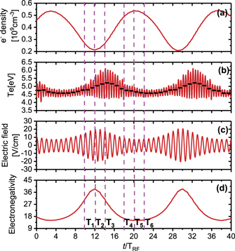
Figure 2. Time evolutions of (a) electron density, (b) electron temperature, (c) electric field and (d) electronegativity (n−/ne ) in the discharge center. Times (purple dashed lines) denoted and the discharge conditions are the same as those in figure 1.
Download figure:
Standard image High-resolution image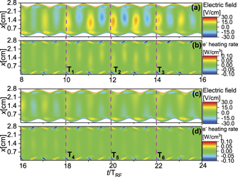
Figure 3. Spatio-temporal evolutions of the electric field and electron heating rate at time T1 to T3 in (a) and (b), and at time T4 to T6 in (c) and (d). The discharge conditions are the same as those in figure 1.
Download figure:
Standard image High-resolution imageUsually in electropositive plasmas, instabilities can hardly occur, since an initial electron density increase would lead to the decrease of the mean electron temperature and then weakened ionization which will result in the electron density decrease. From previous investigation [37, 53] in electronegative discharges, the decreasing electron temperature may cause the electron density to increase, if the attachment rate drops more quickly compared with the ionization rate, and then an instability appears. So, the fluctuating electron density and temperature are usually considered as the main variables for instability analysis. From figure 2, it is easy to observe that the change of the electric field could keep pace with those of the electron density and electronegativity, due to their close relationship coupled by Poisson's equation. Thus, they could achieve their extreme values meanwhile, at times of T2 and T5. However, a time delay can be observed between the times of the extreme values of the electric field and mean electron temperature, since it takes time for electrons to gain energy from the bulk field acceleration. From the figure, electrons may obtain more energy from the enhanced drift electric field from time T1, and keep this heating process until time T4, at which the bulk field oscillates less already. So, from T2 to T4 during the main time window of the electron density increase, the relatively higher electron temperature may lead to more electron production and cause the electron density to overshoot to a much higher value, resulting in an unstable discharge. Meanwhile, the formation of negative ions is reduced, since the cross sections for attachments are much lower at high electron energy. As a result, the electronegativity becomes much lower, as well as the bulk electric field. And then, without enhanced heating from the bulk field, electrons lose their energy gradually and it also takes time. While the electron density declines from T5, the electron temperature oscillates less and keeps a much lower mean value, leading to insufficient ionization but increasing attachment, and a much lower bulk electron density. And then, with the bulk field enhanced again, another instable cycle starts. From our results, it seems that the phase lag at which the electron temperature responds to the strong bulk field, makes the situations occur, such as both the electron density and temperature increase, or the density still decreases with smaller electron temperature, resulting in a positive feedback to the formation of the instabilities.
In order to investigate further the underlying mechanism of the instability phenomena, the source terms of the main electron impact reactions will be discussed for the corresponding analysis. First, the cross sections of the main electron impact reactions, like Ar ionization (R1), Ar excitation (R2), Ar* ionization (R4), CF4 ionization for CF3 + (R7) and CF4 dissociative attachment to form F− (R15) and CF3 − (R16), are shown in figure 4, in which we can see that the energy thresholds of Ar* ionization and CF4 dissociative attachment are much lower than those of other reactions. Figure 5 shows the spatio-temporal evolutions of the Ar ionization rate, Ar excitation rate, Ar* ionization rate, CF4 dissociative attachment rate for F−, as well as the mean electron energy. The corresponding purple dashed lines indicate the different times. As we expect, they all show periodic fluctuations regularly as well. These reactions are selected because Ar ionization and Ar excitation represent reactions impacted by higher energy electrons, while Ar* ionization and dissociative attachment reactions are those lower energy electrons tend to be involved in. In this work, all the other ionization rate distributions, such as those of CF4 ionization for generation of CF3 +, CF2 +, CF+, present almost the same evolution pictures as that in figure 5(a), but the Ar ionization rate exceeds the others by at least one order of magnitude. Besides, the dissociative attachment rate for F− generation in figure 5(d) is almost one order of magnitude higher than the rate that produces CF3 −. From figures 5(a) and (b), we can see that as the electron density becomes low enough, almost from T1, the ionization and excitation rates become more noticeable in the bulk center and get stronger near the sheath edge. Due to the high electronegativity in the bulk and the large electron density gradients near the sheath region, strong drift and ambipolar electric fields accelerate electrons from one sheath expansion to the opposite sheath collapse. Thus, the energy of electrons is increasing and becomes higher than the energy thresholds, to ionize or excite neutrals. Although the electron density begins to increase and the electric field becomes weaker in the discharge center from time T2, the Ar ionization and excitation rates are still enhanced, leading to the continuous increase of the electron density, since the mean electron energy in figure 5(e) remains at higher values until time T4. Thus, during the time from T2 to T4, the electron density in the bulk increases significantly, as discussed earlier. It can also be noticed that, although a higher rate of Ar excitation is always present near the sheath collapse (similar to Ar ionization, see figures 5(a) and (b)), the Ar* density profile tends to be relatively uniform in the bulk and does not show peaks near the sheath region, as shown in figure 1(d). Actually, the spatial profile of the Ar* density does not agree with that of the source rate, as diffusion is strong and leads to a flattening of the density profile. It was found both in PIC/MCC and fluid simulations [54, 55] that the Ar* density axial profile is center high or constant in the plasma bulk as the pressure is relatively low and similar to the pressure regime studied in this work. Only at higher pressure, peaks in the Ar* density profile near the sheath are observed. In our simulation, it is found that higher Ar excitation rates near the sheaths are efficiently attenuated by diffusion at the pressure of 150 mTorr, resulting in a relatively uniform distribution of the Ar* density in the bulk.
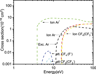
Figure 4. Cross sections of Ar ionization (red), Ar excitation (black), Ar* ionization (green), CF4 ionization for CF3 + (yellow) and CF4 dissociative attachment for F− (blue) and CF3 − (cyan).
Download figure:
Standard image High-resolution image
Figure 5. Spatio-temporal evolutions of (a) Ar ionization rate, (b) Ar excitation rate (c) Ar* ionization rate (d) CF4 dissociative attachment rate (generate F−), (e) electron temperature. Times (purple dashed lines) denoted and the discharge conditions are the same as those in figure 1.
Download figure:
Standard image High-resolution imageDuring the time from T4 to T6, with the weakening of the bulk electric field, more low energy electrons gather in the bulk, leading to the gradually faded Ar ionization and excitation in figures 5(a) and (b), and inducing more Ar* ionization and CF4 dissociative attachment to form F− in figures 5(c) and (d). The Ar* ionization only occurs in the bulk where most of the Ar* particles are located, as shown in figure 1(d). This Ar* ionization is limited but could still contribute somewhat to the electron generation during this low electronegativity time and make the electron density even higher, resulting in further instability. Though, from figure 1(d), oscillations could hardly be noticed in the Ar* density, the excitation rate for Ar* as a source term and the ionization rate of Ar* as a loss term also show periodic variations in figures 5(b) and (c). From our simulation results, the diffusion term of Ar* and the Ar excitation rate as the main terms contribute to the temporal change of the Ar* density in a similar way, leading to not only axially uniform but also temporally constant distributions of the Ar* density in the bulk. And, the CF4 dissociative attachment to form F− in figure 5(d) also shows fluctuations not just in the bulk but near the sheath region as well, where the electron density is high in electronegative discharges.
In addition, the ion dynamics is worth exploring in an unstable plasma because of the relevance of ions to etching applications. The spatio-temporal distributions of Ar+ and F− flux are shown in figure 6. Apart from the Ar+ flux in the sheath region which is much higher and not shown here, both the positive and negative ion fluxes are given and show periodic increases and decreases in the bulk region. From our simulation, compared with the other terms, the electric field term is surely the most important one to determine the ion flux in the momentum balance equation in equation (3), and the drift electric field is the dominant component in the bulk field. We show the RF period averaged electric field in the bulk that ions can respond to, for different times in figure 7, with the insert small figure for the whole discharge region. In both of the two figures, two more times, T0 and T7 are included for further understanding. From figure 7, the bulk electric field at some times shows a tiny spatial asymmetry due to the unsteady discharge state. But for the whole unstable period of about 16 RF cycles, the averaged electric field is definitely spatially symmetrical. It is easy to notice that, at time T0, the negative ion fluxes to the bulk achieve their maximum values especially near the center. So do the positive ion fluxes to the electrodes. The averaged drift electric field in the bulk is close to zero at this time, except the ambipolar field near the sheath region. Due to the relatively high electronegativity from T1 to T3, the averaged bulk electric field increases significantly, being positive and negative in the lower and upper half regions, respectively. With the action from the growing electric field force, the F− flux to the center and the Ar+ flux to the electrodes become weaker gradually. And then, from T3 to T4, the F− flux remains at a lower level along the sheath edge. During this time, electrons are heated significantly in the bulk by the drift electric field and the electron temperature in the center oscillates more strongly. Meanwhile, almost all the electron impact reactions, like ionization, excitation and attachment, become more active. From T4 to T6 when the discharge is relatively weakly electronegative, the averaged bulk electric field is negative in the lower half region and positive in the upper half region of the bulk, and makes the F− flux increase gradually again from the sheath region to the bulk center. On the contrary, Ar+ ions are accelerated from the bulk to the electrodes. Until T7, both of the ion fluxes achieve their maximum values again near the center. Meanwhile, the averaged bulk electric field returns to almost zero and the rates of almost all the electron impact reactions get close to relatively lower values.

Figure 6. Spatio-temporal distribution of (a) Ar+ flux, and (b) F− flux. Two additional times are set as control groups to explore the ion dynamics. The discharge conditions are the same as figure 1.
Download figure:
Standard image High-resolution image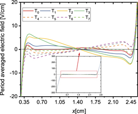
Figure 7. RF period averaged and axially resolved electric field at different times.
Download figure:
Standard image High-resolution imageFigure 8 shows the main source terms in the electron continuity equation in equation (1), including the Ar ionization rate (red bar), Ar* ionization rate (blue bar), CF4 ionization rate (CF3
+, purple bar), as well as terms of  (green bar) and
  (gray bar) on the left hand of equation (1), to present the electron dynamics in the center of this unstable discharge. We do not show the CF4 dissociative attachment rates for F− and CF3
− in this figure since they are almost 2–3 orders of magnitude smaller. All the terms in this figure have been averaged over one RF period. Firstly, from this figure, the Ar ionization rate (red bar) is the main source of electron generation, attaining its higher values at T3 and T4, as also discussed in figure 5(a). The time rate of the electron density (green bar) is mostly determined by the Ar ionization rate (red bar) and the divergence of the electron flux
(gray bar) on the left hand of equation (1), to present the electron dynamics in the center of this unstable discharge. We do not show the CF4 dissociative attachment rates for F− and CF3
− in this figure since they are almost 2–3 orders of magnitude smaller. All the terms in this figure have been averaged over one RF period. Firstly, from this figure, the Ar ionization rate (red bar) is the main source of electron generation, attaining its higher values at T3 and T4, as also discussed in figure 5(a). The time rate of the electron density (green bar) is mostly determined by the Ar ionization rate (red bar) and the divergence of the electron flux  (gray bar). At time T1, a relatively high
  means lots of electrons are expelled out of the center as a higher negative ion flux enters into the center at this time as shown in figure 6. Thus, with lower ionization rate and much higher loss by outflux, the electron density in the center still keeps decreasing. Until time T2, at which the increasing total source rates might compensate the decreasing leaving electron flux from the center, the electron density stops decreasing and attains its minimum value. And then, from T3 to T4, the continuous increase of the electron density is mostly contributed by the enhanced ionization rates induced by heated electrons, while much less electrons and negative ions are exiting or entering the center. So, during this time stage, the enhanced electron generation and less outflux of electrons make the electron density in the center increase a lot and even overshoot to a much higher value about 0.535 × 109 cm−3. At time T5, as more electrons are pushed out of the center (gray bar) and the electron source rate does not decrease too much, the time rate of the electron density becomes small and the maximum electron density is obtained. And then, with the continuous decrease of the electron source rate and the abrupt increase of the electron flux out of the center, as shown at time T6 in figure 8, the electron density at the center begins to decline again. Thus, from this figure, to make a fundamental understanding of the electron density oscillation, both the electron source term and the divergence of the electron flux are the main factors need to be considered.
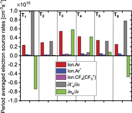
Figure 8. RF period averaged rates of Ar ionization (red bar), Ar* ionization (blue bar), CF4 ionization (CF3
+, purple bar), as well as  (gray bar) and
  (green bar) in the discharge center at the six times. The discharge conditions are the same as figure 1.
Download figure:
Standard image High-resolution imageAn overview about fluctuations of the densities of electron, Ar+ and F−, as well as the electronegativity, mean electron temperature in the discharge center, and the corresponding power density, voltage amplitude and instability period is given in table 4, at the same discharge pressure and driving frequency but the electrode gap variation from 2.8 cm to 3.8 cm. In order to compare and analyze easily, we fix the deposited power density range from 250 to 300 W m−2 with the discharge unstable fluctuations, and obtain the corresponding voltage amplitudes V0 based on lots of iteration processes in this hybrid simulation. In the case of the smallest gap distance at 2.8 cm, the electron density increases by about 151.2% and the electron temperature decreases by about 13.9%, as the discharge mode changes from a strongly to a weakly electronegative mode with the electronegativity ranging from 38.4 to 15.0. However, the positive and negative ion densities fluctuate no more than 2.2%. With the extension of the discharge space, the fluctuation amplitudes of all the main discharge variables are getting smaller gradually, and the instability period becomes longer till unnoticeable as shown in the table. As the discharge gap distance is at 3.8 cm, only weak instabilities can be observed with the fluctuations of densities only within 1.2%. Usually, there is a general decrease of electron temperature with the increase of the gap distance, as a consequence of the particle balance. For this instability, a high electron temperature is needed in the bulk, which is harder to get for larger gaps. Thus, the instability in this simulation tends to occur in plasmas with smaller electrode gap driven by almost the same power.
Table 4. Fluctuations of the discharge variables for different gap distance
| # | 2.8 cm | 3.3 cm | 3.5 cm | 3.8 cm |
|---|---|---|---|---|
| ne [109 cm−3] | 0.213–0.535 | 0.271–0.532 | 0.344–0.467 | 0.414–0.419 |
| (151.2%) | (96.3%) | (35.8%) | (1.2%) | |
 [109 cm−3] [109 cm−3] | 7.802–7.966 | 8.044–8.178 | 8.092–8.157 | 8.196–8.202 |
| (2.1%) | (1.7%) | (0.8%) | (0.07%) | |
 [109 cm−3] [109 cm−3] | 6.849–7.002 | 7.034–7.156 | 7.067–7.124 | 7.147–7.149 |
| (2.2%) | (1.7%) | (0.08%) | (0.02%) | |
| α (n−/ne ) | 15.0–38.4 | 15.4–30.8 | 17.6–24.3 | 19.8–20.2 |
| (156.7%) | (100.4%) | (37.7%) | (2.0%) | |
| Te (eV) | 4.58–5.21 | 4.57–5.05 | 4.71–4.84 | 4.69–4.74 |
| (13.9%) | (10.5%) | (2.8%) | (1.0%) | |
| P (W m−2) | 254–302 | 263–300 | 268–294 | 273–284 |
| (18.7%) | (14.3%) | (9.8%) | (4.1%) | |
| V0 (V) | 95.8 | 90.6 | 89.7 | 86.7 |
| Instability period (μs) | 1.172 | 1.475 | 1.549 | — |
In the case of 2.8 cm, in which the drift electric field in the bulk is much higher in the strongly electronegative mode, fewer electrons are accelerated significantly and get enough energy to bring strong ionization into play, which would make the electron density increase a lot. The mean electron energy in the center can stay at a high level for a relatively long time, making the electron density keep increasing and overshoot to a high value. And then, the electron temperature decreases a lot, since too many electrons have to share the limited electric power deposited. Since CF4/Ar gas is also a typical electronegative gas in which the electron impact attachment and detachment processes are always considered as the main reason for the instabilities on the order of millisecond time scale [32, 35, 37]. We also expect Ar* ionization may be one of the important reasons for the fluctuation. However, in the discharge in this work, the attachment rates as well as the Ar* ionization rate are quite small compared with those of ionization and excitation of Ar, though they may play their minor roles as the main ionization and excitation rates are at a relatively small level, as seen in figure 5. And the instability period here is about 16–20 RF periods, still on the order of microsecond time scale. So, in this electronegative discharge with a small gap, strong drift field formed which makes both the electron density and mean electron energy increase meanwhile, is the main reason for the instability. Moreover, from this time and space resolved simulation other than those based on global models, we pay much attention to not only the source and loss terms but also the periodic fluctuations of the electron and ion fluxes that are responsible for the electron dynamics at different time stages between low and high electronegativity discharge mode. This is also important to explain the reason for the generation of this instability in the necessary electronegativedischarge.
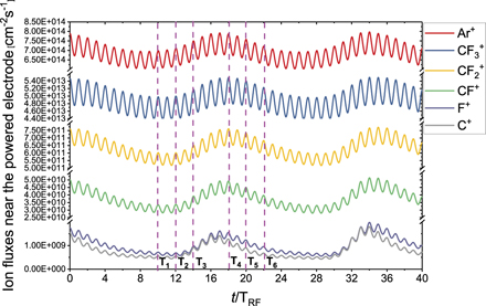
The presence of the plasma instabilities would be of more concern for plasma processing, while only supposing that the positive ion fluxes to the electrodes are significant for etching efficiency. We show in figure 9 periodic fluctuations of the ion fluxes at the powered electrode during more than two instability cycles, in the case of the shortest electrode gap of 2.8 cm. Under the simulation condition, the ion fluxes in ascending order are those of Ar+, CF3 +, CF2 +, CF+, F+, C+ respectively. As an example, the Ar+ flux, which dominates over the other fluxes, shows more than 23.08% difference between its maximum and minimum of the RF averaged values. We put the two extreme discharge states into our trench model [56] to explore the effect of this instability on etching, and find that the etching rate may experience a fluctuation of about 16%, which is more likely to give rise to inconsistent processing and might not be beneficial to a repeatable etching. It is worth mentioning that this fast oscillation on a time scale of microsecond was also observed and called B mode in an experimental work about control of instabilities in inductively coupled electronegative plasmas [57]. This instabilities are also apt to occur in highly electronegative O2 and SF6 discharges with higher electron temperature and instability growth rate. However, this quick B mode instability was not considered to be important in plasma processing until now due to the slow ion response time compared to the instability period.
Figure 9. Time evolution of ion fluxes at the powered electrode. The discharge conditions are the same as figure 1.
Download figure:
Standard image High-resolution image
4. Conclusions
In this paper, a one-dimensional fluid/Monte-Carlo (MC) hybrid model is adopted to investigate the periodic instability of RF CCP discharges in CF4/Ar mixtures. Periodic fluctuations are observed in the densities of electrons and ions, being regular in time and amplitude, on the order of microseconds, while a modulation of the neutrals is hardly noticeable. Throughout the evolution processes, the negative ion and electron densities change in opposite trends, making the electronegativity oscillate up and down with time. As the electronegativity attains its maximum value, the drift field in the bulk becomes much enhanced as usually observed in highly electronegative discharges, leading to evident electron heating and effective electron production in the bulk. This strongly oscillating electron energy and higher mean electron temperature are maintained for several RF periods, during which the electron density increases significantly and overshoots to a much higher value. Similarly, as the electronegativity becomes low due to strong electron generation, a weaker bulk electric field and insufficient electron heating result in less ionization and less electron production. The electron temperature remains weakly oscillating and at a smaller mean value while the electron density keeps decreasing. That is, highly oscillating in electron temperature accompanied by an increase in electron density, or weakly oscillating in electron temperature and a decrease in electron density would give rise to a positive feedback to the formation of the instability.
Additionally, the spatio-temporal evolutions of the electron impact reaction rates as well as the mean electron energy are also discussed for further understanding of the electron dynamics. The rates are selected as examples of high energy electrons involved like Ar ionization and excitation rates, or low energy electrons involved like Ar* ionization rate and CF4 dissociative attachment rate for F− formation. Ever since the time at which the bulk electronegativity is high, the ionization and excitation rates gradually become more noticeable from the bulk center and get stronger near the sheath edge, suggesting electron acceleration from one sheath expansion to the opposite sheath collapse. This evident electron heating with the mean electron energy strongly oscillating in the bulk lasts until the bulk electron density increases to a much higher value. Then, with the fading of Ar ionization and excitation, Ar* ionization and CF4 dissociative attachment become prominent as the drift electric field and the mean electron energy are getting weaker. The electron production from the Ar* ionization may act as a supplement to that from the weakening Ar ionization, but is limited and can only keep the electron density at a higher value for several RF periods. In this work, the rate of CF4 dissociative attachment, as the main electron attachment process, is at least two orders of magnitude smaller than the rates of Ar ionization and excitation. Thus, compared with discharges in purely electronegative gas, it cannot be attributive to the electron attachment/detachment as the main reason for the generation of the instabilities. However, with the existence of electronegative CF4, the regularly changeable electron heating by the bulk electric field makes the densities of the charged particles and electronegativity oscillate self-consistently. Thus, the drift electric field in the bulk which is affected by the electronegativity plays a crucial role in the unstable electron dynamics in this study.
By analyzing all the main terms in the electron continuity equation, we find not only the reaction rate like the Ar ionization rate but also the divergence of the electron flux  are the two significant terms that determine the time variation of the electron density in the discharge center, in this hybrid simulation. During the time of growing electronegativity, it results from more electron outflow and negative ion inflow from/to the discharge center as well as the insufficient ionization. And in the process of the decreasing electronegativity, the electron density increase is mostly due to the enhanced electron generation by Ar ionization while the electron outflow and negative ion inflow become quite low. And with the balance of these two terms, the electron density exhibits its extreme values. That is the important issue different from the analysis based on the global model.
Furthermore, from the overview comparisons and discussion, as the gap distance increases, the fluctuation amplitudes of all the main discharge variables are getting smaller gradually, and the instability period becomes longer till unnoticeable. This conclusion is based on the fixed range of the deposited power density for a reasonable analysis. For smaller electrode gap driven by almost the same power, the drift electric field enhances evidently with the lack of enough conductive electrons or becomes quite weak as the electron density overshoots to a much higher value, playing an important role in this unstable discharge. We also notice more than 23.08% fluctuation of the Ar+ ion flux to the powered electrode and about 16% difference in the etching rate in the unstable discharge with the distance of electrodes at 2.8 cm, suggesting that this instability is detrimental to stable etching and should be taken into account.
At last, we observe instabilities in a capacitive discharge in CF4/Ar gas mixture on the basis of a one-dimensional hybrid simulation, but experimental validation is also expected though differences caused by diagnostic methods and RF matching system may be unresolved. More details such as the influence of changing external parameters on the instability phenomenon and the etching process will be carried out in our future work.
Acknowledgments
This work was supported by the National Natural Science Foundation of China (Grant Nos. 12020101005, 11975067), and the German Research Foundation in the frame of the project 'Electron heating in capacitive RF plasmas based on moments of the Boltzmann equation: from fundamental understanding to process control' (No. 428942393).
Data availability statement
All data that support the findings of this study are included within the article (and any supplementary files).