
Abstract
Simulation of the impact of charge-exchange (CX) reactions on beam ions in the Mega Amp Spherical Tokamak (MAST) Upgrade was compared to measurements carried out with a fission chamber (neutron fluxes) and a fast ion deuterium-alpha (FIDA) diagnostic. A simple model was developed to reconstruct the outer-midplane neutral density based on measurements of deuterium-alpha emission from edge neutrals, and on Thomson scattering measurements of electron density and temperature. The main computational tools used were the ASCOT orbit-following code and the FIDASIM code for producing synthetic FIDA signals. The neutral density reconstruction agrees qualitatively with SOLPS-ITER modelling and yields a synthetic passive FIDA signal that is consistent with measurement. When CX losses of beam ions are accounted for, predicted neutron emission rates are quantitatively more consistent with measurement. It was necessary to account for CX losses of beam ions in simulations to reproduce the measured passive FIDA signal quantitatively and qualitatively. The results suggest that the neutral density reconstruction is a good approximation, that CX with edge neutrals causes significant beam-ion losses in MAST Upgrade, typically 20% of beam power, and that the ASCOT fast-ion CX model can be used to accurately predict the redistribution and loss of beam ions due to CX.
Export citation and abstract BibTeX RIS

Original content from this work may be used under the terms of the Creative Commons Attribution 4.0 license. Any further distribution of this work must maintain attribution to the author(s) and the title of the work, journal citation and DOI.
1. Introduction
Fast ions in magnetically confined fusion plasmas can be redistributed and lost via charge exchange (CX) with background neutrals. CX losses decrease the effective heating power and current drive from fast ions, and when the fast atoms resulting from CX strike the device wall they can cause damage to sensitive plasma-facing components, impurity sputtering and wall erosion. CX with background neutrals caused significant losses of fast ions produced by neutral beam injection in the Mega Amp Spherical Tokamak (MAST) [1]. Based on observations in the first physics campaign (MU01) of MAST Upgrade (MAST-U) [2], significant CX losses of beam ions are suspected in the upgraded device as well. MAST-U, a schematic of which is shown in figure 1, is equipped with two neutral beams, one injected in the geometric midplane of the vacuum vessel ('on-axis'), the other around 65 cm above the midplane ('off-axis'). The generation of fusion neutrons by the off-axis beam was lower than that of the on-axis beam, with a difference somewhat larger than that expected from considerations of geometry, plasma density and temperature, and magnetohydrodynamic (MHD) activity [3]. Fast-ion driven mode activity was much lower when only the off-axis beam was on compared to when only the on-axis beam was on. These observations suggest that, in nearly MHD-quiescent plasmas, ions from the off-axis beam, which are more susceptible to being ionized on loss orbits and to CX, have worse confinement than ions from the on-axis beam, with a difference larger than expected from direct orbit losses alone. This motivated detailed analysis of the impact of CX on beam ions in MU01 by means of modelling. In this article, we investigate the extent to which the ASCOT orbit-following code [4, 5] can be used in conjunction with other modelling tools to model the impact of CX with edge neutrals and other background neutrals on beam ions in MAST-U. We also discuss what this investigation reveals about the impact of CX on the beam-ion distribution.

Figure 1. Annotated cross-sectional schematic of MAST Upgrade. Reprinted from [6], Copyright (2015), with permission from Elsevier.
Download figure:
Standard image High-resolution imageThe fast-ion CX model of ASCOT models the redistribution of fast ions due to neutralizing CX reactions with background neutrals. Reionization of the resulting fast CX neutrals in the plasma is also simulated. The model has previously been analytically verified and benchmarked against the fast-ion module NUBEAM [7] of the transport code TRANSP [8, 9], and its capabilities have been demonstrated in a predictive MAST-U scenario [10]. In this article, predictions by the ASCOT CX model are compared to experimental results from the MU01 campaign with the aim of validating the model. ASCOT is used in conjunction with the ASCOT Fusion Source Integrator (AFSI) [11] to predict neutron emission from the plasma, and predictions are compared to measurements carried out with a fission chamber on MAST-U [12]. In addition, ASCOT is used in conjunction with the synthetic diagnostics code FIDASIM [13] to simulate passive fast ion deuterium-alpha (FIDA) spectra, and the simulated spectra are compared to measurements carried out with the MAST-U FIDA system [14–16]. Comparison to TRANSP modelling is made as well.
Previous CX modelling has been performed using the 4th version of ASCOT (ASCOT4) [10]. The same CX model has been adapted and implemented in the 5th version of ASCOT (ASCOT5). AFSI has not yet been implemented for ASCOT5, and ASCOT4 has not been interfaced with FIDASIM. Therefore, both code versions were needed to perform the analysis for this article but not all analysis could be performed with both versions. The ASCOT-AFSI work to predict neutron emission was performed using ASCOT4, and the ASCOT-FIDASIM work to predict FIDA signals was performed using ASCOT5. The CX models of ASCOT4 and ASCOT5 were benchmarked, showing good agreement. A detailed report on the benchmark is given in appendix
To address the main physics question of how CX with neutrals impacts fast ions in MAST-U, knowledge of the neutral background is required. The outer-midplane neutral density in MAST-U was reconstructed from radial deuterium-alpha (D-alpha) measurements carried out using the HOMER camera [17] and from plasma electron density and temperature measurements performed using a Thomson scattering system [18]. The model developed for this neutral density reconstruction was dubbed BATS1D. The reconstruction was complicated by major uncertainties in the HOMER calibration. The BATS1D neutral density was compared to modelling carried out using the SOLPS-ITER code [19].
In section 2, a method is presented for reconstructing the outer-midplane neutral density and comparison is made to SOLPS-ITER modelling for MAST-U. In section 3, results are presented on the comparison of predicted and measured neutron emission. In section 4, results are presented on the comparison of simulated and measured passive FIDA signals. In section 5, results are summarized and conclusions are drawn and discussed.
2. Reconstructing neutral density in MAST-U
2.1. D-alpha and inverted KN1D
The kinetic transport code KN1D [20, 21] can be used to calculate 1D atomic and molecular density profiles in an ionizing plasma. However, the code requires as input the neutral pressure at the device wall. Since no fast ion gauges (FIGs) were operational during MU01 in autumn 2021, measurements of the neutral gas pressure were not available for this analysis. Another method for calculating neutral density was devised using deuterium-Balmer-alpha (D-alpha) measurements and an inverted KN1D algorithm.
Once KN1D has predicted the neutral densities, it estimates the Balmer-alpha emission from atoms excited by electron impact. The rate of photon emission in units of m−3 s−1 is calculated as [21]
where  is the spontaneous emission coefficient for protium-Balmer-alpha, which differs from that of D-alpha by only 0.03%, r03 and r13 are the recombination and ionization coefficients, respectively, from energy level 3, n0 is the ground-state atomic density, and
  and
and  are the Saha equilibrium population densities (m−3) for atomic hydrogen at the energy levels 1 (ground-state) and 3, respectively. The photon emissivity, in accordance with the Bohr model, is converted into emissivity in units of Wm−3 as
where E1 is the ground-state ionization energy of hydrogen in eV and e is the elementary charge in C. D-alpha emission on the midplane was measured in MU01 using the linear CCD camera HOMER [17], which features horizontal sightlines with tangency points ranging from the scrape-off-layer (SOL) through the plasma and through the centre column to the other side of it, allowing for the calculation of a radially resolved D-alpha emissivity profile. This provides the emissivity ε in equation (2). Equations (1) and (2) were rearranged such that ground-state atomic density could be calculated from D-alpha emissivity. First the emissivity is converted into a photon emission rate  using equation (2). Then, rearranging equation (1), the ground-state atomic density is calculated as
The atomic density on the outer midplane in MAST-U can be estimated using equations (2) and (3) by inserting Thomson scattering data for the electron density and temperature on the midplane, and D-alpha measurements on the midplane obtained using the HOMER camera. In equation (3), the electron density and temperature are used to evaluate the parameters r03, r13,  and
and  . This model, which uses Balmer-Alpha and Thomson Scattering data in inverted equations from the KN1D code, was dubbed BATS1D. A similar method has been used to estimate the outer-midplane neutral density in NSTX-U [22].
Atoms excited by molecular dissociative processes contribute to the D-alpha emission, especially in the SOL [22]. In the above described model, specifically the inverted KN1D equations, the atomic density is estimated based on the assumption that the full emissivity measured by HOMER results from atoms excited by electron impact. Therefore, the calculated atomic density is an upper estimate for the true atomic density. In the NSTX-U study, there was evidence to suggest that a similar upper estimate tracked closely the true atomic density in the plasma, where molecular density is expected to be low, and that the upper estimate tracked closely the sum of atomic and molecular density in the SOL, where molecular density is expected to be significant [22]. It is reasonable then to assume that a BATS1D-calculated upper estimate for the atomic density is, in fact, an estimate for the total neutral density. Furthermore, at temperatures typical in the plasma edge and SOL, between 1 eV and 100 eV, in an energy range relevant for fast-ion CX in MU01, between 10 keV and 70 keV, the reaction probability is similar for CX with deuterium atoms and molecules. Under these conditions, the reaction rate coefficients for CX between a deuteron and a Maxwellian deuterium atom, and between a deuteron and a Maxwellian deuterium molecule, when the molecule starts in the vibrational ground state and ends up in any vibrational state, agree to within 50%, such that the probability for CX with a molecule is 0%–50% higher [10, 23]. Therefore, when simulating beam-ion CX in MAST-U, it would be a good approximation to consider a neutral background consisting of atoms and molecules as a neutral background consisting purely of atoms, assuming an atomic density equalling the sum of the true atomic and molecular densities. The BATS1D model, which includes D-alpha light from all sources, produces an approximation of such a total neutral density that includes both atoms and molecules. It should be noted that the plasma edge and SOL contain molecular ions as well. However, according to KN1D modelling performed for experiments from the second physics campaign (MU02) of MAST-U for this article and according to literature, their density is typically at most one tenth of the neutral density, so they can be neglected [22].
2.2. Constructing neutral density profiles
BATS1D and the TRANSP internal neutral model FRANTIC were used to reconstruct the outer-midplane neutral deuterium density in two MU01 shots: in shot 44623 at times 0.31, 0.32, 0.33, 0.39, 0.40 and 0.41 s, and in shot 45091 at time 0.35 s. The neutral density estimates were used in ASCOT4 modelling of shot 44623 to compare predicted and measured neutron rates, which is reported in section 3, as well as in ASCOT5 and FIDASIM modelling of shot 45091 to compare predicted and measured passive FIDA signals, which is reported in section 4. In addition, BATS1D modelling was performed for shot 45469 at time 0.40 to compare the result to SOLPS-ITER modelling. The analysed MU01 cases are listed in table 1, with brief comments on the type of plasma and what the cases were used for. The final neutral density profiles for shot 44623 at the example time 0.40 s and for shot 45091 at time 0.35 s are shown in figure 2, and the reconstruction process is explained below.

Figure 2. Outer-midplane neutral deuterium density reconstructions for shot 44623 at time 0.40 s (a) and shot 45091 at 0.35 s (b) as functions of the normalized poloidal flux  , where
  is the poloidal flux, and
  and
and  are its values at the magnetic axis and inside the separatrix, respectively. In (a), BATS1D part based on proxy shot 44578 at 0.32 s. Extrapolation of maximum BATS1D value in yellow. Best-estimate profile shown using solid lines, limiting-estimate profiles using shaded colour bands. In (a), TRANSP-part version that was not scaled to BATS1D part is shown using dashed orange line. In (b), TRANSP-part version with both wall atoms and recombination atoms shown using solid orange line and orange colour band, while best-estimate TRANSP-part version with only wall atoms is shown using dashed orange line.
Download figure:
Standard image High-resolution imageTable 1. A list of the analysed MU01 cases in terms of shot number and time point. The plasma type is indicated as a confinement mode or heating scheme. The fourth column briefly describes what the case was used for.
| Type | Shot | Time (s) | Usage |
|---|---|---|---|
| H-mode | 44578 | 0.32 | Proxy for 44623 neutrals |
| 44623 | 0.31–0.41 | Analyse neutrons | |
| L-mode | 45091 | 0.35 | Analyse passive FIDA |
| Ohmic | 45469 | 0.40 | Compare to SOLPS-ITER |
Due to uncertainties in both the spatial and brightness calibrations of the HOMER camera in MAST-U, the BATS1D model introduced in section 2.1 could not be directly used. The uncertainties were circumvented with ad hoc solutions that are detailed in appendix
To test the BATS1D model, including the extra corrections described in appendix
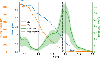
Figure 3. Outer-midplane HOMER D-alpha and Thomson scattering electron density ne and temperature Te data used for estimating the neutral density in shot 45469 at 0.40 s, plotted as functions of major radius. For the D-alpha profile, the result when scaling with the best-estimate scaling factor for this case, 4.8, is shown with the solid green line. The results using the minimum and maximum scaling factors, 2.2 and 5.6, respectively, are indicated using a shaded green band.
Download figure:
Standard image High-resolution imageDue to an interruption in the camera operation, there are no HOMER data for shot 44623. The similar case of shot 44578 at time 0.32 s was used as a proxy. Similarity was judged in the same way as in appendix
Based on the comparison to SOLPS-ITER in appendix  = 0.95–0.99, where the inner limit of the validity of the BATS1D model is expected to be based on the comparison to SOLPS-ITER. While the BATS1D estimate for the time point 0.32 s was used for the BATS1D parts of the neutral density profiles for shot 44623 at all six time points, the TRANSP parts of the profiles were taken from the correct time points in the TRANSP simulation for shot 44623. At all six times of the TRANSP simulation for shot 44623, and with all three scaling factors for the BATS1D reconstruction for shot 44578 at 0.32 s, the profile slopes match best at
  = 0.97. For shot 45091 at time 0.35 s, for all six combinations of the two versions of the TRANSP profile and the three scaling factors for the BATS1D reconstruction, the profile slopes match best at
  = 0.98. After choosing the junction, the TRANSP profiles were scaled with a constant factor such that they equal the corresponding BATS1D profile at the junction.
The TRANSP parts of the neutral density profiles are shown in orange in figure 2. For shot 44623, the full atomic density from TRANSP was used, which means that atoms were included from all three of the simulated sources: atoms recycled from the wall, beam-halo atoms and atoms born in recombination reactions in the plasma. Since the analysis of shot 45091 is based on measurements by the passive FIDA diagnostic, whose sightlines are on the opposite side of the plasma from the neutral beam sightlines by design, the beam-halo atoms were omitted from the TRANSP atomic density profile for this shot. Furthermore, for a more comprehensive investigation, two of the remaining alternative versions of the TRANSP atomic density were used: one with both wall atoms and recombination atoms, and one with only wall atoms. In figure 2(b), the best-estimate and limiting-estimate profiles with both wall atoms and recombination atoms are shown using the solid orange line and shaded orange colour band, respectively, while the best-estimate profile with only wall atoms is shown using a dashed orange line.
The described use of the TRANSP neutral density deeper inside the plasma has not been validated. However, since most CX losses of beam ions result from neutralizations in the SOL and the very edge of the plasma, the neutral density profile deeper inside the plasma is not expected to have a significant impact on the beam-ion confinement, unless the neutral density is greatly overestimated. To test this, versions of the best-estimate neutral density profiles for shot 44623 were constructed where the TRANSP part was not scaled to the BATS1D part. In the example of shot 44623 at 0.40 s in figure 2(a), this is shown using a dashed orange line. The impact of using these profiles instead of those where the TRANSP part is scaled is reported in section 3. In the analysis of shot 45091, neutrals impact not only the redistribution of beam ions but also the generation of FIDA light. That makes the analysis more sensitive to the reconstruction of the neutral density deeper inside the plasma, but also provides an opportunity to validate the reconstruction. This is further discussed in section 4.
In the SOL, the validity of the BATS1D model ends where the electron density drops to near-zero values. For the neutral density reconstruction, the profile calculated by BATS1D was used up to its maximum value. Further out, this maximum value was used as a constant extrapolate. This extrapolated part of the profile is shown in yellow in figure 2. Both for shot 44578 at 0.32 s and 45091 at 0.35 s, the maximum is reached within 5 cm of the separatrix at the outer midplane, where 5 cm outside the separatrix corresponds to about  = 1.1. According to the KN1D modelling done for MU02 cases in appendix
  = 1.1–1.2. Based on these observations, the extrapolated parts of the reconstructed neutral density profiles are underestimations. This SOL region is relevant, since beam ions on the outer midplane in MAST-U have gyroradii of up to 10 cm.
The neutral density distributions constructed as described above and used in the modelling reported in sections 3 and 4 were assumed to be poloidally uniform. Each reconstructed outer-midplane density was used for the whole plasma and SOL as a 1D density function along  . The assumption of poloidal uniformity is probably not correct, due to strong recycling from the divertors and neutral gas from the fuelling valves. However, because of a pronounced Shafranov shift, strong orbit drifts and strongly major-radius-dependent gyroradii, fast ions in MAST-U have orbits that are weighted towards the low-field side of the plasma [10]. This is illustrated in figure 4, which shows the beam-ion distribution in the (R, z) plane in shot 44623 at 0.39 s when both the on- and off-axis beams are on, as predicted by ASCOT4 when CX reactions are not accounted for. The beam-ion density is essentially zero in the very top and very bottom of the plasma as well as near the edge on the high-field side. This is expected to limit the interactions of the beam ions with the higher neutral densities towards the divertors and high-field-side fuelling valves. The beam-ion population overlaps with the relatively high neutral density levels of the plasma edge and SOL on the low-field side, in particular on the outer midplane, which is where the neutral density reconstruction was calculated. Finally, the passive FIDA diagnostic, used for the analysis of shot 45091, views the outer midplane. These observations imply that error introduced by assuming a poloidally uniform neutral density is significantly mitigated. Therefore, the approximation is deemed good for the analysis performed in this article.

Figure 4. Beam-ion density predicted by ASCOT4 in shot 44623 at 0.39 s when CX reactions are not accounted for. Equilibrium contours for  = 0.2, 0.4, 0.6, 0.8 and 1.2 in grey and for
  = 1.0 in red, and the 2D wall representation in black are indicated.
Download figure:
Standard image High-resolution image3. Comparing predicted and measured neutron rates
During the MU01 campaign, a fission chamber was operated outside the tokamak in toroidal sector 11 to measure the total neutron emission rate from the plasma [12]. Neutron rate predictions made by combined modelling using ASCOT4 and AFSI were compared to fission chamber measurements to validate the ASCOT4 CX model and to investigate the impact of CX on beam-ion confinement. As a benchmark exercise, ASCOT4-AFSI and TRANSP predictions of neutron rates were also compared. The 4th version of ASCOT was chosen for this study since the corresponding AFSI version was ready for use and has been validated and widely used in previous work [11, 24–26].
For this analysis, the MU01 shot 44623 (same as in appendix  = 0.7 and 0.8.
There is uncertainty in the absolute calibration of the fission chamber. ASCOT4-AFSI and TRANSP both predict neutron rates that are higher by a factor of 2–4 than those measured by the fission chamber for shots from MU01. Experts at MAST-U conducted a comprehensive study where the total neutron emission, cumulated over the time that the neutral beams were on, was measured by the fission chamber and predicted by TRANSP in nine MU01 shots. Comparing the measurements and predictions, the experts derived an additional scaling factor of 3.0 for the fission chamber, which was applied to measurements from MU02. Since TRANSP commonly underestimates fast-ion losses, the experts expect this scaling factor to cause an overestimation of the measured neutron emission. This scaling factor was applied to the fission chamber measurements for MU01 shot 44623 for the analysis reported in this article.
The ASCOT4 simulations for the present section were prepared based on the same TRANSP simulation and in the same way as in appendix
Unlike in the comparison to fission chamber measurements, when ASCOT4-AFSI was compared to TRANSP, the TRANSP neutral density was used also in the ASCOT4 CX model. The ASCOT4-AFSI neutron emission predictions agree with TRANSP to within 7%, as shown in figure 5.

Figure 5. Total neutron rate from the plasma in shot 44623 as predicted by ASCOT4-AFSI and TRANSP using the TRANSP neutral density and including CX.
Download figure:
Standard image High-resolution imageFor the comparison of neutron predictions by ASCOT4-AFSI and measurements by the fission chamber, the neutral density profiles reconstructed using BATS1D (and TRANSP for deeper inside plasma, figure 2(a)) were used when simulating CX in ASCOT4. Before comparing predicted and measured neutron rates, the sensitivity of the ASCOT4-AFSI prediction to the neutral density deeper inside the plasma was tested using alternative neutral density profiles, whose construction was explained in section 2.2. For each of the six analysed time points in shot 44623, ASCOT4 simulations with CX included were compared for two variants of those neutral density profiles where the HOMER-measured D-alpha emissivity was scaled with the best-estimate factor of 5.0: one variant where the density profile deeper inside the plasma (part calculated by TRANSP) is scaled to the density profile at the edge (part calculated by BATS1D), and one variant where it is not scaled. Examples of these variants are shown in figure 2(a) using a solid and a dashed orange line, respectively. Only minor differences were observed in the simulation results. Taking as an example the simulation of the time point 0.39 s, the predicted fast-ion density profiles as functions of  agree to within 3% outside
  = 0.3. In the core, the fast-ion density is at most 8% lower for the case where the TRANSP part of the neutral density profile was scaled. When the TRANSP part was scaled, the loss of beam power was 3% higher. Throughout the six time points simulated, the predicted neutron rates agree to within 1% when using the two variants of the neutral density profile. In the following analysis, those neutral density profiles were used where the TRANSP part was scaled to the BATS1D part.
In the ASCOT4 simulations, of the power in beam particles ionized in the plasma (excludes shine-through), practically all loss occurs as direct orbit losses and, when the CX model is on, due to CX with background neutrals. When only the off-axis beam is on, ASCOT4 predicts that 8%–9% of the power is lost when CX is off and 45%–46% when CX is simulated using the best-estimate neutral profiles, 34%–47% when the limiting-estimate cases are included. When both beams are on, ASCOT4 predicts that 10%–11% of the power is lost when CX is off and 32% when CX is simulated using the best-estimate neutral profiles, 25%–33% when the limiting-estimate cases are included. As expected, the relative CX losses are higher when only the off-axis beam is on, since ions from the off-axis beam are more susceptible to CX. All else being equal, it would also be expected that the relative amount of direct orbit losses is higher when only the off-axis beam is on. However, in the latter analysed time period when both beams are on, the low-field side separatrix is closer to the device wall, by 3 cm on the outer midplane, which explains the higher direct orbit losses.
Figure 6 compares the neutron predictions by ASCOT4-AFSI, with and without CX included in the ASCOT4 simulations, to the neutron measurements by the fission chamber. The predictions when CX was simulated using the best-estimate neutral profiles are shown using blue dots and the limiting-estimate cases are indicated with blue error bars. When only the off-axis beam is on, ASCOT4-AFSI overestimates the measured neutron rate by 38%–47% when CX is off and by 6.0%–11% when CX is simulated using the best-estimate neutral profiles, by 3.5%–25% when the limiting-estimate cases are included. When both beams are on, ASCOT4-AFSI overestimates the measured neutron rate by 29%–42% when CX is off and by 18%–29% when CX is simulated using the best-estimate neutral profiles, by 18%–34% when the limiting-estimate cases are included. When calculating the above quoted differences at the simulated time points, the fission chamber data were time-averaged 5 ms in each direction.
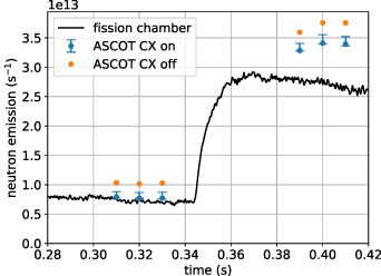
Figure 6. Total neutron rate from the plasma in shot 44623 as measured by the fission chamber, with an additional scaling factor of 3.0, and as predicted by ASCOT4-AFSI, with and without the inclusion of CX. CX was simulated using the neutral density reconstructions based on BATS1D calculations. Predictions when CX was simulated using the best-estimate neutral profiles are shown using blue dots and the limiting-estimate cases are indicated with blue error bars.
Download figure:
Standard image High-resolution imageThe predicted neutron emission rates are consistently higher than the measured, but only modestly when only the off-axis beam is on and CX is accounted for, as shown in figure 6. The overestimation could mean that the fission chamber calibration is still incorrect, perhaps an additional scaling factor higher than the factor 3.0 used here is needed to raise the signal to the true level. It could also mean that the ASCOT4 modelling is underestimating beam-ion losses. Perhaps the estimated neutral density is too low, or perhaps significant beam-ion losses are caused by a mechanism not captured by the modelling. As was discussed in section 2 and appendix
When only the off-axis beam is on and the plasma is MHD-quiescent, accounting for CX substantially improves the quantitative agreement between predicted and measured neutron emission. This result indicates that CX has a significant impact on beam-ion confinement in MAST-U, and that the ASCOT4 CX model is able to reproduce this effect. However, the result will have to be verified once the fission chamber has been calibrated. When both beams are on, accounting for CX does not significantly improve the agreement between prediction and measurement, apparently due to additional fast-ion losses caused by a mode excited by the on-axis beam. The analysis of this time period cannot be used to validate the CX model. However, it demonstrates a situation where reliable modelling of CX losses could help provide more information about a fast-ion driven mode. If direct orbit and CX losses are predicted correctly, the remaining difference between the simulated and measured neutron rates is a more accurate measure of the effects of the mode on the fast ions.
4. Comparing predicted and measured passive FIDA
MAST-U is equipped with an 11-channel FIDA system with both an active view, in the same plane as and intersecting with the on-axis beam, and a passive view, which does not overlap with any beam [14–16]. When the bremsstrahlung background is accounted for and a relevant wavelength interval is investigated, FIDA light from CX between fast ions and edge neutrals can be observed if the overlap between the fast-ion population and edge neutrals is large enough [27–29]. This overlap is larger in MAST-U than, for example, in ASDEX Upgrade due to the larger fast-ion gyroradii in MAST-U. Hence, significant passive beam-ion FIDA light is expected in MAST-U. Since the redistribution and loss of beam ions due to CX with background neutrals predominantly affects the beam-ion distribution function near the edge, analysis of passive FIDA can be expected to capture these effects. There exists an established methodology for using TRANSP and FIDASIM modelling to compare simulated fast-ion distributions to experiments based on measurements of FIDA intensity in MAST and MAST-U, and the FIDA system has been absolutely calibrated [14–16].
In this study, passive FIDA intensity was predicted using combined modelling with ASCOT5 and FIDASIM. The predictions were compared to measurement to validate the ASCOT5 CX model and to investigate the impact of CX on the beam-ion distribution. The 5th version of ASCOT was chosen because of a pre-existing interface program in the ASCOT5 code library [5] that was used to insert the ASCOT5-predicted beam-ion distribution functions and scenario inputs into FIDASIM. To verify the ASCOT5-FIDASIM modelling scheme, its predictions were compared to those of the established TRANSP-FIDASIM scheme, in which case the TRANSP neutral density was used also in ASCOT5.
For this analysis, the MU01 shot 45091 was chosen: a double-null, L-mode plasma with 600 kA of plasma current and a conventional divertor configuration. The time point 0.35 s, when both beams are on, was chosen because of its relative MHD-quiescence. The case was first reconstructed similarly as in appendix
As an example, figure 7 shows the ASCOT5-FIDASIM-simulated and measured passive FIDA spectra for channel 9 out of 11, with the bremsstrahlung background subtracted from the measured spectrum to reveal the underlying beam-ion FIDA signal. The major radius coordinate of the tangency point (tangency radius) of the sightline for channel 9 is 1.29 m, which corresponds to  = 0.70 in shot 45091 at time 0.35 s. The bremsstrahlung emissivity, which is not expected to vary significantly over the entire range of the plotted spectrum (down to 656 nm), was estimated by taking the signal average between 662.0 and 662.4 nm, which is beyond the possible wavelengths from beam-ion D-alpha in this case. The maximum beam-ion energy, i.e. the full energy of the off-axis beam, was 72.5 keV, which yields a maximum Doppler-shifted D-alpha wavelength of 661.9 nm. Indeed, the simulated and the bremsstrahlung-corrected measured spectra drop off below that wavelength. The peaking in the measurement at wavelengths below 659.0 nm is caused by the two passive carbon lines at 657.8 and 658.3 nm. The measurement error is based on the known photon statistics properties, and is part of the established methodology of FIDA measurement at MAST-U [14–16]. Error from the bremsstrahlung subtraction, accounting for the averaging using the formula for the standard error of the mean, was added to the final error margins.

Figure 7. ASCOT5-FIDASIM-simulated and measured passive FIDA spectra (logarithmic scale) for channel 9 (out of 11 channels), with tangency radius 1.29 m ( = 0.70), in shot 45091 at 0.35 s. Bremsstrahlung has been estimated as the signal average between 662.0 and 662.4 nm and subtracted from the measured spectrum. Predictions using the best-estimate neutral profile whose TRANSP part includes recombination atoms are shown using solid lines. The corresponding limiting-estimate cases are indicated with shaded colour bands.
Download figure:
Standard image High-resolution imageThe simulated results shown in figure 7 are based on those best-estimate and limiting-estimate neutral profiles whose TRANSP parts include recombination atoms. At channel 9, between the carbon lines and the upper limit of the Doppler shift, the prediction when CX is simulated using the best-estimate neutral profile in ASCOT5 mostly agrees with the measurement. If the predictions based on the limiting-estimate neutral profiles are viewed as error margins, there is complete agreement between prediction and measurement. When CX is not accounted for in ASCOT5, the best-estimate neutral profile is used in FIDASIM, and wavelengths between 659.0 and 661.0 nm are considered, the prediction is about three times as high as the measurement. To plot the passive FIDA signals as radial functions in the following analysis, the spectrum from each channel was simplified into a single intensity value by averaging over the relatively flat range between wavelengths 659.0 and 661.0 nm. The choice of wavelength range avoids the two carbon lines and the high noise-to-signal ratio in the drop of the spectrum past 661.0 nm. The measurement error from each spectrum was propagated through the calculation, accounting for the averaging using the formula for the standard error of the mean.
Figure 8 shows the passive FIDA signals predicted by ASCOT5-FIDASIM and TRANSP-FIDASIM as functions of the tangency radii of the FIDA channels. In the FIDASIM simulations for this code comparison, beam-halo and recombination atoms from the TRANSP neutral background were omitted, and regions outside the separatrix were omitted completely using artificial masking, i.e. the signal contribution from outside the separatrix was set to zero, as has been common practice in TRANSP-FIDASIM modelling of active FIDA in MAST and MAST-U [14, 15]. While active FIDA is predominantly produced by CX from the excited state n = 3 (n is the principal quantum number) in a fast beam neutral or a beam-halo neutral to the state n = 3 in a neutralized fast ion, passive FIDA is predominantly produced by CX directly from the ground state (n = 1) in a background neutral to the state n = 3 in a neutralized fast ion. Therefore, a substantial contribution to the passive FIDA signal can come from the SOL even when the electron density and temperature are negligible. Passive FIDA from the SOL is accounted for in the comparison to measurement.

Figure 8. Passive FIDA signals in shot 45091 at 0.35 s predicted by ASCOT5-FIDASIM and TRANSP-FIDASIM as functions of the tangency radii of the FIDA channels (corresponding  coordinates range from
  = 0.47 on the high-field side to
  = 0.95 on the low-field side). For each model and each channel, the passive FIDA spectrum has been averaged between wavelengths 659.0 and 661.0 nm.
Download figure:
Standard image High-resolution imageIn the code comparison, the ASCOT5-FIDASIM prediction for the passive FIDA signal agrees with the TRANSP-FIDASIM prediction to within 30%, except at the outermost point where the ASCOT5-FIDASIM prediction is 50% lower, as shown in figure 8. The channel numbering, 1–11, runs from lowest to highest major radius. In shot 45091 at 0.35 s, channels 1–4 have tangency points on the high-field side, while channels 5–11 have tangency points on the low-field side, as shown in figure 10. Based on the data shown in figures 8 and 9, channel 1 appears spurious. On the low-field side, the ASCOT5-FIDASIM and TRANSP-FIDASIM predictions shown in figure 8 start to diverge at channel 6. The ASCOT5-estimated fast-ion density as a function of  agrees with that of TRANSP to within 10% across
  values corresponding to the tangency points of channels 6–10. However, at the tangency point of channel 11, the ASCOT5 value is only 30% of the TRANSP value. Both fast-ion density functions have very low values this close to the edge when CX is accounted for. The values at the tangency point of channel 11, which corresponds to
  = 0.95, are 0.3% and 0.9% of the values at
  = 0.50 for ASCOT5 and TRANSP, respectively. This means that the simulation statistics are poor in this part of the distribution function. Since the passive FIDA signal is dominated by FIDA light from the edge for any channel [27], the substantial relative difference in the fast-ion density functions on the very edge likely explains most of the differences in the synthetic passive FIDA signals not only at channel 11 but also at channels 6–10. While the bright edge affects all channels, a lower tangency radius still implies a more radial sightline, which implies more signal contribution from deeper inside the plasma [14]. This may explain why the passive FIDA predictions differ noticeably but not strongly at channels 6–10. The demonstrated level of agreement with the established TRANSP-FIDASIM model and the identification of an explanation for the modest differences that were observed suggest that the ASCOT5-FIDASIM modelling works and can give physically accurate predictions of the passive FIDA signal in MAST-U.
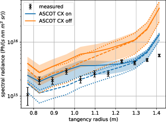
Figure 9. ASCOT5-FIDASIM-simulated and bremsstrahlung-corrected measured passive FIDA signals (logarithmic scale) in shot 45091 at 0.35 s as functions of the tangency radii of the FIDA channels. For each channel, the simulated and measured passive FIDA spectra have been averaged between wavelengths 659.0 and 661.0 nm. Predictions using the best-estimate neutral profile whose TRANSP part includes recombination atoms are shown using solid lines. The corresponding limiting-estimate cases are indicated with shaded colour bands. Predictions using the best-estimate neutral profile excluding recombination atoms are shown using dashed lines. The corresponding limiting-estimate cases are indicated with dotted lines.
Download figure:
Standard image High-resolution image
Figure 10. Ratio between the beam-ion density around the outer midplane in shot 45091 at 0.35 s predicted by ASCOT5 when CX is off and the one predicted when CX is simulated using the best-estimate neutral density profile whose TRANSP part includes recombination atoms. Equilibrium is illustrated using contours for  = 0.2, 0.4, 0.6, 0.8 and 1.2 in grey and for
  = 1.0 in red. Tangency points of FIDA channels are indicated by black crosses.
Download figure:
Standard image High-resolution imageFigure 9 shows the ASCOT5-FIDASIM-predicted, with and without CX, and bremsstrahlung-corrected measured passive FIDA signals as functions of tangency radius. In these FIDASIM simulations, artificial masking was applied only to regions outside  = 1.2, which should be out of reach of any beam ions and, therefore, irrelevant. The ASCOT5-FIDASIM modelling, both with and without CX included in ASCOT5, was performed using the six different neutral profiles constructed in section 2.2. Predictions with CX on are shown in blue and those with CX off in orange. The predictions using the best-estimate neutral profile whose TRANSP part includes recombination atoms are shown using solid lines. The corresponding limiting-estimate cases are indicated with shaded colour bands to reflect that they are interpreted as error margins. The predictions using the best-estimate neutral profile whose TRANSP part excludes recombination atoms are shown using dashed lines. The corresponding limiting-estimate cases are indicated with dotted lines. The cases with the minimum-estimate neutral densities consistently yield the lowest passive FIDA signals and the cases with the maximum-estimate neutral densities yield the highest passive FIDA signals.
Based on the data shown in figures 8 and 9, channel 1 appears spurious. At the outermost channel, channel 11, all predictions shown in figure 9 diverge from the measurement due to peaking in the predicted signals. It is unclear why the predictions overestimate peaking at the edge, but possible explanations were identified. As was discussed in section 2 and appendix
When CX reactions are included in the ASCOT5 simulation, the predicted passive FIDA signal is quantitatively more consistent with the measurement, in particular at higher tangency radii, as shown in figure 9. If we consider the best-estimate cases with and without recombination atoms as two alternative predictions whose error margins are determined by the corresponding limiting-estimate cases, then one or both of the predictions agree with the measurements at all channels 2–10 within error margins when CX is accounted for. This result suggests that the neutral density reconstructions are good approximations of the true neutral background. Specifically, it lends credibility to the decision in section 2.2 to scale the TRANSP part of the neutral density profile to the BATS1D part since, unlike in the neutron analysis in section 3, here the accuracy of the neutral density deeper inside the plasma is important because of its effect on the production of passive FIDA light. For shot 45091 at 0.35 s, the TRANSP-part neutral density was higher before scaling, even in the case of the maximum estimate from BATS1D. The result of the comparison of simulated and measured passive FIDA further indicates that, given an accurate neutral background density, the ASCOT5 CX model is able to capture the impact of CX on the beam-ion distribution.
Proceeding to more detailed analysis of the results shown in figure 9, predictions where ASCOT5 accounts for CX agree with measurement at channels 2–4 and 6–10 when recombination atoms are included. There is good agreement at channel 5 when recombination atoms are excluded. In addition, there is considerably better agreement at channels 6 and 7 when recombination atoms are excluded. These results suggest that there is a significant population of background neutrals from recombination, or some other source, deeper inside the plasma, but that the TRANSP neutral model is only partially successful in reproducing it, or that the TRANSP neutrals have been incorrectly incorporated in the neutral reconstruction in this article. Alternatively, considering the 3D shape of the plasma that the FIDA sightlines pass through, perhaps the FIDASIM modelling is overestimating a signal contribution from the edge on the far side of the plasma by underestimating the opacity of the plasma. This may explain why the predicted signals show a downward trend from channel 7 towards lower radii to channel 2, whereas the measured signal is quite constant across these channels. The tangency points of channels 2–4 and 5–7 lie quite symmetrically on either side of the magnetic axis, as shown in figure 10. Overestimating a signal contribution from the far side of the plasma may also explain why the predictions peak excessively at the edge.
When CX reactions are not included in the ASCOT5 simulation, the measured passive FIDA signal is significantly overestimated, in particular at higher tangency radii, as shown in figure 9. When the best-estimate neutral profile with recombination atoms is used in FIDASIM but CX is not accounted for in ASCOT5, the predicted passive FIDA signal at channels 2–10 is 1.4–3.8 times as high as the measured signal. At channels 5–10, i.e. the channels with tangency points on the low-field side, the ratio is 2.1–3.8. When CX is accounted for in ASCOT5, the ratio of prediction to measurement is 0.9–1.8, both at all channels 2–10 and at only channels 5–10. The better performance of ASCOT5 simulations where CX is accounted for is explained by the difference in the simulated beam-ion density near the edge. Figure 10 shows the ratio of the ASCOT5-estimated beam-ion density on the outer midplane when CX is off to the one when CX is on. Around the outer-midplane separatrix, the beam-ion density is estimated to be two to four times as high when CX reactions are neglected, which is consistent with the difference predicted in the passive FIDA signal. This result indicates that CX has a significant impact on beam-ion confinement in MAST-U, and that the ASCOT5 CX model is able to reproduce this effect. The figure shows the tangency points of the eleven FIDA channels. The set of tangency points runs from the high-field side, through the axis, and along the outer midplane to the low-field-side edge. One should keep in mind, however, that since passive FIDA light is edge-localized, even the signal in the inner channels comes predominantly from where their respective sightlines cross the edge [27]. Since this is the passive FIDA view in MAST-U, there is no contamination from active FIDA from interactions between fast ions and a beam line.
To complement the above, mainly quantitative analysis, the shapes of ASCOT5-FIDASIM-simulated passive FIDA spectra, with and without accounting for CX in the ASCOT5 simulation, were compared to the shapes of measured spectra. The spectra were normalized such that each spectrum was divided by its average value between wavelengths 659.0 and 661.0 nm. For the measured spectra, the relative error of the average value, calculated using the formula for the standard error of the mean, was added to the existing relative error at each point in the spectrum. The graphs for the normalized spectra predicted using the best-estimate and limiting-estimate neutral density profiles were merged into a single colour band whose borders at each wavelength are the minimum and maximum values from across the three individual spectra. At channels 2–7, the difference between the normalized spectra predicted with and without CX is so small compared to the error in the measured spectrum that no conclusions can be drawn. At channels 8 and 9, a statistically significant difference is emerging, and at channels 10 and 11 the difference is clear, as shown in figure 11. When CX is not accounted for, the drop of the spectrum past the wavelength 660.5 nm begins at too low wavelengths, meaning that there is proportionally to little highly Doppler-shifted FIDA light. When CX is accounted for, the drop of the spectrum mostly agrees with measurement. Figure 11 shows data from simulations using those neutral density profiles whose TRANSP parts include recombination atoms, but the results were not significantly different when excluding recombination atoms. This comparison of normalized passive FIDA spectra shows that predictions agree qualitatively better with measurement if CX is accounted for when simulating the beam-ion distribution function. The measured spectra appear to exhibit some oscillation at wavelengths below 661.0 nm, the reason for which is unclear. The oscillation is not reproduced in the predicted spectra, resulting in somewhat weaker agreement with measurement at these wavelengths, especially at channel 11.

Figure 11. Normalized ASCOT5-FIDASIM-simulated and bremsstrahlung-corrected measured passive FIDA spectra (logarithmic scale) for channels 8 (a), 9 (b), 10 (c) and 11 (d) (out of 11 channels) in shot 45091 at 0.35 s. Each spectrum was normalized by division with its average value between wavelengths 659.0 and 661.0 nm. Graphs for the normalized spectra predicted using the best-estimate and limiting-estimate neutral density profiles were merged into a single colour band whose borders at each wavelength are the minimum and maximum values from across the three individual spectra. Those neutral density profiles were used whose TRANSP parts include recombination atoms.
Download figure:
Standard image High-resolution imageThe better qualitative agreement with measurement when accounting for CX in simulations is explained by the impact of CX on the velocity-space distribution function near the edge on the outer midplane. Figure 12 compares the beam-ion distribution functions calculated by ASCOT5 with and without CX as functions of particle energy and pitch in the limited spatial domain where R = 1.33–1.60 m and z = −0.10–0.10 m, covering the outer midplane from between channels 9 and 10 to well outside the plasma, as seen in figure 10. CX was simulated using the best-estimate neutral density profile whose TRANSP part includes recombination atoms. Figure 12 shows that a large part of the beam-ion population is lost due to CX. More importantly for this analysis, it shows that the shape of the distribution function is altered by CX. When CX is accounted for, there are proportionally more beam ions with high energy and highly negative pitch, i.e. ones that have only recently been injected. The reason is that many of the beam particles ionized this close to the edge only have a short time to contribute to the distribution function before being lost due to CX. This is consistent with figure 11, where the spectra predicted when CX is accounted for feature proportionally more highly Doppler-shifted FIDA light. The observation that predicted passive FIDA spectra agree qualitatively better with measurement when CX is accounted for, and the identification of an explanation for this, provide further evidence that the ASCOT5 CX model is able to capture the impact of CX on the beam-ion distribution. These results also indicate that CX causes significant losses of beam ions and affects the shape of their velocity-space distribution function near the plasma edge in MAST-U.
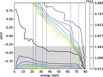
Figure 12. Distribution functions for beam ions in shot 45091 at 0.35 s predicted by ASCOT5 when CX is off (dashed) and when CX is simulated using the best-estimate neutral density profile whose TRANSP part includes recombination atoms (solid), integrated over the spatial domain where R = 1.33–1.60 m and z = −0.10–0.10 m (figure 10). Pitch =  , where
  is the velocity component parallel to the magnetic field line and v is the total speed. Neutral-beam injection energies are indicated using grey dashed lines and the range of initial pitch values using a shaded grey band.
Download figure:
Standard image High-resolution image5. Summary
Based on observations from the first experimental campaign in MAST-U (MU01), CX was suspected to cause significant beam-ion losses, making the device an interesting environment for the study of fast-ion CX. A new model, dubbed BATS1D, was developed to reconstruct the outer-midplane neutral density based on D-alpha measurements carried out using the HOMER camera and Thomson scattering measurements of electron density and temperature. Due to uncertainties in the calibration of the D-alpha measurements, they were scaled based on an extensive comparison of D-alpha measurements and KN1D modelling for experiments in the second MAST-U campaign (MU02). The ability of the ASCOT orbit-following code to simulate beam-ion CX in MAST-U was tested through comparison to MU01 experiments, and the impact of CX on beam-ion confinement was investigated. The fast-ion CX models of ASCOT4 and ASCOT5, both of which were used for analysis, were benchmarked and found to agree, rendering them equivalent in the analysis in this article.
The neutral density reconstruction agrees with SOLPS-ITER modelling for MU01 experiments in terms of the slope of the neutral density profile at the separatrix when plotting on a logarithmic scale, suggesting that the simple BATS1D neutral density model can be used to make physically relevant predictions for the outer midplane in MAST-U. Since beam ions in MAST-U orbit significantly further out in the plasma on the low-field side, especially around the outer midplane, the error introduced by assuming a poloidally uniform neutral density distribution is expected to be significantly mitigated. When fast-ion CX was accounted for in modelling of an MHD-quiescent plasma, predicted neutron emission from the plasma was quantitatively more consistent with fission chamber measurements than when CX was neglected. However, complete quantitative agreement between predicted and measured neutron rates was not achieved, possibly due to remaining errors in the fission chamber calibration. When fast-ion CX was accounted for in simulations using the BATS1D neutral density reconstruction, the measured passive FIDA signal was mostly reproduced both quantitatively and qualitatively. When CX losses were neglected, the measured signal was not reproduced quantitatively or qualitatively. The predicted signal was two to four times as high as the measured signal at low-field-side channels, which is explained by the decrease in the beam-ion density at the plasma edge due to CX losses. Spectra predicted near the edge had proportionally too little highly Doppler-shifted passive FIDA light, which is explained by how particles that should have been quickly lost due to CX were allowed to slow down in the plasma and contribute FIDA light with lower Doppler shift. The results suggest that the BATS1D reconstruction was a good approximation of the outer-midplane neutral density, and indicate that, given an accurate neutral background density, the ASCOT fast-ion CX model is able to predict the impact of CX with edge neutrals on the beam-ion distribution. The results further indicate that CX with edge neutrals has a significant impact on the confinement of beam ions in MAST-U, typically causing a beam power loss of 20% when both beams are on and 40% when only the off-axis beam is on, as well as on their velocity-space distribution near the edge.
A cryoplant will be installed in MAST-U in the near future, and is expected to greatly reduce the background neutral density. Given the width of the fast-ion gyro- and drift orbits in MAST-U, the estimated impact of CX, shown in figure 9, demonstrates a significant expected rise in the fast-ion pressure, and hence plasma performance, in the outer regions of the plasma when the cryoplant is operating. The ability demonstrated in this article to account for CX in fast-ion modelling provides an opportunity for more detailed analysis of the impact of fast-ion-driven mode activity on fast ions. If the impact of CX on the fast-ion distribution is accounted for in FIDASIM or neutron modelling, remaining differences between the synthetic and measured FIDA or neutron signals provide a more accurate measure of the impact of fast-ion-driven modes on fast-ion redistribution and loss. An example of such an opportunity is provided by the time period 0.39–0.41 s in shot 44623, when both beams are on, where a mode excited by the on-axis beam appears to be causing substantial beam-ion losses in addition to the CX losses predicted by modelling, as shown in figure 6.
While the results reported in this article represent a significant step towards validating the ASCOT fast-ion CX model, they are limited and carry uncertainties. Once the necessary experimental data is available, the validation will be verified through more precise and comprehensive studies, e.g. using a database of shots to scan over operational parameters, and the investigation of the impact of CX on fast ions will continue. Furthermore, once the HOMER camera has been calibrated and extra scaling factors are unnecessary, BATS1D will become a generalizable tool that can be used, for example, as a point of comparison for more sophisticated neutral models such as KN1D and SOLPS-ITER. Going forward, as uncertainties are reduced and the neutral background reconstruction is improved, the ability to accurately simulate fast-ion CX will be useful in a wide range of increasingly detailed modelling activities in the endeavour to better understand fast ions in spherical tokamaks and other magnetic-confinement fusion devices. Such activities may be expected to improve confidence in predictions of alpha-particle physics in fusion power plants, particularly with regard to redistribution and loss of these particles due to instabilities and 3D field perturbations.
Acknowledgment
We thank William Heidbrink and Christopher Beckley for helpful discussion. We acknowledge the contributions by Andrew Kirk and Andrew Thornton to the calibration of the fission chamber. The ASCOT simulations were carried out on the EUROfusion High Performance Computer, Marconi-Fusion, at CINECA. We acknowledge the computational resources provided by the Aalto Science-IT project. This work has been carried out within the framework of the EUROfusion Consortium, funded by the European Union via the Euratom Research and Training Programme (Grant Agreement No. 101052200—EUROfusion) and also with support from the EPSRC (Grant No. EP/W006839/1) and the US DoE Grant No. DE-SC0019007. Views and opinions expressed are however those of the author(s) only and do not necessarily reflect those of the European Union or the European Commission. Neither the European Union nor the European Commission can be held responsible for them. This work was partially funded by the Academy of Finland Projects Nos. 324759, 328874 and 353370.
Data availability statement
The data that support the findings of this study are openly available at: https://doi.org/10.14468/sdz4-gv05.
Appendix A: Benchmarking CX in ASCOT4 and ASCOT5
The 5th version of the ASCOT orbit-following code (ASCOT5), which is a complete rewrite in the C programming language for the purpose of taking advantage of the parallelization capabilities of modern supercomputers, has previously been benchmarked against the 4th version (ASCOT4 [4]) without the inclusion of CX reactions [5]. The fast-ion CX model of ASCOT4 has previously been analytically verified, benchmarked against the fast-ion module NUBEAM [7] of the transport code TRANSP [8, 9], and demonstrated as a modelling tool [10]. The same model was adapted to and implemented in ASCOT5. In this section, predictions of the ASCOT5 CX model are benchmarked against those of the ASCOT4 CX model.
This benchmark was performed for MU01 shot number 44623: a double-null H-mode plasma with 750 kA of plasma current and a conventional divertor configuration. The chosen time was at 0.39 s when both the on- and off-axis beams were on. First, a TRANSP simulation was run for this case. The TRANSP run was prepared using the OMFIT program [31] based on experimental data from the MAST-U database. The equilibrium was reconstructed using processed data from the MAST-U database, which in turn was originally calculated using the EFIT++ code [32, 33] using magnetic measurements. An EFIT++ reconstruction constrained by measurements carried out using the motional Stark effect diagnostic was not available. TRANSP recalculates the equilibrium, resulting in minor differences from the original EFIT++ reconstruction, relative differences estimated at 1%. The electron density and temperature profiles were reconstructed based on Thomson scattering data [18] using a fitting tool in OMFIT. The main plasma and beam species was deuterium. A single impurity species was assumed: fully ionized carbon, the plasma having an effective charge state ( ) of 1.5. Both ion temperatures were assumed to be equal to the electron temperature, since the on-axis beam was turned off for most of this shot and there were no useful ion temperature measurement data. The neutral background was assumed to consist purely of deuterium atoms. The atomic density and temperature inside the plasma were calculated using a neutral model in TRANSP, the analytic neutral transport model FRANTIC [34, 35]. In the SOL, TRANSP assumes an atomic temperature of 0 eV and a constant atomic density when calculating the CX reaction probability. The atomic density was assumed to be
  m−3, which is the default value used for MAST-U. A 2D contour designed for use with EFIT++ calculations was used as the first wall.
Inputs for the ASCOT runs were copied over from TRANSP, with a few approximations. TRANSP includes fast ions in its quasi-neutrality condition, while the ASCOT plasma was quasi-neutral with the bulk particles alone, resulting in slightly higher bulk ion densities in ASCOT. Plasma temperatures and densities in ASCOT were assumed to be exponentially decaying in the SOL, such that between the separatrix and  values decrease by a factor of 100. The normalized poloidal flux is defined as
  , where
  is the poloidal flux, and
  and
and  are its values at the magnetic axis and inside the separatrix, respectively. For these benchmark simulations, the TRANSP neutral density was imported into ASCOT. Since ASCOT4 does not support a separate neutral temperature, it was approximated as equal to the ion temperature in both ASCOT4 and ASCOT5. The fast-ion CX process is insensitive to the neutral temperature [10]. For technical reasons, the divertors of the 2D wall were in ASCOT replaced with horizontal wall segments at the divertor openings, as shown in figure 4. Since the detailed deposition of fast ions in the divertor is not investigated, this simplification is inconsequential for the modelling reported in this article.
A population of 7155 beam-ion markers, extracted from the TRANSP run, were simulated, with the CX model turned on, until thermalization in both ASCOT4 and ASCOT5. Thermalization was defined as reaching a kinetic energy equal to 1.5 times the local ion temperature or an energy of 100 eV. The full gyro-orbits of the markers were followed. A time step  s was used, which is 0.3% of the gyro-period at the outer-midplane plasma edge. To account for statistical error, the random seeds for the markers were varied and the simulation for each code version was rerun seven times for a total of eight simulations per code version for the same simulation case.
With eight sets of simulation results per code version, average results were calculated and margins of standard error estimated. ASCOT4 predicts that 0.93 ± 0.01 MW of 2.5 MW, or 37 ± 0.4% of the power in beam particles ionized in the plasma (excludes shine-through) is lost to the wall, 8 ± 0.2% hit the wall as ions and 28 ± 0.5% as neutrals. ASCOT5 predicts that 0.91 ± 0.01 MW of 2.5 MW, or 36 ± 0.4% of the power is lost, 8 ± 0.1% hit the wall as ions and 27 ± 0.4% as neutrals. Separating particles that hit the wall by charge approximates separating orbit and CX losses, but it is not an exact measure. A particle that is lost due to CX may be reionized before it hits the wall. Moreover, a particle born on a loss orbit may be lost through CX before its orbit intersects the wall. In ASCOT4, the average of the median times for beam particles to hit the wall as a neutral is 0.28 ± 0.008 ms after being ionized in the plasma. In ASCOT5, this time is 0.26 ± 0.01 ms. The ASCOT5 results agree with the ASCOT4 results within margins of standard error.
All 16 simulations were also repeated with the CX model turned off to allow direct comparison of the agreement between ASCOT4 and ASCOT5 with and without the inclusion of CX processes. Figure A1 shows the beam-ion content in the plasma as a function of  . Beam-ion content is given as the number of particles in the volume element corresponding to the
  coordinate. Each profile is an average of the predictions from the eight corresponding simulations. The differences between the ASCOT4 and ASCOT5 predictions, with and without CX reactions, are shown on a separate axis. Good agreement is observed in both cases, but there appears to be some systematic discrepancy, with ASCOT5 mostly predicting marginally higher beam-ion content. The difference is larger when CX reactions are included. Omitting only the very core and analysing outside
  , when CX is turned off, the code versions agree to within 2%. When CX is turned on, the code versions agree to within 4%. The reason for the marginal discrepancies is unclear and under investigation. However, the agreement in this comparison is good enough to consider the code versions equivalent on the level of precision featured in the analysis reported in this article.

Figure A1. Simulated beam-ion content in MAST-U shot 44623 at 0.39 s as a function of the normalized poloidal flux  , where
  is the poloidal flux, and
  and
and  are its values at the magnetic axis and inside the separatrix, respectively. Beam-ion content is given as number of particles in the volume corresponding to the
  coordinate. Each profile is an average of the predictions from eight simulations of the same case, differing only in the random seeds of the markers. Relative differences in the profiles from the two ASCOT versions are shown on a separate axis.
Download figure:
Standard image High-resolution imageFigure A2 compares the predicted beam-ion distributions, integrated over the whole spatial domain, as functions of energy and pitch when CX is accounted for. Each distribution is an average of the predictions from the eight corresponding simulations. Good agreement is observed. Noticeable deviations are found only in the bottom right corner where the energy is high and the pitch highly negative, which corresponds to the start of a simulation, i.e. just after a particle has been injected into the plasma. On the far-right, where the largest deviations are, statistics are low.
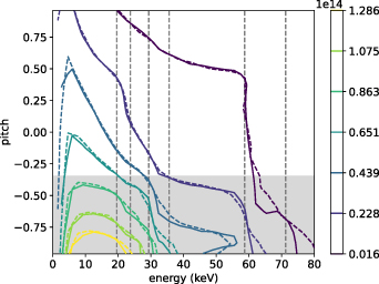
Figure A2. Distribution functions predicted by ASCOT4 (solid) and ASCOT5 (dashed) for beam ions in MAST-U shot 44623 at 0.39 s, integrated over the whole spatial domain. Each distribution is an average of the predictions from eight simulations of the same case, differing only in the random seeds of the markers. Pitch =  , where
  is the velocity component parallel to the magnetic field line and v is the total speed. Neutral-beam injection energies are indicated using grey dashed lines and the range of initial pitch values using a shaded grey band.
Download figure:
Standard image High-resolution imageFigure A3 shows the spectra for the final kinetic energies of markers that hit the wall when CX was accounted for. Each spectrum is an average of the predictions from the eight corresponding simulations. Estimated margins of standard error are shown using shaded colour bands. The predictions by ASCOT4 and ASCOT5 agree within margins of standard error. The six injection energies featured in the two-beam experiment are indicated in the figure. Peaks in the loss spectra correspond to the injection energies. A significant fraction of the losses are direct orbit losses, but most are from CX, as implied by the charge-specific power losses listed above. Peaks in the loss spectra just below the injection energies are expected, since maximal gyroradii maximize the likelihood of orbits intersecting the wall and expose the beam ions to maximal neutral density. Furthermore, beam-ion populations on orbits intersecting the wall and on orbits exposed to high neutral density are quickly depleted, explaining the sharpness of the peaks.

Figure A3. Simulated spectra for the final kinetic energies of beam-particle markers that hit the wall in MAST-U shot 44623 at 0.39 s. Each spectrum is an average of the predictions from eight simulations of the same case, differing only in the random seeds of the markers. The shaded colour bands indicate estimated margins of standard error, with colours matching the corresponding average spectrum. Neutral-beam injection energies are indicated using grey dashed lines.
Download figure:
Standard image High-resolution imageThe two code versions ASCOT4 and ASCOT5 are both used in the analysis reported in this article, with emphasis on the CX models of the code versions. The benchmark reported in this section shows good agreement between the code versions in a range of tests representative of analysis of fast ions in the presence of CX reactions in the MAST-U spherical tokamak. The level of agreement is deemed sufficient to render the code versions equivalent in the analysis in this article.
Appendix B: Working around calibration uncertainties
There was uncertainty in both the spatial and brightness calibrations of the HOMER camera in MAST-U. Therefore, the BATS1D model introduced in section 2.1 could not be directly used. The uncertainties were circumvented with ad hoc solutions to allow progress in reconstructing the neutral density.
There was uncertainty in the accuracy of the major radius coordinate R for the HOMER data, i.e. the tangency radii corresponding to the sightlines of the camera channels. A spatial calibration to check if the real view matches the virtual view in the HOMER CAD (computer-aided design) model had not yet been conducted. However, four alternative mappings of the HOMER channels to tangency radii had been calculated. They all appear misaligned, as they would place the D-alpha peak either deep inside the plasma or far outside the separatrix. In a simple virtual reconstruction of the tokamak, made in Matlab independently of the HOMER CAD model, these candidate abscissae were compared to a design schematic that had been used for the installation of the HOMER camera in the vessel wall. The schematic shows two coordinates for the camera, determining its position and viewing direction in the device. For each of the four candidate abscissae, sightlines from the camera lens to the left-most and right-most tangency points, when viewed from above, were calculated in Matlab. Then the bisector was calculated as an estimate of the central sightline and compared to the central sightline based on the camera schematic. The set of tangency radii whose estimated central sightline best matched the schematic was chosen. The chosen abscissa still placed the D-alpha peak too far outside the plasma. Therefore, the abscissa was shifted such that the D-alpha peak aligned with the separatrix. Details on how this shift was calculated are given below.
Typically, an absolute brightness calibration is applied to the raw HOMER data to translate counts registered by the sensor to power emitted by the plasma. Then the inverse Abel transform is applied to the line-integrated brightness signal to acquire the emissivity as a function of major radius. Finally, the signal is multiplied by 4π sr to account for emission in all directions from a plasma volume element. If BATS1D could be directly applied to the obtained emissivity, this would be the extent of the data processing for the brightness measurement. However, there was uncertainty in the HOMER brightness calibration. Unlike in MU01, in MU02 there was an operational FIG to measure neutral gas pressure at the vessel wall, which allowed the use of KN1D to simulate D-alpha emissivity profiles. Extensive comparison of HOMER measurements and KN1D modelling was performed for MU02 experiments to find a scaling factor to complement the above described typical data processing and raise the D-alpha emissivity obtained from HOMER to a level consistent with KN1D modelling. The configuration of the HOMER camera was the same in MU02 as it had been in MU01.
A number of high-confinement mode (H-mode), low-confinement mode (L-mode) and ohmic MU02 shots and time points were chosen for the study to estimate a scaling factor for the HOMER signal for use in modelling certain MU01 experiments. The aim was to choose MU02 cases similar to the MU01 cases to maximize comparability and, therefore, the physical accuracy of the resulting scaling factor. Several MU02 cases were chosen for each MU01 case, but single, most similar cases were also selected to get case-specific best-estimate scaling factors. Similarity was judged based on plasma scenario, confinement mode, time point during the shot, both line-integrated and full-profile electron density, both core and full-profile electron temperature, fuelling scheme, beam configuration, and line-integrated midplane D-alpha emissivity. Table B1 lists the shot numbers and time points for the 15 chosen cases as well as the relevant results of the study. The H-mode cases were chosen to be similar to the MU01 H-mode case of shot 44623 at times 0.31–0.33 s and 0.39–0.41 s whose neutron emission is investigated in section 3. Across the investigated time periods for shot 44623, the time point 0.32 s, when the plasma is in a relatively steady state, was chosen as the time point for the neutral density reconstruction. Shot 46957 at 0.32 s was selected as the MU02 case most similar to shot 44623 at 0.32 s. The L-mode cases were chosen to be similar to the MU01 L-mode case of shot 45091 at time 0.35 s whose passive FIDA is investigated in section 4. Shot 46618 at 0.22 s was selected as the most similar MU02 case. The ohmic cases were chosen to be similar to the MU01 ohmic case of shot 45469 at time 0.40 s, for which neutral density estimates by BATS1D and SOLPS-ITER are compared in appendix C. Shot 47113 at 0.43 s was selected as the most similar MU02 case.
Table B1. A list of the MU02 cases, in terms of shot number and time point, that were used to determine the distance shift needed to correct the spatial calibration of HOMER and the scaling factor needed to complement the brightness calibration of HOMER. The plasma type is indicated as a confinement mode or heating scheme. The fourth column records the distance shift needed to align the HOMER peak with the separatrix location. The fifth column records the ratio between the KN1D-simulated and HOMER-measured D-alpha peak amplitudes.
| Type | Shot | Time (s) | Shift (m) | Ratio |
|---|---|---|---|---|
| H-mode | 46957 | 0.32 | −0.113 | 5.0 |
| 0.40 | −0.112 | 4.9 | ||
| 47036 | 0.32 | −0.106 | 5.6 | |
| 0.40 | −0.095 | 5.5 | ||
| L-mode | 46618 | 0.20 | −0.135 | 3.4 |
| 0.22 | −0.118 | 4.1 | ||
| 46624 | 0.35 | −0.115 | 4.1 | |
| 0.37 | −0.114 | 5.0 | ||
| 46828 | 0.25 | −0.122 | 3.1 | |
| 46875 | 0.35 | −0.114 | 2.2 | |
| Ohmic | 47113 | 0.35 | −0.112 | 4.1 |
| 0.38 | −0.107 | 3.8 | ||
| 0.43 | −0.108 | 4.8 | ||
| 0.54 | −0.114 | 3.7 | ||
| 47121 | 0.20 | −0.110 | 3.1 |
Before comparing D-alpha profiles from HOMER and KN1D to circumvent the uncertainty in the brightness calibration for HOMER, a distance shift for the HOMER data was estimated to circumvent the uncertainty in the spatial calibration for HOMER. The HOMER camera should not move between experiments, so the error in the spatial calibration should be consistent. Therefore, a single distance shift, to be used for all modelling cases in this article, was estimated as the average of the distance shifts needed to move the Abel-inverted HOMER peak to the separatrix in each of the individual MU02 cases. The HOMER peak location was defined as the midpoint of the full width at 95% of the maximum emissivity. To estimate the major-radius coordinate of the separatrix at the outer midplane,  , the upstream electron temperature at the separatrix,
  , was estimated. To calculate
  , the expected parallel electron heat flux density was integrated along the separatrix derived by EFIT++ (see for example equation (4) in [36]). The
  was then assumed to be where the linearly interpolated Thomson scattering electron temperature profile crosses the estimated
  . When applying this model, the power crossing the separatrix was assumed equal to the ohmic heating power, which causes slight underestimation of
  in the cases with one or two beams. The error introduced by this was estimated for shot 44623 at 0.32 s, where TRANSP predicts 0.7 MW of input ohmic power and 1.5 MW of deposited beam power. In this case, approximating the power crossing the separatrix as equal to the sum of ohmic and beam heating power instead of only ohmic heating power gives a result three times as large. The expected value of
  then becomes
  times as high. This translates into a 3 mm smaller
  . Moreover, the radial decay length for the heat flux in the SOL was assumed to be 10 mm, a common default value based on studies performed for MAST data [37, 38]. The sensitivity of
  on this parameter was tested for shot 46957 at 0.32 s. When the decay length was varied between 5 mm and 15 mm,
  varied between 33 eV and 24 eV, which translates into a variation in
  of 4 mm. The spatial coordinates of the Thomson scattering data at the separatrix are precise to 1 cm. The distance shifts needed to move the Abel-inverted HOMER peak to the separatrix in the investigated MU02 cases are listed in table B1. The average distance shift is −11.3 cm along the major radius and was applied to HOMER data used in modelling in this article. Since the above estimated uncertainty in
  is small compared to the spatial uncertainty in the Thomson scattering data and compared to the variations in the distance shift and D-alpha peak ratio in table B1, error margins are not calculated based on the uncertainty in
  .
.
For each MU02 case, the D-alpha emissivity profile measured by HOMER on the outer midplane was compared to the profile predicted by KN1D. The inputs for the KN1D simulations were the scalar neutral gas pressure measured by the FIG at the vessel wall, time-averaged 10 ms in each direction, as well as the electron density and temperature profiles measured using Thomson scattering. The main result of each comparison is the ratio between the peak values of the KN1D and HOMER D-alpha profiles near the separatrix. The ratios are listed in table B1. The minimum and maximum ratios were 2.2 and 5.6, respectively. These were used as limiting-estimate scaling factors for HOMER D-alpha measurements from MU01, the expectation being that the true D-alpha value is somewhere between the resulting limiting estimates. In addition, best-estimate scaling factors were selected for the different MU01 cases based on their most similar MU02 counterparts, which were listed above. The best-estimate scaling factor for shot 44623 at times 0.31–0.33 s and 0.39–0.41 s is 5.0, for shot 45091 at time 0.35 s it is 4.1, and for shot 45469 at time 0.40 s it is 4.8.
The calculated ratios between D-alpha peaks do not reflect possible mismatch in the exact peak locations, but it was confirmed that HOMER and KN1D are in reasonable agreement about the peak locations along the major radius. Using the same definition as above for a D-alpha peak location, the two peaks were within 2 cm both of each other and of the separatrix estimate in all 15 cases. In 12 cases, the peaks were within 1 cm of each other and the separatrix. These observations imply that the distance shift calculated for and applied to the HOMER data, −11.3 cm, is a successful shifting correction to the error in the spatial calibration. However, a possible error in the spacing between the HOMER R points is not corrected by the shift. Indeed, when comparing HOMER and KN1D D-alpha profiles, it was observed that the HOMER peak tended to be wider, which could be explained by an overestimation of the spacing between the HOMER sightlines.
The KN1D prediction of D-alpha emissivity only considers atoms. As discussed in section 2.1, molecules contribute to D-alpha as well, and the HOMER measurement is expected to include this. However, based on the KN1D modelling, and the SOLPS-ITER modelling discussed more in appendix C, atomic density is typically about an order of magnitude higher than molecular density at the separatrix. In the SOL, the molecular density typically becomes higher than the atomic density within a few centimetres of the separatrix and settles at a level about an order of magnitude higher than the atomic density. Since the scaling factors calculated for the HOMER emissivity signal are based on the D-alpha peaks at the separatrix, error from the omission of D-alpha from molecules in KN1D is expected to be low. What error there is will lead to an underestimation of the total neutral density and its impact on fast ions, as far as this part of the reconstruction is concerned. Since the whole HOMER D-alpha emissivity profile is scaled based on the peak ratio at the separatrix, a molecular contribution to the HOMER profile in the shape of a thicker tail in the SOL will be included. However, the signal drops rapidly in the SOL with the drop of the electron density. The reconstruction of the neutral density in the SOL is further discussed in section 2.2. A molecular contribution is a second possible explanation for why the HOMER peaks tend to be wider in the SOL than the KN1D peaks. CX losses of fast ions due to interaction with molecules are further underestimated since the molecular density that is accounted for is approximated as additional atomic density. The models for the neutral background in ASCOT4 and ASCOT5 are currently limited to atoms, for which the CX reaction probability is modestly lower than for molecules, as was explained in section 2.1.
When comparing HOMER and KN1D D-alpha profiles, two additional noteworthy observations were made. Looking carefully at the beam timings and comparing the HOMER D-alpha from the different MU02 cases, there is evidence that the interaction between beam particles, especially those from the off-axis beam, and background neutrals generates enough additional D-alpha to significantly inflate the D-alpha peak measured by HOMER, both in height and in width. The transmission function for the wavelength filter of HOMER is approximately a Gaussian where the central wavelength is 655 nm and the full width at half maximum is 10 nm, which means that Doppler-shifted fast-ion D-alpha is not excluded. Hence, a beam-ion contribution is indeed expected in the HOMER measurement. KN1D does not simulate any fast-ion contribution. Therefore, this is a third possible explanation for why the HOMER D-alpha peak tends to be wider than the KN1D peak. This could also explain the higher peak ratios obtained for H-mode compared to L-mode, as shown in table B1, since the fast ions make a larger relative contribution in L-mode where the bulk density is lower at the edge. However, it should be noted that the ohmic cases, where there is no beam-ion contribution, also yield lower ratios than the H-mode cases. An impact by beam particles was observed also in the line-integrated midplane D-alpha measurements. The other noteworthy observation is that measurement noise in the SOL electron density and temperature from Thomson scattering, which was allowed to propagate through to the KN1D inputs, can cause KN1D to predict significant D-alpha in the SOL, which, in turn, results in a lower peak at the separatrix. This could cause KN1D to underestimate the D-alpha peak at the separatrix.
There are a number of details about the Thomson scattering and HOMER data used in this work that were not mentioned above but should be noted. In all the analysis done related to reconstructing the neutral background, HOMER brightness data were time-averaged 10 ms in each direction, and Thomson scattering electron density and temperature data were time-averaged 20 ms in each direction. Thomson scattering data points were considered spurious and filtered out if they had a value more than twice the value of the previous point when moving radially outward along the outer midplane. Beyond this, noise in the Thomson scattering measurements, which is substantial especially in the SOL, was allowed to propagate through to the neutral density calculations. The used Thomson scattering data were interpolated at the HOMER R abscissa, which has significantly higher spatial resolution, for the final insertion into the inverted KN1D equations. The HOMER camera is located 18.3 cm above the midplane. This is significant since the separatrices of equilibria in MU01 and MU02 plasmas tend to have a bulge at the outer midplane. The value of the separatrix R coordinate on the HOMER plane is typically 2–3 cm smaller than on the Thomson scattering plane, which is 1.5 cm above the midplane, i.e. essentially on the midplane. This vertical misalignment of the HOMER and Thomson scattering sightlines was accounted for by mapping the R coordinates from the HOMER plane via the flux coordinate  , which was based on an EFIT++ equilibrium reconstruction, to the Thomson scattering plane. This mapping was performed in the opposite direction for the separatrix location, which was calculated based on Thomson scattering data, when it was compared to the HOMER peak location to calculate the distance by which to shift HOMER data.
Appendix C: Comparing to SOLPS-ITER
To test the BATS1D model for neutral density reconstruction, including the extra corrections described in appendix B, it was compared to SOLPS-ITER modelling performed for ohmic L-mode shots from MU01 [19]. The case modelled in SOLPS-ITER was a double-null L-mode shot with a toroidal magnetic field strength of 0.5 T on the magnetic axis, a plasma current of 650 kA and ohmic heating of 0.6 MW. Fuelling was done from the high-field side, and the outer-midplane separatrix density was  m−3, corresponding to a fairly high-density L-mode from MU01. The SOLPS-ITER simulations are 2D in the poloidal plane, with the grid based on the full equilibrium reconstruction by EFIT++. The SOL plasma is modelled as a fluid while the neutrals are modelled kinetically. Various neutral reactions are considered, including recycled molecules and their breakup. The model is considerably more complete than BATS1D and, therefore, serves as a good benchmark. However, due to the lack of pressure gauges in MU01, the SOLPS-ITER modelling is not experimentally constrained and the absolute values of the neutral densities predicted cannot be assumed physically accurate. In that sense, the BATS1D modelling for MU01 is more experimentally relevant, since the D-alpha profile is scaled based on KN1D modelling constrained by pressure measurements from MU02. It is more useful here to compare BATS1D to SOLPS-ITER in terms of the shape of the neutral density profile rather than its magnitude.
One of the plasmas on which the SOLPS-ITER modelling is based, and the one chosen to be modelled using BATS1D for this comparison, is MU01 shot 45469 in the time period 0.25–0.75 s. Instead of simulating a single time point, SOLPS-ITER runs to steady state. For the BATS1D modelling, the time 0.40 s was chosen because of the relatively steady state of the plasma. Figure 3 shows the data that BATS1D uses to estimate the neutral density: the outer-midplane Thomson scattering electron density and temperature data as well as the HOMER signal that has been absolutely calibrated, Abel-inverted, shifted, mapped to the Thomson scattering plane and scaled to complement the uncertain absolute calibration. From a set of SOLPS-ITER simulations where the assumed fuelling rate was varied, that case was chosen whose electron density at the outer-midplane separatrix best matches the Thomson scattering measurement for shot 45469 at 0.40 s.
The BATS1D and SOLPS-ITER neutral density estimates near the outer-midplane separatrix are shown in figure C1. SOLPS-ITER estimates both the atomic and molecular deuterium densities. Both the separate profiles and the total neutral density are shown. As explained in appendix B, BATS1D, scaled based on KN1D modelling for MU02, includes molecules a limited distance into the SOL if the molecular density at the separatrix is small, which SOLPS-ITER suggests it is in this case. Therefore, the BATS1D result should be interpreted as a total neutral density and compared to the total neutral density estimate by SOLPS-ITER. The BATS1D estimate, even its upper limit, is significantly lower than the SOLPS-ITER estimate, by a factor of two or more at the separatrix. The Thomson scattering noise plays a large role in the shape and maximum value of the BATS1D profile outside the separatrix. In the range 4–5 cm outside the separatrix, the difference between the BATS1D and SOLPS-ITER estimates approaches an order of magnitude, but in the range 5–6 cm there is a sharp increase in the BATS1D profile, which returns the difference to about a factor of two. Further out, the BATS1D profile starts dropping with the electron density. As explained, the SOLPS-ITER modelling is not experimentally constrained and could be overestimating the neutral density. A more useful comparison to make is that of the profile slopes. When plotted on a logarithmic scale, the slope of the BATS1D neutral density profiles agrees with that of SOLPS-ITER at the separatrix, and a few centimetres into the plasma. This implies that the BATS1D model is able to correctly capture the steep gradient of the neutral density at the outer-midplane separatrix in a MAST-U plasma. Deeper inside, the BATS1D slope levels out while that of SOLPS-ITER remains steep. This implies that the BATS1D profile becomes unreliable deeper inside the plasma. This may be explained by how the edge is very bright, but little D-alpha from deeper inside the plasma reaches the HOMER lens. Via an imperfect Abel-inversion of the line-integrated brightness, the neutral density may then be overestimated deeper inside the plasma. This observation is taken into account in section 2.2 when constructing the full neutral density profiles to be used in ASCOT and other modelling.
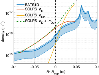
Figure C1. Estimates by BATS1D and SOLPS-ITER of the outer-midplane neutral deuterium density near the separatrix in shot 45469 at 0.40 s as a function of major radius minus the major-radius coordinate of the separatrix. For SOLPS-ITER, atomic ( ) and molecular (
 ) densities are also shown separately. For BATS1D, the result when scaling with the best-estimate scaling factor for this case, 4.8, is shown using a solid blue line. The results using the minimum and maximum scaling factors, 2.2 and 5.6, respectively, are indicated using a shaded blue band.
Download figure:
Standard image High-resolution image