
Abstract
An effort to achieve high-energetic ion beams from the interaction of ultrashort laser pulses with a plasma, volumetric acceleration mechanisms beyond target normal sheath acceleration have gained attention. A relativistically intense laser can turn a near critical density plasma slowly transparent, facilitating a synchronized acceleration of ions at the moving relativistic critical density front. While simulations promise extremely high ion energies in this regime, the challenge resides in the realization of a synchronized movement of the ultra-relativistic laser pulse ( 30) driven reflective relativistic electron front and the fastest ions, which imposes a narrow parameter range on the laser and plasma parameters. We present an analytic model for the relevant processes, confirmed by a broad parameter simulation study in 1D- and 3D-geometry. By tailoring the pulse length and plasma density profiles at the front side, we can optimize the proton acceleration performance and extend the regions in parameter space of efficient ion acceleration at the relativistic density surface.
Export citation and abstract BibTeX RIS

Original content from this work may be used under the terms of the Creative Commons Attribution 4.0 license. Any further distribution of this work must maintain attribution to the author(s) and the title of the work, journal citation and DOI.
The acceleration of ions using lasers has great potential for breakthrough applications, which require short pulse durations, high currents, high emittances or a small accelerator footprint [1–3]. One of the most widely used performance benchmarks in practice is the maximum achievable ion energy. In the pursuit for higher maximum ion energies, progress has been made with more powerful petawatt lasers [4, 5], controlled pulse delivery [6–9] and optimized targets [10–12]. Over the last two decades, the field has witnessed an improvement of the maximum proton energy from  , obtained early in 1999 [13], to recently more than
  [14, 15]. Despite the theoretical and experimental understanding that enabled the optimization of laser ion acceleration in recent years, it is still a long path towards the
  –
– required to enable applications such as tumour therapy [1, 16, 17].
The above cited experiments [14, 15] were performed on relatively long pulse lasers with up to half a picosecond pulse duration. Those lasers are limited to low repetition rates, while ultra-short pulse lasers in the few tens of femtoseconds range can operate in the  regime and are also more favourable due to reduced costs. Most notably, these machines can now be operated in a very reproducible and reliable fashion, such that, over a timespan of several months, protons with
  can be generated routinely [8].
It is notable that virtually all experiments that report high proton energies were employing one variant of the established target normal sheath acceleration (TNSA) [18–20] or transparency enhanced TNSA method [21–24]. Hence, it is clear that in order to soon reach the envisioned  or more, breakthrough innovations are needed. The electrons act as a mediating medium in the energy transfer process between the laser and the ions and thus mitigate the potential efficiency of the whole acceleration process. One major drawback of TNSA is that the ions from the solid target rear surface are accelerated indirectly via the electrons by expansion of the plasma anode. As a consequence, the light protons only briefly experience the maximum possible acceleration field at the rear surface before they detach from the bulk, the target surface degrades, and the electron sheath explodes transversely. Candidates to overcome this limitation are collisionless shock acceleration and radiation pressure acceleration (RPA). There, the laser pushes an electron sheath in front of the ions. This can happen either at the front surface of a foil (hole boring RPA, HB-RPA [25, 26]) or it pushes forwards all electrons of a very thin foil. In the latter case, the laser pressure continuously accelerates the whole foil and hence the ions (light sail RPA, LS-RPA [27, 28]). However, transverse instabilities and subsequent plasma heating pose practical limitations on the acceleration of ions to high energies, which are challenging to overcome [29, 30].
Another particularly interesting alternative is near critical density targets, e.g., hydrogen jet targets. These target systems can provide for cylindrical and planar micron-sized geometry and virtually debris-free high repetition rate operation [31, 32]. One theoretical mechanism of continuous and direct energy transfer from the laser to ions is a form of relativistic hole boring: Instead of boring into the plasma, the laser now penetrates into the relativistically transparent plasma as it pushes forward the relativistic critical density front, synchronized to the acceleration of ions. This is the mechanism of 'synchronized acceleration of ions using slow light' described in [33–37]. However, the naming can be confusing as the core of the mechanism is not the change of the propagation velocity of the laser light inside the plasma but rather the fact that the point of laser reflection, i.e. where the ions are accelerated, penetrates slowly into the plasma.
The laser penetration happens progressively as the laser turns the plasma partially transparent at the front, by virtue of relativistic mass increase in the electrons oscillating (linear polarization) or circulating (circular polarization) in the intense laser field. The front that separates the relativistically transparent region from the opaque plasma with a density above the relativistic critical density (below referred to as 'relativistic transparency front', RTF) moves forward slowly (compared to the speed of light) and accelerates as the laser intensity increases, which gives the ions time to accelerate and follow it in a synchronized fashion. The acceleration force is generated via the charge separation field induced by the laser pressure at the front.
In this respect, this mechanism is similar to hole boring RPA, only here instead of the critical density surface at the target front the radiation pressure is now exerted at the RTF inside the plasma. Therefore, we call this process RTF-RPA throughout this paper. Generally, the velocity at which the laser bores into the plasma depends on the plasma density and laser intensity; the equilibrium RTF velocity increases with intensity and the decreasing electron density [38]. Simulations can demonstrate that in the optimal case when the laser acceleration of the RTF is synchronized to the ion acceleration, the ion energy can be dramatically increased compared to, e.g. hole-boring or TNSA [33–37].
Here, we develop a self-consistent semi-analytic model to calculate the maximum ion energies in the RTF-RPA regime and use this to infer optima for the laser pulse duration and plasma density profile.
1. RTF-RPA mechanism
Before we introduce the semi-analytic model, we briefly review the RTF-RPA mechanism. Figure 1 shows a schematic picture of RTF-RPA. The laser penetrates the plasma with a free electron density ne
, accelerating or heating them at the front, thereby increasing the critical density  . At the RTF (
 ) the laser is reflected and a charge separation field accelerates the ions. As mentioned above, RTF-RPA shares certain similarities with hole boring: The reflective surface where
  is pushed forward and ions are reflected at the moving surface. The characteristic difference is that with RTF-RPA it is not the plasma material n0 itself that is pushed forward but the reflective surface moves via a progressive increase of γ. In this case, the penetration velocity is accelerating much faster with an increase of the laser intensity so that the front can keep up with the reflected ions. Perfect synchronization is not required, as long as the RTF is accelerated fast enough for the ions to be caught up and accelerated repeatedly.
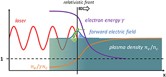
Figure 1. Schematics of the RTF-RPA mechanism.
Download figure:
Standard image High-resolution imageIn figure 2 we exemplify this for an intense laser with  , linear polarization P = 1, and
  FWHM pulse duration for a Gaussian temporal intensity profile
  . The plasma density was optimized w.r.t. maximum ion energy gain by RTF-RPA to
  in a 1D geometry SMILEI [39] simulation. Since RTF-RPA is essentially a 1D process, we expect the 1D simulations and a 1D model to capture the essential physics. Later, we will compare our results also to 3D simulations, which indeed show the same characteristic features and trends.

Figure 2. Velocity (a) and position (b) of the relativistic density front and highest energy ions as function of time. (c) The electric field (top), maximum ion energy (centre) and densities (bottom) for two timesteps during the RTF-RPA process, the position of the relativistic density front is marked by the blue vertical line. (d) Proton spectrum at the end of the simulation. Simulation parameters: see main text.
Download figure:
Standard image High-resolution imageThe simulated plasma consists of free protons and electrons. It starts at  from the left simulation box boundary and extends through the whole box to the right boundary. The simulation duration and box size were chosen so that the laser while it is being reflected and the fastest electrons traveling at speed of light do not reach the right box boundary, thereby ignoring any effects a rear surface might induce. The resolution was set to
  . Here and in the following, we use the conventional dimensionless quantities by setting
  . For simplicity we show our results in SI units, where we assumed
  . The full simulation parameters as well as all relevant scripts necessary to reproduce the results is available online [40].
One can see the RTF-RPA mechanism accelerating ions to very high energies. Panels (a) and (b) show the position and velocity of the fastest ion (blue) and of the laser reflection (RTF, orange), respectively. As a reference, in panel (b) we also plot the position of the (non-relativistic) critical density surface (green). While the latter can be seen to move only slowly as a result of the radiation pressure, the point of reflection quickly penetrates due to relativistic transparency into the plasma, in sync with the fastest ions. Even though initially the ions are accelerating slower than the RTF, later the RTF accelerates slowly enough so that the ions start to catch up and co-move with the accelerating field essentially during the whole laser upward ramp. The density and field distribution are shown in (c). In the lower panel, the electron, ion and relativistically corrected electron density profiles  ,
,  ,
,  are plotted normalized to
  for two times, 20 fs and 50 fs after the laser maximum arrival at the target front. The laser is seen to penetrate into the plasma, where it is reflected at the point where the relativistically corrected density surpasses the critical density
  . This point is marked by a blue vertical bar also in the middle and top insets, that show the maximum ion energy profile and electric field profiles respectively. The longitudinal electric field profile shows a distinct peak around the laser reflection point due to the charge separation, and the position of the maximum ion energy coincides with that position. Specifically, for a plasma density of
  , the RTF-RPA process works best for the specific laser pulse duration and peak intensity of the simulation shown in figure 2, where the most energetic ions can co-move with the RTF almost during the whole laser pulse duration. The protons eventually reach a maximum kinetic energy exceeding
  , compared to only
  expected for relativistic hole boring [26].
In fact, hole boring is observed for higher plasma density, as will later be shown in the context of figures 4 and 9(c). For lower densities, the plasma is transparent and the laser-induced charge separation field only sweeps briefly over the ions. Consequently, the ion energy drops dramatically, rendering the energy gain negligible in this regime. For even smaller plasma density or at high values of a0, another regime of efficient ion acceleration in a plasma wakefield is predicted [41, 42], which is beyond the scope of this paper, though it becomes visible at the lowest densities and highest laser intensity shown later in figure 4. We note that the absolute ion energy in the RTF-RPA observed in our simulations is in good agreement with the results in [33], where for the same laser parameters a 3D simulation has shown proton acceleration in a  foil to
  by RTF-RPA, albeit at somewhat higher density of
  [43].
[43].
The underlying ultimate limitation for the maximum ion energy at a given pulse duration and peak intensity is the coupling of two variables with the one parameter of plasma density: RTF acceleration and maximum RTF velocity. The former needs to be matched to that of the ions so that they can stay close to the RTF, and the latter should be as high as possible as it dictates the maximum possible ion energy limit. The optimum plasma density consequently resembles a compromise between those two optimization goals, since an increase of the RTF velocity would inevitably leave the ions behind during the initial acceleration phase.
2. Results
In order to increase the ion energies achievable with RTF-RPA, ideally one would like to reduce the plasma density in order to increase the terminal RTF velocity, while at the same time keeping the acceleration slow and synchronized to the ions. There are two principal routes to achieve this goal: modifying the pulse shape or modifying the plasma density. We will first examine how a simple laser pulse duration and density variation can optimize the ion energies for a given laser intensity, and then optimize the ion acceleration by introducing a compression layer in front of the plasma. Its dramatic effects of increase of the maximum ion energy and larger range of lower laser intensities where RTF-RPA can still be active are the main findings of this paper.
2.1. RTF-RPA analytic model
Before looking at the details of the simulation results, we briefly review the one-dimensional RTF-RPA process. For small values of a0 the laser pushes forward the front surface via HB-RPA. For larger a0 the laser can penetrate into the plasma by turning the plasma relativistically transparent at the front. The velocity of the point of reflection of the laser can be modelled by:
where  is the HB velocity with
  [26], and

is the velocity of the relativistic critical density front with
and  [38]. The lower subscript f refers to quantities of the RTF where the laser is reflected. The coefficient P refers to the polarization, see below. The plasma is assumed to be homogeneous with electron density
  . Here, we introduced the empiric factor P to approximate the acceleration of the front velocity for both linear laser polarization (P = 1) and circular polarized light (P = 2). For circular polarized light equations (2) and (3) were found to be in good agreement with numerical simulations [38]. Here, we find that also for linear polarization we obtain a good agreement of the model with our simulations when introducing the factor P, cp. figure 2 [44]. For
  the above equation can be approximated to the simple form [38]:
For the case shown in figure 2 with  and
and  the predicted velocity of the RTF from equation (2) is
  , which compares well to a maximum value of
  in the simulation.
Upon laser reflection a charge separation field is set up at the RTF which can reflect downstream ions with peak field strength [38]
While the laser pulse intensity ramps up, the velocity at which the laser turns the plasma transparent increases, i.e. the RTF accelerates and can catch up with the ions. The charge separation field at the front then reflects and further accelerates them repeatedly.
We now combine the above in order to obtain an analytic closed description of the RTF-RPA process in 1D. The acceleration of the ions  during the laser pulse irradiation can be calculated from the usual HB velocity as long as
  , and later for larger laser strengths
  by the equation of motion (EOM) with:
We approximate Ex
to be spatially constant around the front position,  if
if  , and
, and  otherwise. We find empirically from our simulations shown below that the characteristic length L over which the accelerating field extends can be well approximated by a quarter plasma wavelength in the upstream region,

where  is the average Lorentz factor of the electrons in the upstream region.
The EOM can be easily integrated numerically to obtain the ion velocity and energy. For example, we can derive the optimal values for the pulse duration, density or laser amplitude with respect to the final ion energy, see the following sections.
In the optimum case with the maximum ion energy for a given laser, the EOM can easily be integrated analytically. The maximum possible ion energy is dictated by the maximum velocity of the RTF  , which is a function of a0 and
  . The local optimum pulse durations and plasma densities are given when the accelerated ions are reflected the last time exactly when the laser maximum reaches the RTF. Then, they whiteness the full electrostatic potential around the RTF at its maximum strength.
For these optimum cases we start integrating the EOM after the ions have obtained the maximum RTF velocity with respective energy  ,
,  . We make a variable transformation:
and then integrate from  to
to  . We assume
  is constant to first order around the laser maximum during the short post-acceleration phase. After some algebra we obtain:
with  . The optimum maximum energies of protons are plotted in figure 3 as a function of laser strength a0 and plasma density n0.
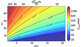
Figure 3. Maximum proton energies as a function of plasma density and laser strength obtained from equation (9) for P = 1 and  . The top axis shows the corresponding
  from equation (10) (i.e. the detailed numerical integration of the EOM (6) in figure 4). The respective laser pulse energy densities
  are shown by iso-contour lines for reference.
Download figure:
Standard image High-resolution image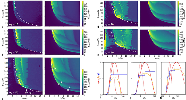
Figure 4. Maximum proton energies as a function of pulse duration  and plasma density n0 for a Gaussian laser pulse temporal profile and homogeneous density n0. Numerical integration of the semi-analytical model on the right, SMILEI 1d simulations on the left. White dashed lines mark the optimum calculated with the semi-analytical model. Panels (f)–(h) correspond to the stars in ((c), right) and show the velocity of the front (orange) and fastest ions (blue), and the normalized laser field strength
  (red, dashed) and
  (red, solid).
Download figure:
Standard image High-resolution imageGenerally, the final ion energy is sensitive to the exact position in the longitudinal field behind the RTF at the time of the laser peak arrival. In these cases, the EOM needs to be integrated numerically piecewise for each reflection in order to obtain the position of the fastest ions in the charge separation sheath.
2.2. Optimum pulse duration
The pulse duration at which RTF-RPA works is a function of laser amplitude a0 and plasma density n0. For laser pulses too short, the ions cannot keep up during the ramp-up, for pulses too long the ions energy will depend on the exact timing of the RTF dynamics and ion acceleration dynamics. To find the optimum pulse duration for specific values of a0 and plasma density n0, we selected five exemplary values for a0 and varied the plasma density and laser pulse duration. For each set, we integrate the EOM and obtain the final hydrogen kinetic energy, shown in the right columns of figures 4(a)–(e). Above, in figure 2, we have shown a simulation for  and
and  . Intuitively, at constant a0 one would expect the ion energy to increase for smaller plasma densities, since the laser front can then propagate faster and the co-moving ions reach a higher final energy. What we find from the numerical solutions of the EOM is in fact such an increase, but only for the envelope along the line of the respective optimum pulse durations. Only at certain values of the plasma density the highest ion energies expected from equation (9) are obtained. These local maxima resemble those optimum conditions when the ions are reflected exactly at the time when the laser maximum reaches the RTF and for which equation (9) was derived. This can be seen in panels (f)–(h). In panel (f) the ion are only reflected once, but the density is smaller than optimum so that the ions are reflected before the laser maximum is reached. Panels (g) and (h) show the respective optimum cases for two and three reflections. Hence, each leaf-shaped area in the
  -space corresponds to a specific number of reflections. When the reflection occurs exactly at the laser maximum arrival, the local optima in the respective leaf w.r.t. ion maximum energy is observed.
To confirm these results we performed a series of 1D PIC simulations with varying initial plasma densities and pulse durations at different peak laser strengths. The results are plotted in figure 4 for the different laser strengths. We extracted the proton energies at  after laser peak arrival on target, when the laser pulse has passed. For a fixed pulse duration, in our parameter range the maximum proton energies due to RTF-RPA are generally obtained at the respective smallest plasma density at which RTF-RPA is still active (onset of RTF-RPA and white dash lines). Only at the highest simulated laser strength we observe similarly high ion energies by ion wave breaking [41, 42]) at smaller density, which is beyond the scope of this paper. The optimum combination of pulse duration and plasma density does not change much with laser strength. It roughly follows the empiric conjecture:

and is in very good agreement with the semi-analytic model, despite its simplistic assumptions. The exact position of the local optimum along the line given by this equation is quite sensitive to the exact timing of when the ions are reflected the last time, which translates into narrow regions of high proton energy.
One can combine equations (9) and (10) to obtain the maximum ion energy as a function of a0 and  , cp. Figure 3 top horizontal axis. In the range between
  and
and  one obtains the approximate scaling of
  at constant tFWHM
. We can also evaluate the maximum ion energy as a function of laser pulse energy density (i.e.
at constant tFWHM
. We can also evaluate the maximum ion energy as a function of laser pulse energy density (i.e.  ), as indicated by the solid lines in figure 3. For a given fixed laser pulse energy density between 0.5 and
  we find that the maximum possible ion energy is expected to be approximately independent of the laser intensity and pulse duration. In figure 5 the results of the numeric integration of the EOM are shown for constant laser pulse energy density matching that of the reference simulation in figure 2 (
 ) and one can readily see that in deed the optimum maximum ion energies at the local maxima do not change much with the pulse duration. For much larger laser pulse energies longer pulse durations would be favoured while for much smaller energies shorter pulse durations are more favourable.
Figure 5. Semi-analytical model: proton energy as a function of plasma density and laser pulse duration for constant pulse energy, equal to that used in figure 2. The leaves clearly each maximize the energy at the same proton energy level, hence the maximum proton energy has no significant dependence on pulse duration.
Download figure:
Standard image High-resolution imageHowever, for very short pulse durations the synchronization between ions and the laser needs to be increasingly more precise, because the difference between too fast laser propagation (ions are left behind early in the laser upramp) and too slow laser propagation (ions are pushed too far ahead and the laser cannot catch up during the short pulse duration) becomes progressively smaller. This means, that in practice the parameter range where RTF-RPA is accessible gets progressively smaller and in the simulations RTF-RPA does effectively not occur for short pulse durations or low laser intensities. Instead, at the predicted optimum RTF-RPA condition we observe a direct transition between transparency and hole boring, with no RTF-RPA in between. The threshold pulse duration below which no RTF-RPA can be observed in the simulations increases with decreasing laser strength. While for  we can observe RTF-RPA down to almost
  , for
, for  we can only see it down to
  .
.
On the other hand, for longer pulse durations the density range at which we observe RTF-RPA increases due to the fact that the ions are pushed forward and reflected at the accelerating RTF multiple times. Slower laser intensity ramp-up in principle simply results in more reflections until the final energy is reached. Additionally, the maximum ion energy becomes less sensitive to the exact timing of the last reflection due to the temporally spread out maximum of the laser intensity and front velocity. Hence, it follows that the higher ion energies occurring at smaller plasma densities due to faster laser penetration require an increasingly longer pulse duration and hence higher laser pulse energy in order for the ions to keep up with the RTF. However, at the longest pulse durations we observe considerable density steepening by the laser pulse at the front, which slows down the acceleration of the RTF. This leads to a dephasing of the laser with the ions and inhibits the synchronization with the acceleration ions eventually. We performed an extensive simulation study testing negative density gradients to circumvent this problem, but due to a very unstable, unpredictive onset of the steepening the synchronization is very delicate between steepening and transparency—, practically, we could not achieve it in our simulations for long pulse durations.
In practice, this means that RTF-RPA is limited both for small as well as high laser pulse energies, which poses an ultimate limit to equation (9) and the maximum achievable ion energy. We can therefore expect the existence of an optimum pulse duration. In the simulations this occurs at the parameter combination at which the second or third ion reflection happens at the laser pulse maximum. In this sense, the case shown in figure 2 hence already resembles a close-to-optimum scenario for a Gaussian beam profile at the given pulse energy density.
2.3. Optimum density compression layer
In order to go circumvent the limits set by hole boring and plasma density steepening on the feasible laser pulse durations, we need another approach to reach smaller plasma densities than just increasing the laser pulse duration. We propose an inhomogeneous target plasma density to match the velocity of the RTF to that of the accelerating ions. A higher density at the target front is employed to achieve this goal by slowing the laser penetration during the initial phase. Specifically, in the following we study a two-layer target consisting of a thin dense front compression layer and a low-density bulk rear. The goal is to set the bulk density to a much lower density than the optimum RTF-RPA density of a homogeneous density to facilitate a high terminal velocity of the RTF. The injection problem, i.e., acceleration rate matching of the ions, is managed by the dense front layer. Experimentally, such a front layer could, for example, be realized by dedicated laser prepulse compression or a tailored laser pulse rising edge contrast profile. Since this compression layer is of higher density than the remaining bulk, the laser needs some time to bore through. This gives the ions enough time for the initial acceleration and to later keep up with the RTF once the laser bores through the front layer. Then, the RTF accelerates further to the final velocity in the less dense rear and—for the same laser parameters—the comoving ions should reach much higher energies than in the case of the respective optimum density homogeneous plasma.
The effectiveness of this method is summarized in a parameter scan in figure 6, again for the same laser parameters as in figure 2 with  and
and  FWHM pulse duration. For a series of 1D PIC simulations of a plasma consisting purely of electrons and protons, we plot the maximum proton energy for different combinations of the front layer thickness and rear layer density. For panels (a), (b), (c) we defined the front compression layer density
  , 28, 56, respectively. For finite values of the front layer thickness we find that the optimum density n0 gets reduced. The optimum front layer thickness is shown by the white dashed lines, as calculated by numerically solving the EOM including the two stages of RTF-RPA first in the dense and secondly in the less dense plasma. It is again in good agreement with the simulations. The larger the front layer thickness d and density n1, the larger is the reduction of the optimum n0 for a given a0. At the same time, we can observe a substantial increase in ion maximum energy, as predicted. For fixed laser intensity and pulse duration the optimum two-layer plasma profile is found at
  ,
,  ,
,  . Then, the maximum ion energy jumps to approximately
  , which is twice the energy of the optimum at homogeneous plasma density using the same laser parameters.

Figure 6. Maximum proton energy after the acceleration process for laser strength  as a function of rear layer density n0 and front layer thickness d for front layer density
  (from left to right). The predictions of the semi-analytic model for the onset of RTF-RPA are indicated by the white dashed lines.
Download figure:
Standard image High-resolution imageThe reason for this large increase in ion energy lies in the higher terminal laser group velocity in less dense plasmas as before, but in this case there is no need for compensation by a longer pulse duration to facilitate more ion reflections. Instead, direct synchronization is achieved by the optimization of the plasma density profile. The ions can be synchronized at lower bulk density at a given short pulse duration, circumventing the limitation by dephasing due to pulse steepening at long pulse duration. Figure 7 shows the dynamics for the optimized two-layer RTF-RPA case. It can be seen that the front velocity reaches a maximum value exceeding  (cf
(cf  , equation (2)), which compares to only
  in the optimum homogeneous density case, see figure 2. Again, panels (b) and (c) show the same characteristic dynamics as before: the most energetic ions comove with the point of laser reflection, which is located inside the plasma where the relativistically corrected electron density surpasses the critical density and a charge separation is induced. Note that now that the laser penetrates the plasma much faster and hence the ion acceleration lasts much longer than before for the optimum case of a homogeneous plasma density in figure 2. While at 50 fs after the laser maximum arrival the ion energy is approximately equal to that of the optimum homogenous density case, in the following 100 fs the ions now continue to be accelerated up to 800 MeV.
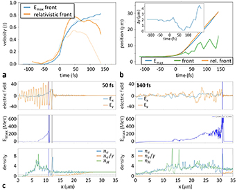
Figure 7. Plasma dynamics for the optimum front layer configuration at  ,
,  ,
,  ,
,  . Light colors in panel (a) show the optimum case without compression layer d = 0 from figure 2.
Download figure:
Standard image High-resolution imageWhat is left is a discussion how exactly the highest energy ions are injected and trapped in the fast moving charge separation field at RTF. The proton phase space is shown in figure 8(a) for several timesteps before and during the RTF-RPA process for the case of optimum ion acceleration with a front compression layer, see figure 7. For comparison, we also show the accelerating electric fields and electron densities in panels (b) and (c), respectively. In panel (c), we scaled the density for each timestep individually for clarity, the thin dashed lines show the respective critical density  for reference. The ion acceleration starts early, already at 40 fs before the maximum arrival the ion gain energy at the front surface, while the electron density
  is still seen to be quite similar to
  . In this phase the laser pushes the surface forward while not yet being intense enough to accelerate electrons to relativistic energies. This changes at around 20 fs before the laser pulse maximum arrival. Now the laser penetrates into the compression layer plasma by turning it relativistically transparent at the surface. Up until between the laser maximum arrival and less than 10 fs later the most energetic ions can keep up with the RTF. At the same time, the compression layer rear surface expands into the less dense bulk similar to TNSA, also accelerating ions there. At that point, the compression layer has been turned fully transparent and the laser enters the less dense bulk. We can now observe three distinct ion acceleration groups, as the laser front sweeps through the bulk plasma. The first group, labeled R in figure 8 is that of bulk ions initially at rest. Those ions remain far too slow as they witness the charge separation field moving by. They are accelerated to only
  while the front now passes by with 0.7 to 0.8 c. The second group of ions is pre-accelerated by TNSA at the compression layer rear surface (T). With their initial energy from TNSA they can comove somewhat longer with the laser front to reach
  before they are also outrun by the RTF. Only the ions that were pre-accelerated by RTF-RPA in the compression layer to
  already (S1) can be trapped in the RTF witnessed in panels (b) and (c) (S2). They undergo continued and repeated acceleration by RTF-RPA in the bulk and are thus accelerated to the final RTF velocity in the bulk and correspondingly high energies (beyond
  in this specific case). The shaded area indicates the large gain in energy by RTF-RPA for the optimum injected ions from the compression layer compared to the stationary bulk ions.
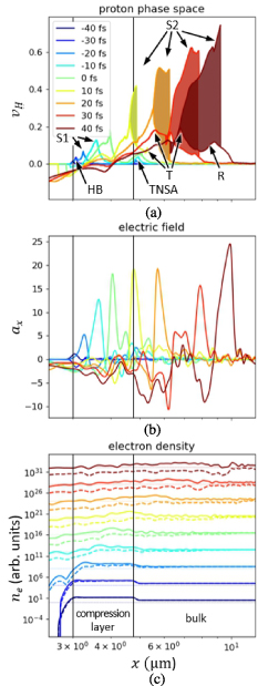
Figure 8. (a) Proton phase space, (b) accelerating electric field and (c) electron density  (solid) and relativistically corrected electron density
  (dashed) for various timesteps before and during RTF-RPA. The ions accelerated by RTF-RPA in the compression layer (S1) are trapped by RTF-RPA in the bulk and are further accelerated (S2). Ions initially at rest or accelerated by TNSA are not trapped and gain only little energy from the RTF passing them, (R), (T), respectively.
Download figure:
Standard image High-resolution image2.3.1. Lower laser intensity.
We now want to discuss an important benefit of the front compression layer specifically at smaller laser intensities,  , and short-pulse durations,
  , where RTF-RPA is less effective or even non-existent in homogeneous plasmas, cf figure 4. As a reason for this problem, we discuss that the matching between the RTF edge velocity and the ion acceleration cannot be established in these cases. To illustrate this, we show two cases with homogeneous density n0 close to each other (4 and 5 nc
) in figure 9 tor
, where RTF-RPA is less effective or even non-existent in homogeneous plasmas, cf figure 4. As a reason for this problem, we discuss that the matching between the RTF edge velocity and the ion acceleration cannot be established in these cases. To illustrate this, we show two cases with homogeneous density n0 close to each other (4 and 5 nc
) in figure 9 tor  and
and  . The problem can readily be seen in that for low density ((a), (d)), the laser propagates too fast, while for a slightly higher density ((c), (f)) the ions are reflected in hole boring like acceleration and the laser cannot keep up with them. Even as we tried densities closer to each other we could not find RTF-RPA in between, i.e., there appears to be a sudden jump from transparency regime to hole boring.
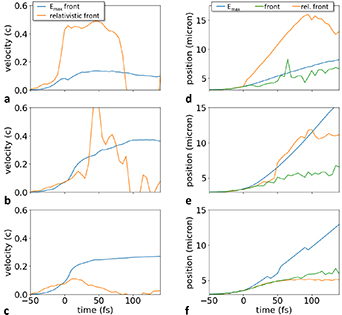
Figure 9. (a)–(c) Temporal evolution of the laser front velocity (orange) and velocity of the fastest ions (blue). (d)–(f) Temporal evolution of the respective positions of the point of laser reflection (orange) for two close initial plasma densities and homogeneous profile ( )
)  ((a), (d): transparent regime) and
  ((c), (f): hole boring regime) at
  ; and for the optimised RTF-RPA case with front compression,
  ,
,  , d = 1.6 (b), (e).
Download figure:
Standard image High-resolution imageIntroducing a finite pre-compression layer changes the situation drastically, see figure 10. We can now see the same qualitative behaviour as for high laser intensity. The pre-compression layer shifts the optimum density of the bulk to lower values. At the same time, the maximum ion energy increases with increasing thickness of the compression layer, reaching a maximum value of approximately twice that of the homogeneous plasma. At this optimum RTF-RPA is well established, as indicated by the close vicinity of the most energetic ions and the point of the laser reflection witnessed in figures 9(b), (e) and 11. The front compression layer keeps the laser slow at the beginning and gets faster after boring through, enabling the RTF-RPA process. Consequently, we can expect that for a pre-compressed target RTF-RPA can be effective even for low laser intensities, specifically in plasmas near the critical density and compression to modest density  .
.
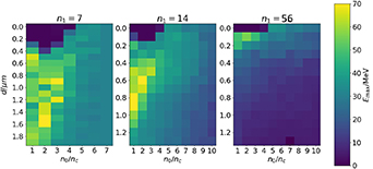
Figure 10. Maximum proton energy after the acceleration process with laser strength  ,
,  after laser peak arrival on target as a function of rear layer density n0 and front layer thickness d for front layer density
  (from left to right).
Download figure:
Standard image High-resolution image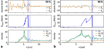
Figure 11. Plasma dynamics for the optimum front layer configuration at  :
:  ,
,  ,
,  .
.
Download figure:
Standard image High-resolution image2.3.2. 3D simulations.
It is important to note that the RTF-RPA process, and also the enhanced two-phase acceleration, can also be observed in 3D. This is to be expected since the RTF-RPA process is essentially a 1D process, but for future experimental realizations the applicability in 3D has to be checked and analyzed. We verified the effectiveness of the front compression layer by conducting exemplary 3D simulations for homogeneous and front compressed plasmas using PIConGPU [45]. The laser peak intensity and duration were kept as before in 1D, now with a tight focus of  FWHM. Figures 12 and 13 show the RTF edge and ion front velocities along with the profiles of electric fields, ion energies and plasma densities for the two optimal cases of a homogeneous and two-layered target, respectively. The ion energies are somewhat smaller in both cases than those observed in 1D geometry before, but again, we observe a substantial increase in the compression front plasma compared to the homogeneous plasma by more than
  .
.
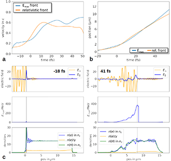
Figure 12. Lineouts along the laser axis showing the plasma dynamics for the 3D simulation. Target density is  , which is the optimal case for a homogeneous target and the chosen laser of
  and a transversal width of
  at FWHM.
Download figure:
Standard image High-resolution image
Figure 13. Lineouts along the laser axis showing the plasma dynamics for the 3D simulation with compressed front layer. An optimal configuration for the same laser parameters has a front layer density  ,
,  and a bulk density of
  .
.
Download figure:
Standard image High-resolution image
Thus, the qualitative behaviour of the system with varying parameters does not essentially differ, though some quantitative differences can be noted: the thickness of the compression layer that enhances the final energies is higher than for the 1D optimum, and also the density of the RTF-RPA optimum with a homogeneous target is higher than in the 1D case. The latter is due to an increased laser strength due to self-focusing in the target, and transversally pushing the density away from the laser axis.
3. Conclusions
Synchronized ion acceleration by slow light in a near critical plasma is an effective means of dramatically increasing ion cutoff energies in comparison to the classical TNSA approach. We have shown that the the maximum RTF-RPA ion energies can be obtained from a simple semi-analytic model and the EOM was constructed. This allows to predict the temporal evolution during RTF-RPA as well as the optimum combination between the laser parameters pulse duration, intensity, and the plasma density. We validated the model with a series of 1D PIC simulations, finding that the relationship between optimum density and pulse duration leads to maximum ion energy at the smallest density and highest possible pulse duration. For fixed laser pulse energy the shortest pulse duration is expected to yield the most energetic ions at the respective optimum plasma density, as long as RTF-RPA is still active. For longer pulse durations we see a significant reduction of the simulated optimal energies compared to the theoretical maxima due to dephasing of the process for long interaction times. This in practice limits the pulse durations yielding optimized RTF-RPA to values below about 100 fs for current state-of-the art laser systems.
Even higher ion cutoff energies can be reached with an optimized plasma density profile. We demonstrated this in a proof-of-principal type geometry of a two-layer plasma density profile. By increasing the density in the front of the target and decreasing the density of the bulk in the rear, the RTF is synchronized better to the accelerating protons, which can then keep up with the former longer. We verified the principal effect in 3D simulations and at low laser intensity where RTF-RPA is not effective in homogeneous density plasmas. These results could be extended in the future by more simulations to find the optimum combination of plasma density and pulse shape for realistic conditions. This, however, requires the optimization of many parameters, such as laser contrast, pulse duration, waist and dispersion, and plasma shape at the same time. Here, the extension of the model to include e.g. 3D effects and the plasma density shaping by the laser could be essential to accelerate such optimization.
Acknowledgments
This work was partially funded by the Center of Advanced Systems Understanding (CASUS), which is financed by Germany's Federal Ministry of Education and Research (BMBF) and by the Saxon Ministry for Science, Culture and Tourism (SMWKT) with tax funds on the basis of the budget approved by the Saxon State Parliament.
Data availability statement
The code SMILEI [39] used for the simulations was published under the CeCILL license and PIConGPU was published under GNU General Public License 3 [45].
The data that support the findings of this study are openly available at the following URL/DOI: 10.14278/rodare.1199.
Appendix
The mathematical derivation of the factor P which we introduced in b in equation (3) and which changes the penetration velocity for linear polarization can be seen as follows, following the steps outlined in [38]. The derivation starts with equation (2) in [38] which reads for linear polarization (in our dimensionless unit system)

where  . Hence the assumptions that lead to equations (3) and (4) in [38] are still valid. In the following we use equation (5) in [38] in a slightly modified form,

i.e. adding a factor  . In our simulations for linear polarization this modified expression shows good agreement with all our simulations: E.g. in figure 2(c) we can extract from the blue line in the lower panel (i.e.
  )
)  and with
  equation (12) gives
  , which compares reasonably well to
  in the simulation, cp. blue line for Ey
in figure 2(a) top panel. The difference of
in the simulation, cp. blue line for Ey
in figure 2(a) top panel. The difference of  compared to equation (5) in [38] is clearly due to incomplete evacuation of the electron density in the plasma wave, finite electron sheath thickness, and inhomogeneous background ion distribution.
In fact, also for circular polarization this modified expression seems to fit reasonably well, cp. simulation figure 1(a) in [38]  and the result of equation (12) for the respective parameters (
 ,
,  ,
,  ) gives
  .
.
We now follow the derivation of equation (8) in [38]. There,  was put into equation (7) to account for the relativistic mass increase in the plasma wave. In the simulation of figure 1 in [38], using circular polarization, the authors state in that empirically '
 is about half of
  '
'  . Our simulation for
  at linear polarization shows that the average of the reciprocal of γ,
  , i.e. about
  . These two expressions put into equation (7) in [38], together with the additional factor
  in equation (12), lead to equation (8) in [38] then reading for circular polarization

and for linear polarization:
Together with equation (4) we then recover equation (9) in [38] for circular polarization:
and obtain for linear polarization:
Hence,

This can be solved as outlined in [38] for βf
, yielding equation (3). It is in very good agreement with our 1D simulations both in terms of βf
as well as  and
and  .
.