

Abstract
Objective. Multi-parametric MR image synthesis is an effective approach for several clinical applications where specific modalities may be unavailable to reach a diagnosis. While technical and practical conditions limit the acquisition of new modalities for a patient, multimodal image synthesis combines multiple modalities to synthesize the desired modality. Approach. In this paper, we propose a new multi-parametric magnetic resonance imaging (MRI) synthesis model, which generates the target MRI modality from two other available modalities, in pathological MR images. We first adopt a contrastive learning approach that trains an encoder network to extract a suitable feature representation of the target space. Secondly, we build a synthesis network that generates the target image from a common feature space that approximately matches the contrastive learned space of the target modality. We incorporate a bidirectional feature learning strategy that learns a multimodal feature matching function, in two opposite directions, to transform the augmented multichannel input in the learned target space. Overall, our training synthesis loss is expressed as the combination of the reconstruction loss and a bidirectional triplet loss, using a pair of features. Main results. Compared to other state-of-the-art methods, the proposed model achieved an average improvement rate of 3.9% and 3.6% on the IXI and BraTS'18 datasets respectively. On the tumor BraTS'18 dataset, our model records the highest Dice score of 0.793(0.04) for preserving the synthesized tumor regions in the segmented images. Significance. Validation of the proposed model on two public datasets confirms the efficiency of the model to generate different MR contrasts, and preserve tumor areas in the synthesized images. In addition, the model is flexible to generate head and neck CT image from MR acquisitions. In future work, we plan to validate the model using interventional iMRI contrasts for MR-guided neurosurgery applications, and also for radiotherapy applications. Clinical measurements will be collected during surgery to evaluate the model's performance.
Export citation and abstract BibTeX RIS

Original content from this work may be used under the terms of the Creative Commons Attribution 4.0 licence. Any further distribution of this work must maintain attribution to the author(s) and the title of the work, journal citation and DOI.
1. Introduction
Magnetic resonance imaging (MRI) is a noninvasive imaging technique used for several clinical applications such as lesion classification schemes, hemorrhage detection, and segmentation for tumor burden assessment (Chartsias et al 2017, Zhou et al 2020, Liu et al 2021, Peng et al 2021, Touati et al 2021). Multi-parametric MRI is frequently used to characterize soft-tissue pathologies, as it can capture a wide diversity of contrasts in soft tissues of the same anatomy (Raju et al 2020). Hence, for the same subject, a specific MRI pulse sequence can generate different contrast characteristics in soft tissues, i.e. each contrast representing a particular image appearance (Raju et al 2020). Amongst the most common MRI sequences in tumor analysis, the T1-weighted MRI (T1-MRI) scans are more appropriate for the delineation between gray and white matter in brain images, while T2-weighted MR (T2) images allows to improve the distinction between fluid and cortical tissue (Dar et al 2019, Touati et al 2021). The fluid attenuated inversion recovery (FLAIR) sequence can be used to suppress the cerebrospinal fluid effects. The T1-weighted contrast-enhanced (T1ce) images are mostly used to enhance tumor regions in brain images. The magnetic resonance angiography (MRA) is predominantly used to evaluate vascular anatomy diseases such as the detection of vessel abnormalities which can lead to hemorrhages (Olut et al 2018). Finally, the proton density image (PD) is extensively applied in radiology (Arnold et al 1994, Beaulieu et al 1998, Tofts 2003) and can be used to infer water content (Tofts 2003) for lesion classification schemes or multispectral segmentation (Tofts 2003). These multimodal MRI scans provide complementary information that increases sensitivity for tumor heterogeneity, instead of considering only a single imaging contrast. However, different technical and practical conditions may limit the acquisition of various MR imaging modalities such as additional cost of scanning time, limited scanner availability for acquiring multiple sequences, or missing some modalities due to imaging/motion artifacts and safety precautions (Dar et al 2019, Yu et al 2019). These particular conditions in clinical practice are often inevitable and affect mostly the diagnosis or treatment quality. To address these limitations, image reconstruction approaches can be adopted to generate the unavailable scan required for radiotherapy treatment planning. Multimodal image synthesis is an efficient synthesis solution that automatically generates missing MRI sequences from the different available modalities (Chartsias et al 2017, Zhou et al 2020). This challenging task avoids the acquisition of actual scans and provides the unavailable MRI modality necessary for diagnosis and treatment.
Amongst works proposed for the multimodal MRI synthesis problem, we can include the cycle constrained adversarial model, which is based on conditioned autoencoders and multitask learning (Liu et al 2021). The diffusion learning model of Özbey et al (2022) relies on an unsupervised conditional adversarial diffusion framework, which is trained using a cycle-consistent architecture on unpaired data. The model relies on two generator/discriminator pairs and comprises a non-diffusive module that generate initial paired source images, which are then used used in the diffusive module s prior to generates the target contrast. The model in Dar et al (2022) also proposed an adversarial learning framework, but based on adaptive diffusion prior for MRI reconstruction. The framework employ two reconstruction phases, a rapid-diffusion phase to estimate an initial reconstruction using the trained diffusion prior, and an adaptation phase to refine the result by updating the prior to minimize the reconstruction loss on acquired data. Finally, the introduced model in Dalmaz et al (2022) proposes a synthesis approach based on a conditional adversarial learning using a vision transformer generator. The framework consists of a convolutional and transformer streams that rely on a residual bottleneck. The bottleneck comprises an aggregated residual transformer block. The model of Korkmaz et al (2022) proposes a zero-shot framework based on long-range dependency of transformers for unsupervised MR reconstruction. It consists of prior-learning and zero shot inference stages. The transformer based generative model is trained to minimize the error between the network output and the fully-sampled multi-coil MR acquisitions. The proposed model in Yu et al (2019) introduces an edge-aware generative adversarial network. The proposed framework includes a generator, a discriminator, and a Sobel edge detector, to better capture the high frequency details in the target image. This framework incorporates edge information in the generator and the edge similarity is adversarially learned via the discriminator. The synthesis model of Peng et al (2021) includes a confidence-guided aggregation module for fusing modality specific features and a cross-modal refinement module to refine the generated target image. The model is trained in an end-to-end generative adversarial manner using two generators supervised by one discriminator. The introduced adversarial model in Zhan et al (2021) relies on a gate merging mechanism for multimodal features fusion, and uses a combination of adversarial, pixel-wise loss and gradient differential losses for the network training. The multi-level transfer generative approach (Yurt et al 2021) relies on a mixture of one-to-one and many-to-one streams to extract multi-level features, which are then concatenated in an adversarial fashion. We can also include the multi-modality MRI synthesis model (Xin et al 2020) which makes use of three generator networks via the Pix2Pix architecture (Zhu et al 2017), or the hybrid-fusion network (Hi-Net) (Zhou et al 2020) that utilizes a modality-specific network to extract features from each modality, and then uses a densely fusing network to fuse the multimodal hierarchical features into one common space. Many other multimodal MRI synthesis approaches try to build a common feature space from different imaging modalities (Chartsias et al 2017, Yang et al 2019), using GAN architectures with supervised (Chartsias et al 2017) or semi-supervised learning techniques (Yang et al 2019). The extended GAN synthesis model (Olut et al 2018) incorporates the Huber loss (Friedman et al 2001) and a set of steerable filters for MRA image generation. The model proposed in Joyce et al (2017) is composed of one encoder for each corresponding imaging modality to embed the different images into different representations. The obtained representations are aligned using a spatial transformer module (Jaderberg et al 2015) and then fused in a shared latent representation from which a decoder generates the target contrast. While these approaches can effectively generate high-resolution synthetic images (Chartsias et al 2017, Xin et al 2020, Zhou et al 2020, Liu et al 2021), multimodal MR synthesis task is still a challenging problem. One of the main challenging problem is to reconstruct high resolution images in pathological MR images, for improving clinical analysis and diagnosis. Particularly, in tumor cases that appear in a wide variety and complex shapes (Egeblad et al 2010). Also, generating MR images that avoids oversmoothing, missing details or blurred remains an unsolved problem (Liu et al 2020). In such cases, local artificial pathology may occur in the generated sMR contrasts affecting the existing pathology structure.
Contrary to state-of-the-art multimodal synthesis approaches, we propose a multimodal MRI synthesis approach based on paired feature representations. Our approach is based on a contrastive learning framework and aims to train a bidirectional model to synthesize the target MRI from a common feature space that approximately matches the target feature space. First, we extract a relevant feature representation from the images of the target modality. We adopt an unsupervised contrastive learning strategy to train an encoder to extract a pair of features from the target space. To learn such a representation from the target feature space (the target modality), each input image is first transformed into a pair of augmented representations containing different information on the same patient. Then we train a contrastive loss on the augmented pairs. Second, we train a synthesis network using a bidirectional multimodal synthesis loss based on contrastive feature pairs. We incorporate a bidirectional synthesis loss that learns the best matching between the encoding features of the input and the learned target features so that we can optimally transform from one feature space to another. This process is done in two opposite directions using a triplet loss (Schroff et al 2015) defined in the embedding space. Moreover, the architecture of the model does not learn to synthesize the target modality from the original multi-channel (2) input images, but rather from its augmented representation, which is based on a pair of complementary features. This pair of features encodes both image intensity and structural information for each input modality.
2. Proposed bidirectional MRI-synthesis model
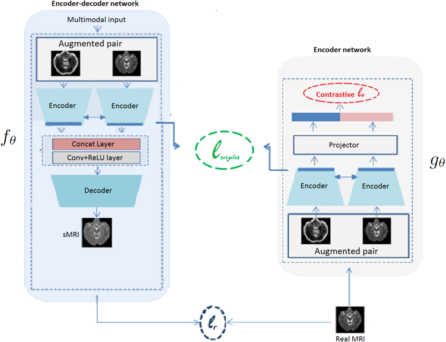
In our application, we make use of an encoder gθ that projects the augmented pair of the target images into different vector representations for target feature learning. We adopt an encoder–decoder network fθ that synthesizes the target image modality from the other augmented multimodal image inputs. The goal is to find a common feature space from two heterogeneous feature representations, that subsequently improves the decoding learning process to generate the target modality from various imaging modalities (see figure 1).
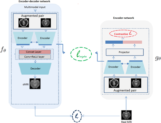
Figure 1. Overall scheme of the multi-parametric MRI synthesis architecture based on a paired learning architecture with two different networks fθ and gθ . The encoder network gθ consists of an augmented pairwise module, one Siamese network with a shared weight between the two encoder CNN streams, and one hidden layer for the projector. The encoder–decoder network fθ relies on a multi-channel U-net architecture and consists of one encoder Siamese network based on an augmented pair, concatenation and convolutional layers, and one decoder block. While the weights of the reconstruction network fθ are frozen, we train the encoder gθ using the contrastive loss ℓ c . We train the encoder–decoder fθ with gθ frozen by minimizing the overall cost function given in equation (3).
Download figure:
Standard image High-resolution image2.1. Feature representation learning
In this stage, we build the target feature space using an efficient unsupervised learning contrastive approach (Wu et al 2018, Chen et al 2020, He et al 2020). We train an encoder gθ via a pairwise contrastive loss (Chen et al 2020) on the augmented pairs of the target space. The augmented pair includes two image representations of the same input. At each training step, we select randomly a batch of N images. For these N images in a batch, we first capture the intensity information of the N images (Chen et al 2020). Second, we compute the image gradient magnitude using the data augmentation operator based on high-frequency filter (Chen et al 2020).
2.1.1. Pairwise contrastive loss
Given one image input, the positive pair is the augmented pair belonging to the same image input, while the negative pair is the augmented pair belonging to an unrelated image. We compute the contrastive loss ℓ c (Chen et al 2020) on the augmented MRI pair. For all positive pairs in the augmented batch, the overall contrastive loss ℓ c is defined by equation (1). For each positive pair of the same image, the contrastive loss ℓ ij is calculated by equation (2) (Chen et al 2020):


where zi and zj are the encoded vectors, zk are the other projected vectors of the other images in the batch, τ is a positive scalar temperature parameter, 1 is an indicator function that returns 1 if k ≠ i else 0, N is the batch size which is augmented to 2N images, and zi · zj is the dot product similarity measure between the vectors.
2.2. Network architecture
2.2.1. Encoder gθ
The encoder gθ includes two components. The first component extracts the embedding representation of the augmented pair images. We use a pairwise learning architecture that relies on the Siamese network and consists of two parallel CNN streams with shared weights. The second component is a projection network that converts the resulting paired representation into suitable low-dimensional feature vectors for contrastive loss calculation. We adopt a multi-layer perceptron (Hastie et al 2009) composed of one hidden layer as a projection network. For the feature image extraction, the Siamese network has five (5) layers and progressively down-sample the input through four 4 scales. In the first four layers, each CNN stream makes use of two convolutional layers followed by an activation function (ReLU), and one max-pooling operation. In the last layer, we use two convolutional operations with an activation function ReLU. We applied a convolutional filter size of 3 × 3. We used a stride of 2.
2.2.2. Encoder–decoder network fθ
For the multimodal synthesis problem, the different modalities are obtained from the same patient and are co-registered to each other, for different subject acquisitions. To this end, we rely on a multi-channel architecture which is well adapted for paired data to infer relevant multimodal image features, and thus, the correlation through the different images (Lavdas et al 2017). Therefore, we concatenate the different input modalities as different input channels xi . We adopt a multi-channel U-net (Ronneberger et al 2015) learning architecture that outputs a single image modality in the last layer. It is based on an augmented pair with complementary information and consists of an encoder and decoder networks. We feed the multi-channel augmented input to the encoder part, where we transform the paired multi-channel images through different scales, using Siamese architecture, which makes use of the VGG16 model for each branch. The encoded features resulting in the latent space are then concatenated via the concatenation layer and then fed to the convolutional and ReLU layers. For the decoding stage, the decoder part ensures to output the target modality from the encoding feature representation. We repeat the same process as the encoding step, but we apply a set of 2 × 2 up-sampling transpose convolutional operations, two 3 × 3 convolutional operations with an activation function ReLU, until achieved the last layer that outputs the synthesized MRI image.
2.3. Multimodal image synthesis loss
In the proposed model, we use the original target space and its contrastive learned features for training the encoder–decoder network fθ based on augmented input image modalities (n = 2). We reformulate our bidirectional synthesis loss as the combination of the ℓr and ℓtriplet terms In order to train the synthesis network fθ , we optimize the overall loss ℓ expressed in equation (3)

where ℓ r is the reconstruction loss. The ℓtriplet term is the bidirectional multimodal matching loss based on triplet of feature pairs, and λ1 is the weight for the ℓtriplet term.
We compute the differences between the real and generated MR sequences via the ℓr term. We impose on the ℓ r loss, the complementary regularization ℓtriplet defined in equation (5), for learning a multimodal feature matching, in two opposite directions, between the embedding space of the target modality gθ and all input modalities fθ . In other words, our approach learns to match the latent representation between the input modalities and output modality, ensuring that it contains relevant features across multiple modalities and similar to the desired target modality.
The reconstruction loss ℓ r is given in equation (4) and is expressed by the L2 norm (Snell et al 2017):

where  is the sMRI for the ith MRI training observation, mi
is the corresponding target modality, and
is the sMRI for the ith MRI training observation, mi
is the corresponding target modality, and  is the augmented multi-channel input representing the different imaging modalities through a pair of images 〈s, t〉.
2.4. Bidirectional multimodal feature matching
We seek to learn a common feature space, which is more similar to the target feature image space, i.e. training the network fθ
to transform the input in the same feature representation of the target image, from which the target contrast is synthesized. This allows us to embed the augmented multi-channel input  in an encoding feature space that corresponds approximately to the target encoding space, so that the network fθ
synthesizes the target contrast from an embedding feature space that characterizes the target images thanks to the target learned features. To address this problem, we rely on feature matching based on augmented pairs, to learn an embedding space that has the best matching with the target feature space. We learn to find a matching between the latent feature space resulting from the encoder part of the network fθ
and the learned target space resulting from the encoder gθ
.
in an encoding feature space that corresponds approximately to the target encoding space, so that the network fθ
synthesizes the target contrast from an embedding feature space that characterizes the target images thanks to the target learned features. To address this problem, we rely on feature matching based on augmented pairs, to learn an embedding space that has the best matching with the target feature space. We learn to find a matching between the latent feature space resulting from the encoder part of the network fθ
and the learned target space resulting from the encoder gθ
.
2.4.1. Multimodal feature matching
One way to build the common space is to learn a single matching function between the two encoded feature spaces, using either a metric learning approach or employing directly the L2 distance for matching the two spaces based on the computed similarity. Nevertheless, these matching strategies remain less suited for matching two latent spaces that are extracted from two heterogeneous representations through different encoder networks. In such a case, this learning strategy based on single matching is less effective to reduce the mismatched learned feature pairs, which decreases the learning performance and consequently affects the generalization ability of the model. Therefore, incorporating an efficient matching learning strategy in the network fθ
is necessary, so that it reduces the learned mismatched feature pairs and better captures the variation between the two spaces, so that transforms between the multi-channel input to the real target output feature space are optimal. Given a pair of input/output encoding feature space  and gθ
(. ), there are two different solutions to the matching problem, where the feature space
and gθ
(. ), there are two different solutions to the matching problem, where the feature space  should match the one of gθ
(. ). In the first direction, we use features from
should match the one of gθ
(. ). In the first direction, we use features from  to find its corresponding features in the space gθ
(. ). In the second direction, we inversely use features from gθ
(. ) to find the matches in the
to find its corresponding features in the space gθ
(. ). In the second direction, we inversely use features from gθ
(. ) to find the matches in the  space. To further reduce the mismatched pairs, we rely on a pair of image representations 〈s, t〉, that helps to preserve the mapping for both image intensity and structural information in the embedding space. Thus, we consider a double-feature-matching learning strategy based on augmented pairs, that does not only match the pairs of features
  ∈
∈ ,
,  ∈ gθ
(. ) in one direction or the other, but also takes into account both existing directions for matching the feature pairs, hence a bidirectional solution. We thus force the network fθ
to reduce not only the mismatched pairs considered in the learning process, but also to generate a synthetic MRI image from common features that are learned in two complementary and opposite directions. To achieve this goal, we design an efficient double-feature-matching strategy, that relies on all possible pairs of convolutional maps, existing between the transformed feature pair
∈ gθ
(. ) in one direction or the other, but also takes into account both existing directions for matching the feature pairs, hence a bidirectional solution. We thus force the network fθ
to reduce not only the mismatched pairs considered in the learning process, but also to generate a synthetic MRI image from common features that are learned in two complementary and opposite directions. To achieve this goal, we design an efficient double-feature-matching strategy, that relies on all possible pairs of convolutional maps, existing between the transformed feature pair  and
and  . We model our double-feature matching strategy using a bidirectional triplet loss based on pairs. This allows us to better measure the difference between the two heterogeneous spaces
  and gθ
(. ), that exhibit radically different nonlinear scale factors, i.e. different image feature statistics.
and gθ
(. ), that exhibit radically different nonlinear scale factors, i.e. different image feature statistics.
2.4.2. Bidirectional triplet loss
The primary objective of the bidirectional triplet loss is to learn a matching function. Instead of considering a single corresponding feature f〈s,t〉, the matching function uses a pair of corresponding features (f〈s,t〉,  ) belonging to the same space. Each feature representation f〈s,t〉 is a pair of features extracted from the augmented pair 〈s, t〉. The goal is to learn a matching loss that encourages to assign a smaller distance to the best matched pairs than between mismatched pairs. To satisfy this, we rely on a metric learning method that match the two spaces by comparing features (Schroff et al
2015). We adopt a triplet loss (Schroff et al
2015) as a matching measure (Wang et al
2019), using a pairwise distance that measures the similarity between two different feature pairs, thus enforcing to build a function which captures the relationship between a pair of representations (each representation is a pair) (Schroff et al
2015). Furthermore, in this particular scenario, we aim to learn the mapping for a bidirectional feature matching. Precisely, we seek to minimize a bidirectional triplet loss, where our double-feature matching learning strategy should be verified in both directions. In addition, the bidirectional matching loss seeks to learn the best matching through a pair of features extracted from the augmented pair 〈s, t〉.
) belonging to the same space. Each feature representation f〈s,t〉 is a pair of features extracted from the augmented pair 〈s, t〉. The goal is to learn a matching loss that encourages to assign a smaller distance to the best matched pairs than between mismatched pairs. To satisfy this, we rely on a metric learning method that match the two spaces by comparing features (Schroff et al
2015). We adopt a triplet loss (Schroff et al
2015) as a matching measure (Wang et al
2019), using a pairwise distance that measures the similarity between two different feature pairs, thus enforcing to build a function which captures the relationship between a pair of representations (each representation is a pair) (Schroff et al
2015). Furthermore, in this particular scenario, we aim to learn the mapping for a bidirectional feature matching. Precisely, we seek to minimize a bidirectional triplet loss, where our double-feature matching learning strategy should be verified in both directions. In addition, the bidirectional matching loss seeks to learn the best matching through a pair of features extracted from the augmented pair 〈s, t〉.
If we assume a triplet of features pairs  , we denote
  as a positive pair, which includes two features, one anchor feature fa
and one positive feature fp
that belong to the same space fθ
(. ). The feature
as a positive pair, which includes two features, one anchor feature fa
and one positive feature fp
that belong to the same space fθ
(. ). The feature  is a negative feature belonging to the space gθ
(. ). Analogously for the opposite direction. We recall that each feature is a pair of features extracted from the augmented pair 〈s, t〉. Then, we reformulate in equation (5) the bidirectional matching loss based on a triplet of feature pairs, for learning a double-feature matching. The equation (5) is an unsupervised contrastive learning metric that aims to learn the difference between the data of interest and some reference data. In our case, it captures inherent features and representations for MR images
is a negative feature belonging to the space gθ
(. ). Analogously for the opposite direction. We recall that each feature is a pair of features extracted from the augmented pair 〈s, t〉. Then, we reformulate in equation (5) the bidirectional matching loss based on a triplet of feature pairs, for learning a double-feature matching. The equation (5) is an unsupervised contrastive learning metric that aims to learn the difference between the data of interest and some reference data. In our case, it captures inherent features and representations for MR images

where D(. ) is the similarity measure function computed by the  norm in the embedding space. Here,
  and
and  are the two opposite feature anchors sampled in bidirectional manner from the fθ
(. ) and gθ
(. ) spaces, with α as the margin. Lastly,
are the two opposite feature anchors sampled in bidirectional manner from the fθ
(. ) and gθ
(. ) spaces, with α as the margin. Lastly,  is the hard positive and
  is the hard negative. In our application, the positive and negative samples are selected using a hard sample selection strategy (Schroff et al
2015). Moreover, in our case, we adopt a hard selection strategy which selects the hard sample via a pair of features. The hard positive
is the hard negative. In our application, the positive and negative samples are selected using a hard sample selection strategy (Schroff et al
2015). Moreover, in our case, we adopt a hard selection strategy which selects the hard sample via a pair of features. The hard positive  is obtained using equation (6), and the hard negative is selected using the equation (7). Analogously for the second direction. The total loss is the summation of all possible pairs in the two feature spaces


Here, the hard positive  represents the largest neighbor to the anchor fa
in terms of
represents the largest neighbor to the anchor fa
in terms of  distance, using a pair of features. Inversely, the hard negative
  represents the nearest neighbor to the anchor fa
.
represents the nearest neighbor to the anchor fa
.
2.5. Network parameter settings and architecture details
For the experiments, the proposed model was trained with the Adam optimizer (Kingma and Ba 2015) using the optimal parameters for the margin α and temperature τ, that were obtained on the brain BraTS'18 data (see section 3.2). We fixed the margin α to 0.2, and the dimension number to 4096 with a scalar temperature τ of 0.05. The learning rate was set to 0.001, and the maximum number of epochs to 300. We used a momentum value of 0.5. We set the weight λ1 to 1. The batch size was set to 32. For the encoding phase, the convolutional feature maps number was respectively set to {32, 64, 128, 256, 512} for both networks fθ and gθ . The decoding feature maps number was set to {256, 128, 64, 32, 1} for the network fθ . The contrastive component gθ takes an augmented shape input (64, 256, 256) (i.e. there are 32 pairs of images), which is processed through the Siamese encoder to extract 512 feature maps of shape (64, 16, 16, 512). These are then reduced via the projector to (64, 4096) encoded vectors, which are then sent to determine the contrastive term ℓ c . We used the trained encoder gθ in the second stage, for training the reconstruction network fθ . At this level, we discarded the projector from the trained encoder gθ , and we only kept its Siamese encoder that extracts a pair of (512, 16, 16) features from the ith augmented observation of the target space. The encoder–decoder fθ takes a multi-channel input (two modalities in our case) of size (256, 256, 2) and augmented it to (256, 256, 4), then encoded these augmented inputs through its Siamese block to extract a pair of (16, 16, 512) features. The two feature representations were then concatenated (16, 16, 1024) and reduced to an encoded representation of shape (16, 16, 512) in the middle layers. This reduced representation was finally fed to the decoder block to synthesize an output of (256, 256, 1) of the desired modality. We trained the encoder–decoder fθ with gθ frozen, by minimizing the overall cost function ℓ. Otherwise said, we train the two networks separately.
3. Experimental results
3.1. Dataset descriptions
For the experiments, we consider two different multimodal brain datasets: the multimodal brain tumor segmentation BraTS'18 (Menze et al 2014) and the IXI brain datasets (Sohail et al 2019).
3.2. Experimental settings
The BraTS'18 dataset was randomly divided into 80% training set and 20% test set. We conducted an experiment using a basic model based on single feature matching for tuning the parameters of the contrastive model. To find the optimal parameters of the proposed synthesis model, we chose the best configuration that outputs the lowest mean absolute error (MAE) on the testing data (20%), for generating the T2 from pairs of T1ce and FLAIR multi-channel input. We performed a grid search in a defined parameter space, which includes the margin α, the scalar temperature τ, and the dimension number parameters. This parameter space allows tuning the margin α for optimizing the feature embedding (Zhang et al 2019), and the temperature parameter τ to improve the separation between the positive and negative pairs (Wang and Liu 2021). We used a grid search optimization technique that explored different parameter settings. The two parameter values α and τ, respectively, varied in the range (0.05, 0.4) and (0.005, 0.5), using a fixed factor of 2 and 10. The dimension number varied in the range of (2048, 8192) using a factor of 2. The training/validation process was repeated for each configuration in the parameter space. The optimal MAE was 77 ± 3.63 and is obtained using a margin α of 0.2 and a temperature τ of 0.05 with a dimension number of 4096.
3.3. Ablation study
We validated the synthesis model on the public multimodal brain IXI scans, using the optimized values learned on the BraTS'18 data. We compared the synthesis performance of the proposed model with and without feature matching based on contrastive learning component, under the same testing conditions. We also compared the synthesized results yielding by the proposed model using a single and a double feature matching learning strategies. We experimented the model to synthesize one brain imaging modality from two other modalities, using all possible combinations between T2, PD, and MRA brain images. We used the Kolmogorov–Smirnov test to test data normality. The statistical test recorded was 0.11 with a p-value of 0.44. Figures 2–4 show qualitative comparison results. For model evaluation, we computed the MAE, structural similarity index measure (SSIM), and peak signal-to-noise ratio (PSNR) measures (Dong et al 2017) (see tables 1–3). We also evaluated the model performance in terms of histogram distribution shape using the Bhattacharyya score (BC) (Kailath 1967) (see table 4 and figure 5). Finally, we evaluated the model performance using a statistical test based on testing hypothesis. We used the two sample Z-tests under the null hypothesis with a desired confidence of 5% (Gravetter et al 2020) (see table 5).

Figure 2. Synthesis sT2 comparison results for different sample patient scans, using multichannel input MRA and PD.
Download figure:
Standard image High-resolution image
Figure 3. Synthesis sPD comparison results for different sample patient scans, using multichannel input MRA and T2.
Download figure:
Standard image High-resolution image
Figure 4. Synthesis sMRA comparison results for different sample patient scans, using multichannel input T2 and PD.
Download figure:
Standard image High-resolution image
Figure 5. Comparative intensity histograms of the brain synthesized contrasts: T2, PD and MRA. (a): histogram of the target image. (b), (c): Obtained distribution histograms of the generated modalities by our multi-parametric model based on bidirectional and single feature matching learning strategies.
Download figure:
Standard image High-resolution imageTable 1. T2 synthesis results comparison. The synthesis results between our model based on bidirectional and single feature matching learning, and between the model without contrastive learning and based on single matching.
| Model | MAE ± STD | PSNR ± STD | SSIM ± STD |
|---|---|---|---|
| Without contrastive | 339 ± 6.03 | 15.15 ± 2.89 | 0.695 ± 0.01 |
| Single matching | 123 ± 4.17 | 25.42 ± 2.43 | 0.871 ± 0.04 |
| Double matching | 81 ± 3.56 | 31.45 ± 1.90 | 0.951 ± 0.06 |
Table 2. PD synthesis results comparison. The synthesis results between our model based on bidirectional and single feature matching learning, and between the model without contrastive learning and based on single matching.
| Model | MAE ± STD | PSNR ± STD | SSIM ± STD |
|---|---|---|---|
| Without contrastive | 357 ± 7.15 | 15.17 ± 2.05 | 0.676 ± 0.03 |
| Single matching | 113 ± 5.22 | 24.63 ± 1.50 | 0.887 ± 0.07 |
| Double matching | 59 ± 6.39 | 28.66 ± 1.30 | 0.926 ± 0.03 |
Table 3. MRA synthesis results comparison. The synthesis results between our model based on bidirectional and single feature matching learning, and between the model without contrastive learning and based on single matching.
| Model | MAE ± STD | PSNR ± STD | SSIM ± STD |
|---|---|---|---|
| Without contrastive | 248 ± 4.55 | 17.07 ± 2.57 | 0.713 ± 0.04 |
| Single matching | 93 ± 5.88 | 26.33 ± 1.93 | 0.921 ± 0.04 |
| Double matching | 74 ± 4.12 | 29.30 ± 1.75 | 0.945 ± 0.03 |
Table 4. Comparison of synthesis results in terms of histogram quality.
| Mappings | Model | BC ± STD |
|---|---|---|
| PD, MRA → T2 | Double matching | 0.899 ± 0.07 |
| Single matching | 0.854 ± 0.05 | |
| Without contrastive | 0.643 ± 0.02 | |
| MRA, T2 → PD | Double matching | 0.882 ± 0.06 |
| Single matching | 0.831 ± 0.04 | |
| Without contrastive | 0.612 ± 0.05 | |
| Double matching | 0.861 ± 0.08 | |
| PD, T2 → MRA | Single matching | 0.803 ± 0.05 |
| Without contrastive | 0.658 ± 0.04 | |
Table 5. Comparison of synthesis results based on testing hypothesis (statistical test). The test statistic used is the two sample Z-tests under the null hypothesis with a desired confidence of 5% i.e. at p < 0.05.
| Mappings | Model | Paired Z-test | P-value | Null hypothesis | Statistical difference conclusion |
|---|---|---|---|---|---|
| (PD, MRA) → T2 | Double matching | 1.3119 | 0.189 554 | Accept | Not significant |
| Single matching | 2.7728 | 0.005 558 | Reject | Significant | |
| Without contrastive | 4.6673 | 0.000 00 | Reject | Significant | |
| (T2, MRA) → PD | Double matching | 1.5671 | 0.117 091 | Accept | Not significant |
| Single matching | 2.6115 | 0.009 015 | Reject | Significant | |
| Without contrastive | 5.4298 | 0.000 00 | Reject | Significant | |
| Double matching | 1.4790 | 0.139 14 | Accept | Not significant | |
| (T2, PD) → MRA | Single matching | 2.0920 | 0.036 439 | Reject | Significant |
| Without contrastive | 8.8740 | 0.000 00 | Reject | Significant | |
3.4. Comparative methods
We compared our proposed model to three other state-of-the-art synthesis methods (Chartsias et al 2017, Zhu et al 2017, Zhou et al 2020). The first multimodal MR synthesis approach is the Hi-Net framework (Zhou et al 2020), which consists of three networks: a modality-specific network that learns to extract features from each modality, a multimodal fusion network that learns a common latent representation among input modalities, and finally a multimodal synthesis network that consists of a generator and a discriminator. The generator combines the latent representation with the extracted features to generate the target MR image. The discriminator discriminates between the generated and real images. The second multimodal MR synthesis method is the end-to-end MM-syns model (Chartsias et al 2017), which aims to transform the input modalities into a common invariant latent space to synthesize the target MR image from a single fused representation. The model utilizes one encoder for each input modality, a pixel-wise max function (Chartsias et al 2017) for feature fusion and a decoder network. Finally, the third method is a multi-channel conditional GAN that is based on a multi-channel U-net generator and a 32 × 32 PatchGan discriminator with a conditional GAN loss (Isola et al 2017). These methods were compared on BraTS'18 to synthesize the T2 from T1ce and Flair brain images, as well as all possible combinations between them. We also compared these methods on the IXI dataset in a similar fashion.
To further evaluate and compare the quality of the synthesized images against state-of-the-art methods, we compared the model performance for preserving tumor regions in the synthesized brain images. We compared the models under a tumor segmentation task performed on the synthesized images (Xin et al 2020, Liu et al 2021). We used a U-net (Ronneberger et al 2015) as a segmentation method to extract the tumor areas from the sT2 images. We trained the U-net segmentor on the tumor BraTS'18 dataset using the original T2 images, and then the built segmentation model was used to predict the tumor segmentation from the sT2 images.
3.5. Results
For all experiments, the reported results are the synthesis results of a single contrast generated from two multi-parametric source images. We report in tables 1–3 the obtained results for the ablation study. When training the model without contrastive learning, results presented in tables 1–4 show that the synthesis results are encouraging for all three contrasts. However, the model improves in performance when the feature matching based on contrastive component is included in the model. As an example, for generating the sT2, the model yields the best MAE of 81 ± 3.56, using the bidirectional feature matching based on the contrastive learning strategy. Without employing the feature matching based on the contrastive learning module, the model yields an MAE of 339 ± 6.03. Using only the L2 reconstruction loss for training the model, the matching between the features of the source and target contrast is ignored and in this case the model learns to minimize only the difference between the intensities of the generated and the target contrast.
For the synthesis results obtained by the proposed model based on the feature matching contrastive module, tables 1–4 show that employing a single feature matching strategy yields an improved synthesis results for synthesizing the three modalities. Meanwhile, training the model using the bidirectional feature matching strategy allows to achieve the best synthesis results in all three cases. While the model achieves a contrast enhancement SSIM score of 0.951 ± 0.06 or generating sT2, the model based on single matching achieves an SSIM score of 0.871 ± 0.04. In the sPD and sMRA tasks, the proposed model based on bidirectional feature matching achieves the highest BC scores of 0.882 ± 0.06 and 0.861 ± 0.08 for synthesizing the sPD and sMRA images, respectively. On the other hand, the model based on single feature matching reports the lowest BC scores of 0.831 ± 0.04 and 0.803 ± 0.05 for synthesizing both modalities. For the histogram intensity distributions obtained by the model based on double matching, the histograms intersect fairly with the histogram distribution of their ground truths compared to those obtained via the model based on single matching (figure 5).
Overall, when generating the sT2, sPD and sMRA, the improvement of the synthesis model based on a single matching module over the model without the contrastive component is {10.8%, 12.2%, 19.3%}. The performance of the model based on double feature matching improves by {2.1%, 2.7%, 2.3%} to the proposed model based on single matching for generating the three cases. From testing hypothesis table 5, the test statistic based on the paired Z-test under the null hypothesis at p < 0.05 shows that the statistical difference was not significant between the generated and the real images for the synthesis results obtained only by the described model based on double feature matching learning. As observed from table 6, the proposed model outperforms the state-of-the-art methods for synthesizing different contrasts, where the average improvement rate increases by 3.6% on BraTS'18 brain scans, and by 3.9% on IXI data compared to the best method (see table 7). Table 8 reports the tumor segmentation comparison results obtained on the sT2 image, where it achieves the best Dice score of 0.793(0.04). The proposed method achieved improved synthesis results with superior segmentation adaptation compared to other multimodal MR synthesis methods. Compared to the other methods, the proposed model directly captures a correlation of the image distribution. In contrast, the other GAN methods employ a common sampling process, which can limit sample fidelity and diversity of MR synthesized images.
Table 6. Comparison with state-of-the-art synthesis methods. The MR synthesis results are compared with two multimodal MR synthesis methods (Chartsias et al 2017, Zhou et al 2020) and one other generation method (Isola et al 2017). The MR results are obtained from two heterogeneous inputs: (T1ce, flair) → T2, (T2, flair) → T1ce, and (T2, T1ce) → flair (tumor BraTS'18 dataset), (PD, MRA) → T2, (T2, MRA) → PD, and (T2, PD) → MRA (IXI dataset).
| Mappings | Model | MAE ± std | PSNR ± std | SSIM ± std |
|---|---|---|---|---|
| BraTS'18 dataset | ||||
| (T1ce, flair) → T2 | Multichannel conditional GAN (Isola et al 2017) | 185 ± 4.81 | 20.88 ± 2.29 | 0.743 ± 0.01 |
| MM-Syns (Chartsias et al 2017) | 141 ± 3.54 | 22.12 ± 2.39 | 0.826 ± 0.05 | |
| Hi-Net (Zhou et al 2020) | 134 ± 3.17 | 23.75 ± 2.55 | 0.837 ± 0.04 | |
| Proposed model | 47 ± 4.14 | 29.52 ± 2.08 | 0.928 ± 0.07 | |
| (T2, flair) → T1ce | Multichannel conditional GAN (Isola et al 2017) | 191 ± 5.26 | 19.25 ± 1.96 | 0.767 ± 0.09 |
| MM-Syns (Chartsias et al 2017) | 138 ± 4.18 | 25.42 ± 1.38 | 0.849 ± 0.03 | |
| Hi-Net (Zhou et al 2020) | 129 ± 3.78 | 25.96 ± 1.42 | 0.854 ± 0.01 | |
| Proposed model | 62 ± 4.03 | 32.21 ± 1.72 | 0.916 ± 0.03 | |
| Multichannel conditional GAN (Isola et al 2017) | 171 ± 4.56 | 21.28 ± 1.69 | 0.814 ± 0.05 | |
| (T2, T1ce) → Flair | MM-Syns (Chartsias et al 2017) | 128 ± 4.05 | 23.09 ± 2.97 | 0.865 ± 0.03 |
| Hi-Net (Zhou et al 2020) | 117 ± 3.45 | 23.56 ± 2.93 | 0.889 ± 0.03 | |
| Proposed model | 53 ± 3.84 | 30.07 ± 2.53 | 0.930 ± 0.01 | |
| IXI dataset | ||||
| (PD, MRA) → T2 | Multichannel conditional GAN (Isola et al 2017) | 179 ± 5.58 | 22.43 ± 1.95 | 0.795 ± 0.03 |
| MM-Syns (Chartsias et al 2017) | 155 ± 3.78 | 24.04 ± 2.25 | 0.847 ± 0.05 | |
| Hi-Net (Zhou et al 2020) | 151 ± 4.25 | 24.72 ± 1.98 | 0.859 ± 0.03 | |
| Proposed model | 81 ± 3.56 | 31.45 ± 1.90 | 0.951 ± 0.06 | |
| (T2, MRA) → PD | Multichannel conditional GAN (Isola et al 2017) | 189 ± 7.34 | 19.31 ± 2.23 | 0.723 ± 0.04 |
| MM-Syns (Chartsias et al 2017) | 145 ± 5.53 | 22.37 ± 1.59 | 0.851 ± 0.06 | |
| Hi-Net (Zhou et al 2020) | 137 ± 7.91 | 22.84 ± 2.09 | 0.875 ± 0.05 | |
| Proposed model | 59 ± 6.39 | 28.66 ± 1.30 | 0.926 ± 0.03 | |
| Multichannel conditional GAN (Isola et al 2017) | 165 ± 4.23 | 21.07 ± 1.65 | 0.771 ± 0.05 | |
| (T2, PD) → MRA | MM-Syns (Chartsias et al 2017) | 124 ± 3.42 | 23.95 ± 1.78 | 0.876 ± 0.03 |
| Hi-Net (Zhou et al 2020) | 110 ± 3.68 | 24.44 ± 1.83 | 0.897 ± 0.04 | |
| Proposed model | 74 ± 4.12 | 29.30 ± 1.75 | 0.945 ± 0.03 | |
Table 7. The average improvement rate compared to the best method of the state-of-the-art for different contrasts synthesis.
| BraTS'18 | T2 | T1ce | Flair | Average (%) |
|---|---|---|---|---|
| Gain (%) | 4.3 (%) | 3.3 (%) | 3.2 (%) | 3.6 (%) |
| IXI | T2 | PD | MRA | Average (%) |
| Gain (%) | 3.5 (%) | 3.9 (%) | 4.5 (%) | 3.9 (%) |
Table 8. sT2 tumor segmentation comparison results.
| Model | Dice score (std) |
|---|---|
| Proposed model | 0.793 (0.04) |
| Hi-Net (Zhou et al 2020) | 0.727 (0.03) |
| MM-Syns (Chartsias et al 2017) | 0.698 (0.07) |
We present in figure 2 a qualitative synthesis results of the sT2, that are generated from PD and MRA input images, by the proposed synthesis model based on both double and single feature matching learning strategies, and also by the three state-of-the-art synthesis methods. We can observe from the visual comparison with the ground truth images that the model based on double feature matching learning synthesizes a sMRI closely similar to the MRI ground truth, that the model generates an improved image compared to those obtained by the three state-of-the-art models and also by the model based on single feature matching learning. We also show in figure 3 the sPD result obtained from the T2 and MRA input images, and in figure 4 the sMRA image obtained from the multi-contrast T2 and PD inputs. Figures 3 and 4 demonstrate results from the model based on the double feature matching learning is reliable to generate other imaging modality type, which is more effective at synthesizing PD and MRA images contrary to the other models that remain less efficient in both synthesis cases. The proposed model preserves better tumor information than the state of the art approaches, where we obtained more accurate tumor shape segmentation results in the sT2 images compared to those obtained by the other approaches (see figure 6).

Figure 6. Tumor segmentation comparison results of sT2 images.
Download figure:
Standard image High-resolution imageWe also compared the proposed model to three state-of-the-art synthesis methods (Dalmaz et al 2022, Dar et al 2022, Özbey et al 2022). Experiments were performed on the augmented CHUM head and neck dataset version (Touati et al 2021) that includes 342 acquisitions of T1 weighted MRI and CT scans. We evaluated the models using the MAE (std) computed in the hounsfield unit space (HU), PSNR and SSIM. Table 9 presents the obtained sCT results from MRI-T1. Figure 7 presents a qualitative results between the models. The models are flexible to synthesize sCT from MRI-T1. While the three models achieved a high performance on different datasets, our model yields the best performance for synthesizing the sCT on the head and neck CT/MRI synthesis task.

Figure 7. sCT synthesis results using T1 as input.
Download figure:
Standard image High-resolution image
Table 9. CT synthesis comparison results using T1 as input.
| Model | MAE (std) HU | PSNR (std) | SSIM (std) |
|---|---|---|---|
| ResVit (Dalmaz et al 2022) | 143 (4.14) | 23.10 (1.43) | 0.82 (0.06) |
| AdaDiff (Dar et al 2022) | 119 (5.93) | 25.11 (1.68) | 0.85 (0.05) |
| SynDiff (Özbey et al 2022) | 103 (6.48) | 26.32 (1.76) | 0.86 (0.04) |
| Proposed model | 67 (5.28) | 29.45 (1.36) | 0.90 (0.07) |
4. Discussion
A multi-parametric MRI synthesis model was proposed in this study and relies on learning a bidirectional feature matching based on contrastive pairwise features. First, the model used a pairwise contrastive loss for target feature extraction that served to build a common feature space. Second, the model used a combination of reconstruction (L2) and bidirectional feature matching triplet losses to improve the quality of the synthesized MRI image.
When evaluating the model without considering the feature matching based on contrastive learning component, the synthesis results demonstrated promising results (tables 1–4). By considering the feature matching based on the contrastive component, the obtained results demonstrated a significant improvement for generating an image from different multimodal source images (i.e. to synthesize the MRA, PD and T2 images). The quality of the generated images MRA, PD and T2 were superior to the three comparative approaches. Compared to the state-of-the-art synthesis models, we can observe from figures 2–4 that the proposed model is well suited for synthesizing T2, PD and MRA images, in part due to its ability to learn contrastive features from paired representations. In the mpMRI synthesis application, the model based on single feature matching learning provided the lowest synthesis image quality compared to the model based on bidirectional matching. The model based on bidirectional matching synthesizes an enhanced MRA image, that preserves better vessel structure details than the proposed model based on single matching. We also see that the model based on single matching does not synthesize the lesions better than the model based on double matching in the T2 and PD brain images.
The improvement in terms of image synthesis quality over models without feature matching based on the contrastive learning module can be explained by the fact that the bidirectional model learns from both the context of the original image (in terms of intensities) and its paired feature representations, which improves and reinforces the learning performance of our model. Without considering feature matching during model training, the network ignores feature representations of the target images and considers only the context intensities (the original representation), which remains less efficient to capture the diversity and variability of particular brain anatomies. As opposed to ignoring target feature learning, the proposed model extracts features and simplifies the representation of the target images thanks to the pairwise contrastive learning component. This allows encoding the target modality based on multiple sources of information (paired representations), leading to a better representation of learned features. In addition, the contrastive learning enhances the synthesis quality by forcing the model to learn dissimilar and similar representations, which allows to better capture the anatomy diversity. Due to the pairwise contrastive architecture used, the model is able to preserve the relevant features, and organizes the paired representations of the data into similar and dissimilar pairs. This demonstrates that the contrastive component improved the overall model performance. Furthermore, the feature matching enhancement has increasingly improved the performance of the model. This fact explains the synthesis improvement of our model based on bidirectional feature matching over the model based on single matching, explained by the double feature matching learning strategy, which reduces the learning of mismatched pairs. Inversely, the model based on single matching considers only a single direction for associated features in latent space, which increases the learned mismatched pairs in the training process, and thus affects the synthesis performance of the model.
We evaluated the multi-parametric model to synthesize an MRI contrast from a multichannel input that contains two different contrast sources and on paired data, which limits us to confirm the behavior of our model and its generalization ability on multichannel input that include multiple source images greater than two. Besides, the proposed model was validated on paired multi-contrast brain MRI dataset, in which its generalization ability may be less efficient on unpaired multi-contrast brain images. Using both unpaired and paired images in the training of our model may improve the model learning performance. In future works, we plan to extend the validation of the model to process more than two modalities for paired data. We intend to collect clinical measurements and perform a clinical evaluation for MR guided neurosurgery, using segmented tumor areas. We also intend to consider a mixture of paired and unpaired images for model training, where we intend to achieve a better tumor region synthesis.
5. Conclusion
In this paper, we presented a novel model for multi-parametric MR image synthesis. The proposed model generates a single MR contrast using a combination of two modalities. The proposed model relies on two learning stages, one stage for representation learning, and one other learning stage for synthesizing the target contrast from a common feature space. In the feature learning stage, the model makes use of an effective contrastive learning approach based on augmented pairwise features, to extract a suitable representation of the target contrast. In the synthesis learning stage, the model learns to generate the target MRI from a common feature space that approximately preserves the features of the target space. Moreover, a bidirectional multimodal matching learning strategy was incorporated, allowing the synthesis network to transform the multi-channel input into the learned feature space of the target image. The overall training loss for training the synthesis network is reformulated as the combination of a bidirectional triplet and the reconstruction losses, using augmented feature pairs. The experimental results demonstrates that our model is reliable to preserve tumor regions in the segmented images, and can synthesize different MR contrasts from highly heterogeneous images. Future work will consist generalizing the model to more than two modalities, and with multi-center datasets, using clinical evaluation for MR-guided neurosurgery application.
Acknowledgments
This work is supported by the funding agencies NSERC (GPIN-2020-06558) and FRQS (293740).
Data availability statement
The data that support the findings of this study are openly available at the following URL/DOI: https://doi.org/https://brain-development.org/ixi-dataset/.
Compliance with ethical standards
All experiments performed in the study involving human participants were in accordance with the ethical standards of the institutional research committee and with the 1964 Helsinki Declaration and its later amendments or comparable ethical standards. This study was performed on two public human brain subject datasets. Ethical approval was confirmed by the licence attached with their open access data.