
Abstract
Objective. The range uncertainty in proton radiotherapy is a limiting factor to achieve optimum dose conformity to the tumour volume. Ionoacoustics is a promising approach for in situ range verification, which would allow to reduce the size of the irradiated volume relative to the tumour volume. The energy deposition of a pulsed proton beam leads to an acoustic pressure wave (ionoacoustics), the detection of which allows conclusion about the distance between the Bragg peak and the acoustic detector. This information can be transferred into a co-registered ultrasound image, marking the Bragg peak position relative to the surrounding anatomy. Approach. A CIRS 3D abdominal phantom was irradiated with 126 MeV protons at a clinical proton therapy centre. Acoustic signals were recorded on the beam axis distal to the Bragg peak with a Cetacean C305X hydrophone. The ionoacoustic measurements were processed with a correlation filter using simulated filter templates. The hydrophone was rigidly attached to an ultrasound device (Interson GP-C01) recording ultrasound images of the irradiated region. Main results. The time of flight obtained from ionoacoustic measurements were transferred to an ultrasound image by means of an optoacoustic calibration measurement. The Bragg peak position was marked in the ultrasound image with a statistical uncertainty of σ = 0.5 mm of 24 individual measurements depositing 1.2 Gy at the Bragg peak. The difference between the evaluated Bragg peak position and the one obtained from irradiation planning (1.0 mm) is smaller than the typical range uncertainty (≈4 mm) at the given penetration depth (10 cm). Significance. The measurements show that it is possible to determine the Bragg peak position of a clinical proton beam with submillimetre precision and transfer the information to an ultrasound image of the irradiated region. The dose required for this is smaller than that used for a typical irradiation fraction.
Export citation and abstract BibTeX RIS

Original content from this work may be used under the terms of the Creative Commons Attribution 4.0 licence. Any further distribution of this work must maintain attribution to the author(s) and the title of the work, journal citation and DOI.
1. Introduction and purpose
External beam radiotherapy is one of the most important treatment options for cancer and is used in about 50% of all cases (Sautter-Bihl and Bamberg 2015). Either uncharged x-ray photons or charged ions (mostly protons) can be used for the treatment. In contrast to the most commonly used x-ray photons, the newer and more expensive treatment with protons (Goitein and Jermann 2003) is superior in the sense that the integral dose in the irradiated healthy tissue can typically be reduced. The dose distribution of a proton beam increases with the deceleration of the impinging protons during their way through the tissue until it reaches its maximum shortly before the protons come to a standstill. This location of maximum dose deposition is called the Bragg peak (Brown and Suit 2004), and the location of the Bragg peak in tissue can theoretically be precisely controlled by the initial energy of the protons.
In clinical practice, however, this accuracy is compromised by a number of factors that can be divided into two categories (McGowan et al 2013). On the one hand, errors in treatment planning can occur. Worth mentioning here is the fact that there are uncertainties in tissue specific quantities like tissue density or the mean ionisation potential as extracted from x-ray computed tomography imaging (CT), which contribute to uncertainties in range calculations (Paganetti 2012). On the other hand, beam delivery errors can also occur. Here, the main contributions are patient positioning but also anatomical changes of the patient like organ movement or weight loss relative to the day of irradiation planning (Paganetti 2012). In order to guarantee sufficient irradiation of the tumour despite these sources of error, an enlarged volume (planning target volume, PTV) is irradiated that includes the tumour volume (clinical target volume, CTV) and additional margins. These additional margins, which are pronounced along the beam axis to account for range uncertainties, ensure that tumour control is not compromised by the imprecise knowledge of the location of the Bragg peak in tissue (Gordon and Siebers 2007). Depending on the irradiation facility the range uncertainties are quantified to be at least 3% of the total range plus one additional millimetre (Paganetti 2012). Depending on the tumour depth, the actual range of the protons can differ from the calculated range by up to 8 mm for deep seated tumours (Paganetti 2012). Knowing the Bragg peak position relative to the tumour would allow a readjustment of the proton energy and thus the Bragg peak position in case the tumour was over or undershot and therefore would allow for a reduced PTV, guaranteeing tumour control and sparing healthy tissue.
There are different approaches to measure the Bragg peak position in the patient in real time or retrospectively. Most techniques are based on the detection of secondary emissions following nuclear interactions of the impinging protons, such as positron emission tomography (PET, retrospective or quasi-prompt) (Zhu and El Fakhri 2013, Onecha et al 2022), prompt-gamma-emission (Richter et al 2016) or prompt-gamma-spectroscopy (Hueso-González et al 2018). Proto- or ionoacoustics takes a completely different approach for the localisation of the Bragg peak using the detection of acoustic waves generated by the dose deposition of a pulsed proton or ion beam. The localised energy deposition of a proton pulse around the Bragg peak leads to a local rise of the temperature and thus a brief pressure increase (Assmann et al 2015, Jones et al 2015). The generated acoustic wave propagates isotropically from its source and can be detected when reaching the patient's skin. Analysing the time of flight of the ionoacoustic signal propagation allows conclusions to be drawn about the position of the Bragg peak. Since the ionoacoustic signal is typically very noisy at clinically relevant doses, the signals are often averaged and filtered with analogue and digital filters such as band-pass filters, SavitzkyGolay filters (Caron et al 2023) or wavelet filters (Vallicelli et al 2021). From the time dependent ionoacoustic signal the location and the shape of the dose deposition can in theory be retrieved using a deconvolution procedure, however as deconvolution is a noise-sensitive process, this method is limited to high quality signals.
In this manuscript, the task of deconvolution is circumvented by applying a matched filter (Schauer et al 2022). In addition, the matched filter represents an ideal filter with respect to SNR maximisation (Turin 1960). It is therefore also called an ideal filter and uses a perfectly designed filter function for the expected signal presupposing that the shape of the expected signal is known. It is shown how using this filter enables to evaluate the distance between the sensor and the Bragg peak position in an abdominal phantom with sufficient accuracy to obtain a statistical fluctuation of less than 1 mm at clinically relevant doses. The evaluated Bragg peak position can be directly transferred to an ultrasound image of the irradiated region of the phantom, showing the relative position between the Bragg peak and the surrounding anatomy at low statistic uncertainty. The transfer of the extracted time of flight from the low-frequency ionoacoustic sensor to the high-frequency ultrasound device is made possible by means of an optoacoustic calibration measurement and based on the assumption that dispersion in the frequency range between the ionoacoustic signal (≈80 kHz) and the ultrasound device (3.5 MHz) is negligible, which has been shown for water and haemoglobin solution mimicking soft tissues (Treeby et al 2011).
2. Materials and methods
2.1. Experimental setup at a clinical synchrocyclotron
Ionoacoustic signals were measured at the clinical synchrocyclotron (S2C2, IBA) at the proton therapy centre Antoine Lacassgane (CAL) in Nice, France. The synchrocyclotron was operated in service mode that allows to manually define the beam energy and a constant beam current. The proton energy was set to either 126 MeV or 127 MeV, respectively. By default, the synchrocyclotron delivers a pulsed beam at a repetition frequency of 1 kHz. The pulses are nearly Gaussian shaped with a FWHM of 3.1 μs ± 0.4 μs, which was measured during the experiment (see figure 1). At the average beam current of 1.5 nA one pulse thus contains on average about 9.4 × 10⁶ protons. Using Monte Carlo simulations the deposited dose in water was evaluated to be 2.40 cGy per pulse at the Bragg peak maximum. The lateral extend of the beam at the beam exit window is Gaussian with FWHM ≈ 10.5 mm and broadens up to FWHM ≈ 12.0 mm at the Bragg peak.

Figure 1. The trigger signal of a single pulse (blue) recorded by a combination of a scintillator and a photomultiplier tube. The t = 0 s time point is readjusted retrospectively for every measurement to be in the rising flank at 50% of the maximum value of the Gaussian fit (red).
Download figure:
Standard image High-resolution imageThe temporal pulse structure was measured experimentally using a prompt-gamma-detector. The inelastic scattering of incoming protons with atomic nuclei of the phantom materials can lead to excited nuclear states of these atoms which return to the ground state on very short time scales (<ns) under the emission of high-energy (several MeV) photons. These prompt-gamma-photons were detected with a plastic scintillator (Model: SPD.150.90.50) in combination with a photomultiplier tube (PMT) (Model: 9266KB50), which was positioned laterally next to the entrance of the beam into the phantom. The number of detected prompt-gamma-photons was estimated beforehand by TOPAS simulation to be around 105 per proton pulse for the given distance from the scintillator to the phantom (approx. 50 mm) and the size of the scintillator (150 mm × 90 mm × 50 mm). The voltage of the PMT was limited to 500 V to measure the whole pulse structure without saturation of the PMT signal. Figure 1 shows the PMT signal (blue) of a single proton pulse together with a Gaussian fit (red). The PMT signal was used as a trigger signal to start the acquisition of the ionoacoustic measurement. The trigger threshold was set to 25 mV as indicated in the figure in order to start a measurement. The trigger signal was recorded alongside every ionoacoustic measurement. During the evaluation process the raw ionoacoustic signals were shifted in time according to their corresponding trigger signal in order to ensure coherent averaging. In particular the signals were shifted such that 50% of the maximum value within the rising flank of the Gaussian fit of the corresponding trigger signal is set to t = 0 s (see figure 1). This choice is initially arbitrary, since in the evaluation process, the measurement is compared with a calibration for which t = 0 s must be selected identically. However, the choice of the rising edge as t = 0 s offers a very stable start time due to the steep gradient in the pulse shape at this point. The knowledge of the pulse duration and shape as obtained from the PMT measurement was additionally used for simulations of the ionoacoustic signal, which were used in the signal-processing (see section 2.3).
2.1.1. Ionoacoustic measurements at the CIRS abdominal phantom
Ionoacoustic signals were measured on the surface of a CIRS triple modality 3D abdominal phantom (Model: 057A), which was irradiated with a single proton pencil beam spot of 126 MeV initial energy. A sketch from the data sheet of the CIRS phantom is shown in figure 2(a).
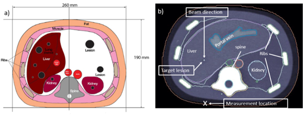
Figure 2. A scheme adapted from the data sheet of the abdominal CIRS phantom (a) shows the dimensions of the phantom and the internal organs. The CT image (b) additionally shows the beam direction, the target lesion and the measurement location.
Download figure:
Standard image High-resolution imageThe phantom mimics human anatomy in the abdominal region using organ surrogates made of different polymers. It was imaged using x-ray CT, magnetic resonance imaging (MRI) and ultrasound. Additionally it includes lesions, one of which was chosen to be irradiated in this experiment to mimic realistic patient treatment. Figure 2(b) shows a CT image of the phantom displaying the target lesion positioned in the liver, the beam direction and the position of the acoustic detector during measurements (measurement location).
To measure the ionoacoustic signal a Cetacean C305X hydrophone was used in axial direction distal to the Bragg peak. According to the data sheet, the hydrophone has a nearly flat frequency response between 20 and 200 kHz and is therefore well suited for the detection of the ionoacoustic signal with a central frequency of approximately f = 80 kHz. The hydrophone was rigidly attached to an ultrasound probe (Interson GP-C01) in a custom made holder, which fixes the relative position of the two devices to each other. The holder was attached to a motorised stage which allowed to alternately drive either device to its measurement location. The lateral offset of the two devices was calibrated in an optoacoustic measurement (see section 2.2). The ultrasound device was operated at a centre frequency of 3.5 MHz and assumes a constant speed of sound of v US = 1.54 mm μs−1 for the ultrasound image generation.
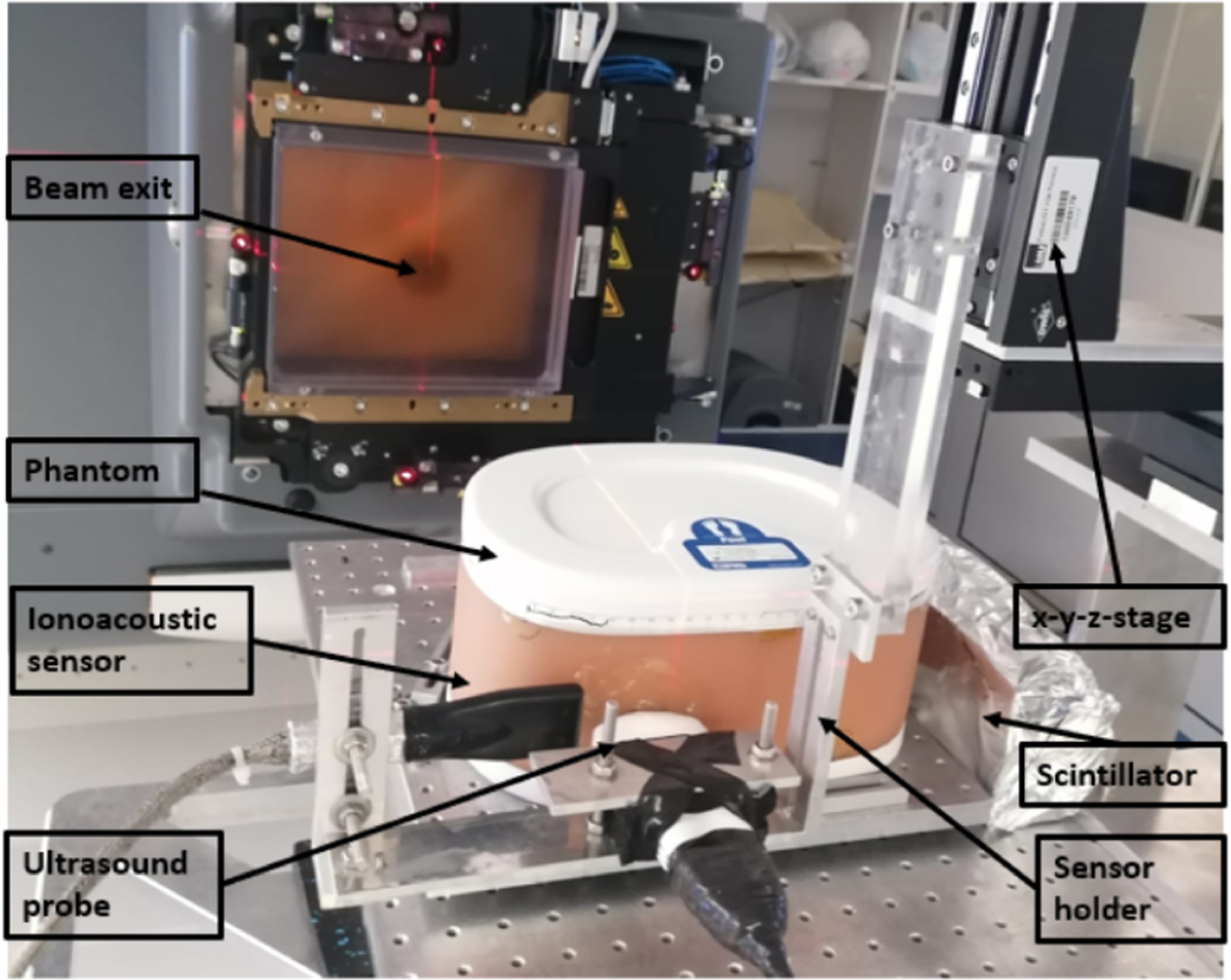
A photo of the experimental setup in the treatment room of the CAL proton therapy centre is shown in figure 3. It depicts the exit window of the proton beam (gantry) with the position of the beam exit marked by the red laser hair cross. The sensors are acoustically coupled to the phantom using ultrasound gel. On the right of the phantom the scintillator of the prompt gamma trigger is shown, which is electromagnetically shielded by aluminium foil.

Figure 3. A photo of the setup shows the beam exit (red hair cross), the phantom, and the custom made holder. The holder is attached to the x–y–z-stage via a transparent PMMA connector. On the right of the phantom the scintillator of the trigger wrapped in aluminium foil can be seen.
Download figure:
Standard image High-resolution imageThe signals from the hydrophone were first amplified using a 40 dB low-noise amplifier (HVA-10M-60-B, FEMTO), followed by a 240 kHz low pass filter and a 5 kHz high pass filter (Thorlabs EF504 and Thorlabs EF115). The signals were then digitised using a 5444D Picoscope (Picotech) at a sampling time of 32 ns and with a 14 bits voltage resolution on a 500 mV range. The data from the ultrasound device was read out directly via USB using the software provided by the vendor.
Due to electromagnetic pulses generated with every proton pulse, it was necessary to electromagnetically shield the ionoacoustic sensor. For this purpose, a piece of aluminium foil was placed between the phantom and the hydrophone and acoustically coupled on both sides with ultrasonic gel. The reduction of the acoustic amplitude at the aluminium foil is negligible due to its small thickness (10 μm) compared to the wavelength ( ) of the ionoacoustic signal.
2.1.2. irradiation planning
FLUKA (Battistoni et al 2007), a Monte Carlo radiation transport simulation engine, was used for the planning of the irradiation. The CT image (see figure 2(b)) of the phantom was transferred into FLUKA using the code built-in capabilities to import DICOM images (Kozłowska et al 2019). The Hounsfield units generated from the CT image were converted into the relevant material parameters such as atomic composition and mass density using the segmentation approach supported by the standard distribution of the code (Kozłowska et al 2019). Beam properties were defined starting from an analytical beam model of the CAL facility (Grevillot et al 2020), tuned to reproduce experimental depth dose measurements in water. The irradiation position was chosen such to mimic a clinical scenario (hepatic lesion in figure 2(b)) while minimising the heterogeneities in the beam and acoustic path. The proton beam energy (126 MeV) was adjusted in silico to position the Bragg peak at the lesion centre.
The experimental setup including the phantom, acoustic detector holder and the motor stage was mounted on the patient couch. During the experiments, the phantom was imaged with ultrasound, and the probe was positioned to have the lesion at the image centre. The phantom was moved laterally using the 6 degree of freedom patient positioning such that the proton beam entered it at the planned position which had previously been marked on the phantom surface. The azimuth angle was determined by aligning the beam with the centre of the ultrasonic probe.
The stopping powers relative to water (SPR) of the phantom materials were derived from water-equivalent thickness measurements of 2 cm thick samples done using a multilayer ionisation chamber (Zebra, IBA) at 150 MeV. The experimental SPRs were used to finely tune the Monte Carlo model. The default FLUKA conversion of HU was substituted by a phantom-specific segmentation accounting for the correct material density and composition as provided by the vendor, and in which the ionisation potential of each material was altered to reproduce the experimental SPR at 150 MeV. The more accurate FLUKA model developed post-irradiation was used as a ground truth to assess the experimental uncertainties.
2.2. Optoacoustic setup
An optoacoustic setup was used to characterise the ionoacoustic detector and calibrate its longitudinal distance to the ultrasonic probe once mounted in the custom made holder. The optoacoustic signals were generated using a 30 W fibre coupled laser diode from Coherent DILAS with a central wavelength of 808 nm. The intensity of the current provided to the laser source was shaped into pulses with a fast modulator FM 45-25 from MPC (Messtec power converter) and a function generator (here: Rigol DG 1022). The laser was focused with a converging lens (f = 10 cm) on a thin (50 μm) black aluminium foil target positioned in a water tank (39 × 39 × 20.5 cm) approximately 4 cm behind the 1 cm thick PMMA entrance wall. The laser is fully absorbed on the target giving rise to an optoacoustic signal emission. A schematic sketch of the setup is shown in figure 4.
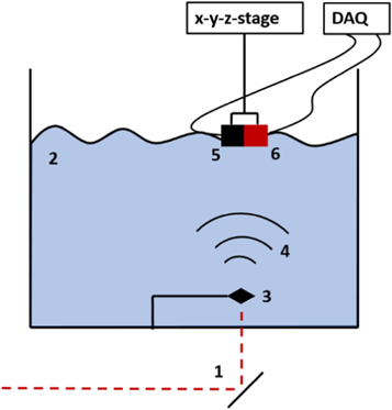
Figure 4. Optoacoustic setup used for calibration measurements. A pulsed laser is reflected at a mirror (1) and enters the water tank (2) through a 1 cm thick PMMA wall before it is absorbed on an aluminium target (3). The optoacoustic wave is emitted (4) and detected by the hydrophone (5), which is rigidly attached to the ultrasound probe (6) in the custom made holder.
Download figure:
Standard image High-resolution imageThe experimental parameters for the calibration measurements were selected to be comparable with the clinical ionoacoustic experiments. A Gaussian pulse of 3.1 μs FWHM was used. The acquisition was triggered from a duplicate of the Gaussian pulse supplied by the function generator and the triggering level was set to 50% of the maximum intensity of the pulse. Only the front side of the hydrophone was immersed in the water (i.e. back side maintained in air) to guarantee the same detector response as for the ionoacoustic measurements with the phantom. Regarding the data acquisition, care was taken to use exactly the same components as in the ionoacoustic measurements to exclude any additional electrical delays in the optoacoustic signals due to electronics such as additional filters or amplifiers.
For the calibration, it is necessary to ensure that the optoacoustic measurement and an ultrasound image are recorded on the beam axis. For this purpose, the hydrophone was scanned in both dimensions lateral to the beam axis in 1 mm steps and optoacoustic signals with identical conditions were recorded at each position. The position on the beam axis along a scan direction was determined as the position that achieves maximum optoacoustic amplitude, which was determined with a parabolic fit. The axial measurement position for the ultrasound device was determined by moving the ultrasound device iteratively in millimetre steps until the aluminium target was visible at maximum intensity and symmetrical to the central axis of the ultrasound device (see figure 12). The longitudinal distance between the sensors and the aluminium foil target was chosen to match the expected distance to the Bragg peak during the ionoacoustic measurements (≈65 mm). The optoacoustic setup with the hydrophone positioned on the beam axis was also used to characterise the hydrophone with respect to its total impulse response (TIR) (see section 3.1.2).
2.3. Signal-processing of ionoacoustic measurements
In the evaluation process, the signals of consecutive proton pulses are averaged accumulating a total dose proportional to the number of averages. The total dose of an n-fold averaged measurement can thus be calculated by D = n × 2.40 cGy. The resulting n-fold averaged measurements M(t) are then filtered with a correlation filter utilising a simulated filter template F(t) (Schauer et al 2022). The template reflects the temporal structure of the expected ionoacoustic signal (Turin 1960). A correlation filter is mathematically designed to maximise the SNR of a raw measurement containing a signal of known shape (Turin 1960). The output of the filter is a correlation function which is often called a measure of similarity because it maximises at the point where the maximum similarity between measurement and template is found. For discretised input signals the correlation function CM,F (τ) reads as

The variable τ describes the time shift between the template and the measurement. The denominator consist of the total signal energy contained in the measurement (Σt M2(t)) and template (Σt F2(t)), respectively and ensures correlation coefficients between −1 and 1.
The templates F(t) used for the filtering process are based on the theoretical derivation of Jones et al (Jones et al 2016, 2018). It represents the expected pressure at the detector at time t, which is given by the convolution of a spatial contribution Pδ (t), a temporal contribution determined by the derivative with respect to time of the temporal heating function Ht (t), and a second convolution with the total impulse response of the ionoacoustic detector TIR(t).

Ht
(t) is given by the normalised beam current  in units of [s−1] and Pδ
(t) is given by a spherical surface integration over the dose D(R, θ, ϕ) deposited by the proton beam, given in the coordinate system of the detector (R, θ, ϕ)(see figure 6(a)).
in units of [s−1] and Pδ
(t) is given by a spherical surface integration over the dose D(R, θ, ϕ) deposited by the proton beam, given in the coordinate system of the detector (R, θ, ϕ)(see figure 6(a)).

Here, Γ(R, θ, ϕ) is the dimensionless Grüneisen parameter describing the conversion of heat to pressure (Mausbach et al 2016) and ρ(R, θ, ϕ) the mass density of the material in which the dose D(R, θ, ϕ) is deposited. The distance between the an arbitrary point within the source and the detector is described by R = vs t, with vs being the speed of sound of the propagation medium.
3. Results
The results section of this manuscript is divided into three parts. The first part describes the raw signals and how the used correlation filter improves the SNR thus making signals visible at clinically relevant doses. The second part presents the extraction of a robust time of flight and demonstrates the high accuracy in detection of a relative range shift originating from a change in the energy of the proton beam. In the third part, it is shown, how the Bragg peak location obtained from a ionoacoustic signal can be assigned to a location in an ultrasound image by means of an optoacoustic calibration measurement.
3.1. Evaluation process of the ionoacoustic measurements
3.1.1. Unfiltered ionoacoustic measurements
Using the setup described in figure 3, ionoacoustic signals from 1200 consecutive proton pulses were individually recorded. As for each individual measurement a stable trigger was provided by the prompt-gamma-signal (see figure 1), the total number of protons taken into account and correspondingly the dose could be determined by the number of measurements averaged. Figure 5 shows the raw (i.e. unfiltered) ionoacoustic measurements including all 1200 averages (a) and one example of 50 averages (b).
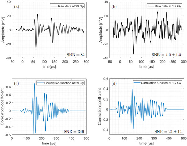
Figure 5. Raw ionoacoustic signals with 1200 averages or 29 Gy total dose in the Bragg peak in (a) and one example of a signal containing 50 averages or 1.2 Gy in (b). The corresponding correlation function after filtering the raw signals with the filter templates (see figure 7(b)) are plotted in (c) and (d), respectively.
Download figure:
Standard image High-resolution imageIn figure 5(a), the high number of averages and the associated low noise level allow the identification of two individual signals separated in time. The first signal, the so-called direct signal, starts at about 50 μs and is caused by the sound waves travelling from the Bragg peak to the sensor in a straight way. In addition, another signal, the so-called window signal, is also visible and starts at about 130 μs. This signal is generated by the entry of protons into the abdominal phantom. This signal is likely to be overlaid by echoes of the direct signal or other secondary signals which dominate the signal after 150 μs . If not further specified in the following 'the signal' always refers to the direct signal, which is the most interesting one since it contains the information of the distance between the Bragg peak and the sensor. In contrast to the high SNR measurement in (a), the low averaging number of 50 averages displayed in (b) causes a substantially higher noise floor making the signals hardly distinguishable from pure noise.
3.1.2. Filtering process of the raw measurements
The noise level in the measurements shown in figure 5(a) and (b) was reduced by a correlation filter. The filtered signals (correlation functions) plotted in figure 5(c) and (d), respectively, are obtained after correlating the raw measurements from (a) and (b) with a simulated filter template. The template reflects the temporal structure of the expected ionoacoustic signal as accurately as possible and are obtained in this work as a hybrid between simulation and measurement. The generation of the three components (see equation (2)), which are necessary for the generation of a complete template, is described below.
The 3D dose distribution of the proton beam D(R, θ, ϕ) was simulated using TOPAS (Perl et al 2012), a Monte Carlo dose engine based on Geant 4. 9.4 × 10⁶ protons were simulated in a water phantom and the dose was read out in a cartesian scoring of 200 μm. The dose was subsequently transferred into MATLAB and multiplied with the mass density of the material (water) and the Grüneisen parameter for water (Γ = 0.12 at 21°C (Wang and Wu 2012)). The spherical surface integration (see figure 3) was numerically evaluated using cubic interpolation starting from a voxel positioned 65mm distal to the Bragg peak marking the expected sensor position. The resulting Pδ (t) is initially still a function of location, which can be transcribed to a function of time under the assumption of a speed of sound (vs = 1.50 mm μs−1). The calculation of Pδ (t) is illustrated in figure 6 for a 2D cut of the 3D dose distribution (colour coded).
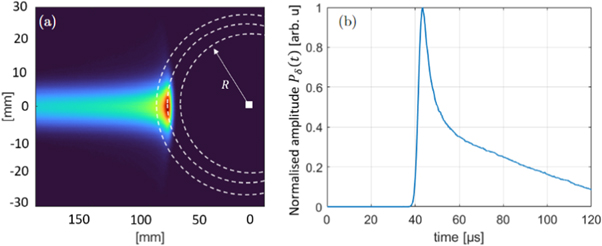
Figure 6. (a) shows a cross section of the input dose distribution (colour coded) with the sensor position marked as a white square. All pressure contributions p0 = Γ(R, θ, ϕ)ρ(R, θ, ϕ) D(R, θ, ϕ) located on a sphere (white dotted lines) arrive at the detector at the same time t = R/vs where they sum up to form Pδ (t) (b).
Download figure:
Standard image High-resolution imageThe sensor position is marked by the white square (a). All pressure contributions associated with the corresponding dose distributions by p0 = Γ(R, θ, ϕ) ρ(R, θ, ϕ) D(R, θ, ϕ) located on a sphere (circle) indicated by the white dotted lines arrive at the detector at the same time t = R/vs where R is the distance to the detector and vs is the speed of sound assumed for the calculation. This time dependent generic pressure is given by Pδ (t) (figure 6 (b)). It is plotted with a normalised amplitude as the amplitude of Pδ (t) has no effect on the resulting filtered signals. It is consequently not necessary to know the Grüneisen parameter or the mass density of the irradiated medium precisely as long as they are constant in the region around the Bragg peak. The calculation of Pδ (t) allows to find the time point t in Pδ (t), which corresponds to a certain point in the dose distribution characterised by its distance to the sensor x = vs t. For this particular irradiation geometry it was found that the distance between the Bragg peak and the sensor maps to a time of flight which is given by the maximum of Pδ (t). The Bragg peak was chosen for simplicity reasons only, similarly other characteristic points of the dose distribution, like the 80% fall-off of the Bragg peak, can be found in Pδ (t) using the same method. Pδ (t) is subsequently convolved with the temporal derivative of the temporal heating function emulating the expected temporal heating function from the synchrocyclotron at CAL, (Gaussian with FWHM=3.1 μs), and the TIR(t) in order to obtain a complete simulation of the signal F(t) according to equation (2).
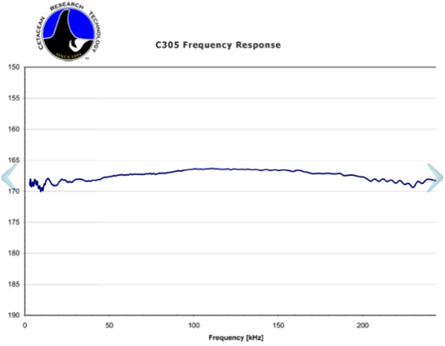
The frequency response of the hydrophone as given on its data sheet (see figure 15, appendix) is only valid for its usage when completely submerged in water. Since the hydrophone in this experiment was operated with air as a backing material, this changes the impulse response and frequency response drastically. Thus, the TIR(t) was experimentally measured using the optoacoustic setup (see section 2.2). This measurement ensures that acoustic reflections on air and internal structures of the hydrophone are also included in the TIR. To measure the TIR of the hydrophone, a rectangular, long (30 μs) laser pulse was generated using the function generator. For the first 30 μs of the measured TIR it can thus be assumed that the causing temporal heating function Ht (t) reduces to a heavyside step function and its temporal derivative reduces to a delta-function. The pulse duration of 30 μs ensures frequencies as low as approximately 30 kHz to be correctly included in the TIR. Lower frequency components with a period of more than 30 μs might not be perfectly measured using this setup, however these components have a negligible contribution to the ionoacoustic signal and could not be measured using the optoacoustic setup as presented here, since secondary signals originating from the PMMA wall are expected to arrive approximately 30 μs after the primary signal distorting the TIR from this time point onwards. Note that the distance between the aluminium foil target and the hydrophone was chosen to match approximately the expected distance between the Bragg peak and the hydrophone in the subsequent ionoacoustic measurements. This ensures the TIR to be as well adapted to the ionoacoustic measurements as possible. However, as the spherically expanding pressure wave from the aluminium foil target is approximately flat in the region of the hydrophone, it is expected that the TIR is robust against small changes in this distance especially to distances larger than the one used.
Additionally, since all photons are absorbed on the thin aluminium foil with a thickness of d = 50 μm being much smaller than the wavelength of the acoustic signal (λ ≈ 1.9 cm), Pδ (t) reduces to Pδ (t) = δ(t). The expected signal (for the first 30 μs) can thus be written as:

The resulting total impulse response (TIR(t)) of the detector is shown in figure 7(a). The first pronounced maximum of the TIR(t) is due to the incoming pressure wave, followed by two smaller minimums which are likely due to reflections of the incoming pressure on internal structures of the hydrophone. Because of the high impedance change on the back of the hydrophone the pressure wave is almost completely reflected at the air surface causing a second very pronounced maximum.

Figure 7. Characterisation of the Cetacean 305X hydrophone in terms of its TIR(t) (a). Panel (b) shows the obtained template F(t) (orange line), which is obtained by convolution according to equation (2). Pδ (t) (blue line) originating from the dose deposition of the 126 MeV proton beam was convolved with the temporal derivative of the heating function (Gaussian with FWHM = 3.1 μs) and the TIR(t) from panel (a).
Download figure:
Standard image High-resolution imageThe template is shown in figure 7(b) (orange) together with Pδ (t) (blue), whose simulation was discussed in the context of figure 6. Starting with Pδ (t), the template was obtained by convolution according to equation (2). The temporal shift between Pδ (t) and the template originates from the numerical cut-off points of the temporal heating function and the TIR(t) defining their respective start and end. This shift has therefore no direct physical meaning, however it is important for the further course of this manuscript that this temporal shift is fixed. Given the position of the template in time, the corresponding position of Pδ (t) in time is thus known from this convolution process.
3.1.3. Correlation function results
After correlating the raw measurements from figure 5(a) and (b) with the filter template (see figure 7 (b), orange line), the correlation functions plotted in figure 5(c) and (d) are obtained. The increase in signal quality achieved by the correlation filter is particularly evident in the signal with 50 averages (see figure 5(b) and (d)). In contrast to the raw measurement, the signal position (at 150 μs) is clearly visible in the correlation function and the maximum of the correlation function is at least two times larger than the amplitudes of the noise as visible for t < 130 μs. The signal quality of both, raw measurements and correlation functions are quantified using an SNR according to (Schauer et al 2022). For the signals containing 50 averages the given SNR-values (see values in the figure) are mean values as the SNR fluctuates depending on which 50 averages were considered. This fluctuation is quantified by the standard deviation of the individual measurements. For the signals containing all 1200 averages no statistical uncertainty in the SNR can be given as there is only one measurement.
A key feature of the correlation function is the fact that the maximum position of the correlation function can be used to determine the signal position in the measurement. It is used to match the template to a position in the measurement, where it best matches the signal shape. For a measurement and a template which are of the same duration (like in this work) the shift that has to be applied to the original template in order to match the template to the measured signal can be calculated by subtracting the length of the template from the correlation peak position (see figure 5(c), (d)). The length of the measurement and the template is equal to 10 000 samples or 320 μs. Note, that the template in figure 7(b) only shows a section of the template for better visibility. The matching procedure is illustrated in figure 8, which shows the raw measurement as displayed in figure 5(a) (black) together with the matched template (orange).

Figure 8. Using the correlation function, the simulated template (orange) can be matched to the measurement (black). From the template generation the relative position of the template and Pδ (t) is known and additionally plotted (blue). The trigger signal is plotted in purple.
Download figure:
Standard image High-resolution imageThe relative position of the template to the measurement was determined from the maximum position of the correlation function (see figure 5(c)) between measurement and template. From the matched template position, the position of Pδ (t) (blue) is also known since it was fixed in the template generation (see figure 7). Additionally the 1200-fold averaged trigger signal is shown (purple).
While the position of Pδ (t) or more precisely the position of its maximum, which will be used for the evaluation process, is to be calibrated in terms of absolute time of flight it already allows for the determination of a range difference between two proton beams from their respective ionoacoustic signals. The position of Pδ (t) as obtained from the correlation and matching procedure is very robust against noise since it depends on the correlation peak position and therefore the whole signal structure rather than a single point in the signal.
3.2. Range variation measurements
The correlation analysis was performed for ionoacoustic signals generated by protons of energy E1 = 126 MeV (Figure 9, black) and E2 = 127 MeV (figure 9, orange) measured on the CIRS phantom using the setup shown in figure 3. Both signals are shown for a dose deposition of 29 Gy at the Bragg peak (1200 averages). In addition, figure 9 shows the corresponding Pδ (t) for both energies (dotted lines), which are obtained after the correlation and matching procedure (see figure 8). The temporal difference of the Pδ (t)-peaks (Δ tV ) is used to assign a time of flight difference between both signals and was found to be ΔtV = 1.02 μ s ± 0.10 μs. The subscript V stands for 'variation' and the indicated uncertainty is deduced later in this section.

Figure 9. Raw ionoacoustic signals corresponding to two different proton energies, namely 127 MeV (orange, solid) and 126 MeV (black, solid). For both energies the corresponding positions of Pδ (t) (dotted) is shown and their temporal offset is evaluated to be ΔtV = 1.02 μs ± 0.10 μs .
Download figure:
Standard image High-resolution imageThe speed of sound in the phantom in the irradiated region of the phantom (liver) is known from the manufacturer to be vL = 1.54 ± 0.01 mm μs−1. Assuming that both proton beams stopped in the liver, which is a valid assumption given the spatial extend of the liver from figure 2, a spatial distance between the Bragg peak of the 127 MeV protons and the 126 MeV protons is calculated:

It should be emphasised here that the difference in time of flight could have been directly read from the raw signals when using these high dose measurements. However, the temporal difference between the two signals strongly depends on the point within the signal that is used for comparison. This jitter increases when decreasing the number of averages (see figure 5 (b)). In comparison, the position of Pδ (t) as resulting from the correlation analysis is much more robust against noise. This is quantified in figure 10 showing the analysed peak-positions of Pδ (t) for measurements at different doses for the 126 MeV and the 127 MeV beam. The ranges are given relative to x0 defined by the peak-position of Pδ (t) for the 126 MeV protons measured with 29 Gy. Figure 10 shows the dose dependent scattering of the data starting on the right at one measurement containing 1200 averages down to 24 measurements containing 50 averages each. For both energies the scattering of the data increases with decreasing dose due to the increasing noise floor. The offset of the symbols in figure 10 at a dose of 29 Gy is given by the deviation in range of the two corresponding proton beams (1.57 mm), which was evaluated in figure 9. A quantification of the scattering of the 24 measurements at 1.2 Gy each is given in table 1.

Figure 10. Evaluation of the statistical error for E1 = 126 MeV (black crosses) and E2 = 127 MeV (orange circles) as a function of dose between 1.2 Gy and 29 Gy. The offset of the two values at D = 29 Gy is given by the distance in range of the corresponding proton beams.
Download figure:
Standard image High-resolution imageTable 1. Quantification of the scattering of the evaluated Pδ (t)-peak position for a dose of 1.2 Gy and energies of 126 MeV and 127 MeV.
| E = 126 MeV | E = 127 MeV | |
|---|---|---|
| standard deviation σ [mm] (μs) | 0.52 (0.34) | 0.46 (0.30) |
maximum deviation  [mm] (μs) [mm] (μs) | 1.53 (0.99) | 1.1 (0.71) |
| Number of deviations >1 mm | 1 | 1 |
It shows that the standard deviations are below 1 mm with 0.52 mm for the 126 MeV and 0.46 mm for the 127 MeV case. The two standard deviations are used to calculate a standard error of the mean:


The SEM-values are the expected standard deviation of the measurement containing all 1200 averages if it was repeated multiple times. Using the SEM-values an error can be calculated for the range difference calculation of the two energies as it was performed in equation (5). Here, the individual jitter of the maximum position of Pδ (t) (SEM) and the uncertainty of the speed of sound contribute. The range difference is thus equal to ΔR = 1.57 ± 0.14 mm which agrees with the value from TOPAS simulations (1.60 mm) within the margins of the measurement uncertainty. This result shows that it is possible to determine a range shift between two proton beams from their corresponding ionoacoustic signal for clinically relevant conditions with sub-millimetre accuracy.
3.3. Bragg peak localisation
The measurement of range variations from the previous section can already be used for clinical applications, for example to compare the measured ionoacoustic signal to simulations as expected from the irradiation plan. However, the evaluation process as presented was based on the assumption that both beams stop in the same tissue of known speed of sound. Ionoacoustics additionally offers the possibility of a Bragg peak localisation. For this, the ionoacoustic measurement must be calibrated once. An optoacoustic setup (see figure 4) was used for this purpose. In the following, the calibration of the ionoacoustic sensor is presented to localise the Bragg peak relative to the ionoacoustic sensor before, in a second step, the calibration is adapted so that the Bragg peak can be localised relative to the anatomy, which is obtained by an ultrasound image.
3.3.1. Calibration of the ionoacoustic sensor using optoacoustics
The calibration of the ionoacoustic sensor is necessary in order to convert a measured time of flight obtained from the maximum position of Pδ (t) to a location relative to the ionoacoustic sensor. The optoacoustic setup is suitable for the calibration process as the location of the origin of the optoacoustic signal is known as it is confined within the black aluminium foil target. The calibration is specifically designed for the synchrocyclotron at CAL. In order to make the optoacoustic calibration suitable for the evaluation of the ionoacoustic measurements, the parameters which influence the shape of the ionoacoustic signal (see equation (2)) were reproduced as precisely as possible in the optoacoustic setup.
Additionally to the setup parameters, identical signal-processing was applied for the optoacoustic calibration measurement. This includes the generation and the matching of a template for which it was ensured to use the numerically identical temporal heating function and TIR(t). In contrast to the ionoacoustic measurements, the energy distributions and therefore also Pδ (t) was assumed to be delta-shaped as all photons are absorbed on the thin (50 μm) aluminium foil target. The evaluation process for the optoacoustic measurement is illustrated in figure 11.
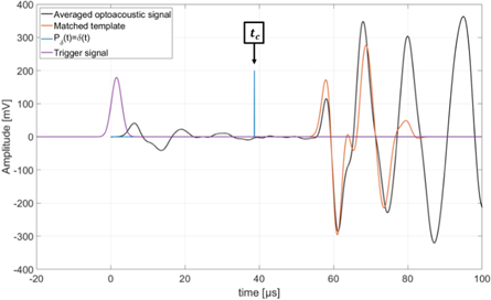
Figure 11. Optoacoustic signal generated by the laser absorption on the aluminium foil target (black). The optoacoustic template (orange) is matched to the signal and the position of Pδ (t) = δ(t) is marked as the calibration time tc . Additionally the trigger signal (purple) is plotted. The starting time t = 0 s is chosen to match the 50% mark of the rising flank of the Gaussian pulse.
Download figure:
Standard image High-resolution imageThe template (orange) generated for the evaluation of the optoacoustic signal (black) is matched to the signal using the corresponding correlation function and the position of Pδ (t) = δ(t) (blue) relative to the template is known from the template generation. This time is defined to be the calibration time tc . This time has no direct physical meaning and is in particular not equal to the time of flight of the acoustic signal from its source at the aluminium foil target to the hydrophone. However, the calibration time enables a comparison to ionoacoustic measurements. Note that a comparison between optoacoustics and ionoacoustics is not self-evident as for the raw signals the different contributions from the different Pδ (t) cause different signal shapes. The comparison is only made possible by the calculation of the position of the individual Pδ (t) as within Pδ (t) the corresponding point of the dose deposition is known (see figure 6).
In order to finalise the calibration, the calibration time was complemented with a calibration distance. This calibration distance is given by the distance between the acoustic source, namely the aluminium foil target, and the ionoacoustic sensor. This can be physically measured using, for example, a caliper. The temporal difference between the calibration time tc and the time of flight extracted from the maximum position of Pδ (t) of an arbitrary ionoacoustic measurement (tM ) can now be converted to a distance between the calibration location xc and the Bragg peak location (xBP). In particular:

Here, xc and tc are obtained from the calibration, vc is the speed of sound of the water used for the calibration process and vM is the average speed of sound traversed by the ionoacoustic signal. While the speed of sound of the water used for the calibration process can be measured with high precision, the speed of sound of tissue is generally not known with sufficient accuracy to perform range verification in a clinical context. Additionally, the distance between the hydrophone and the Bragg peak is an incomplete information regarding a range verification process. Rather, it is desirable to know the Bragg peak position relative to the anatomy of the patient instead of its position relative to the sensor. This can be achieved by the combination of the time of flight obtained from a ionoacoustic measurement with a medical ultrasound image.
3.3.2. Bragg peak localisation in an ultrasound image
The combination of the ionoacoustic measurement with an ultrasound image requires a slightly modified calibration with regard to the calibration distance while the calibration time stays unaltered as presented in the previous section. Instead of measuring the distance to the aluminium foil target physically, the calibration location is obtained from an ultrasound image taken at the same measurement location as the optoacoustic calibration measurement. This calibration thus maps the calibration time to the location in the ultrasound image where the aluminium foil target is displayed, which is called the calibration location xc . This ultrasound image is shown in figure 12.
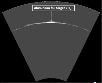
Figure 12. Ultrasound image of the aluminium foil target defining the calibration location xc . The ultrasound image is recorded at the same lateral position as the optoacoustic measurement used for the extraction of the calibration time tc (see figure 11).
Download figure:
Standard image High-resolution imageFor the calibration process neither the absolute distance to the Aluminium foil target nor the speed of sound of the water matters since they are equal for both devices given that both devices measure on the beam axis. A higher or lower speed of sound of the water changes the arrival time of the optoacoustic signal but simultaneously stretches or compresses the ultrasound image since the ultrasound probe assumes a constant speed of sound of vUS = 1.54 mm μs−1 for image generation. It has to be assumed that the dispersion in the frequency range between the acoustic signals (80 kHz) and the ultrasound probe (3.5 MHz) is negligible, which has been shown for water and haemoglobin solutions mimicking soft tissues (Treeby et al 2011).
This calibration is used to transfer the time of flight obtained from the maximum position of Pδ (t) of an arbitrary ionoacoustic measurement (tM ) to the ultrasound image. Assuming the case, where by chance this maximum position tM coincides with the calibration time tc , then the corresponding point within the ultrasound image would be the calibration location xc . Accordingly, a temporal difference between tM and tc (tM − tc = ΔtL ) can be converted to a distance between xc and the point of interest using the default speed of sound considered for US image generation vUS .

Here, ΔxL is the difference between the calibration location and the point of interest as displayed in the ultrasound image and the subscript L is short for 'localisation'. Note, that using this method the point of interest is the position of the maximum of Pδ (t), which, for the given irradiation geometry, coincides with the Bragg peak position (see figure 6). The evaluation of the temporal difference between tc and tM evaluated from the ionoacoustic measurement using 126 MeV protons is illustrated in figure 13.

Figure 13. Pδ (t) obtained from the ionoacoustic measurement using 126 MeV protons and a dose of 29 Gy (black). Additionally the calibration time is plotted in blue.
Download figure:
Standard image High-resolution imageThe calibration time is indicated in blue and Pδ (t) as evaluated from the ionoacoustic measurement with 126 MeV protons (see figure 8) is shown in black, while its maximum position is indicated by the black dashed line. Their temporal difference is calculated to be ΔtL = 0.80 μ s ± 0.07 μs, where the indicated uncertainty was calculated in equation (6). This temporal difference is converted to a difference in distance according to equation (9) yielding a spatial offset between the Bragg peak and the calibration location of ΔxL = 1.23 ± 0.10 mm. This spatial offset is used to mark the Bragg peak position in the ultrasound image showing the irradiated region of the phantom using the integrated scale bar intrinsic to every ultrasound image (see figure 14).
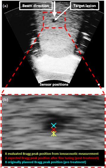
Figure 14. The ultrasound image showing the irradiated region of the CIRS phantom highlighting the target lesion (a). Additionally the beam direction and the sensor positions are indicated. The red dashed line shows an inlay which is zoomed in (b). It shows the target lesion with the originally planned Bragg peak position (blue), the expected Bragg peak position after fine tuning the SPR (see section 2.1.2) and the evaluated Bragg peak position (yellow) with the error bars indicating the standard deviation found for a dose of 1.2 Gy.
Download figure:
Standard image High-resolution imageThe same argument as in the calibration holds: While there are a variety of different speeds of sound present in the abdominal phantom which each affect the arrival time of the ionoacoustic signal, the same speeds of sound affect the image generation from the ultrasound probe leading to a stretched or compressed display of the involved media in the ultrasound image. The Bragg peak position can thus be marked as if it would be visible in the ultrasound image, using the ionoacoustic sensor as a low-frequency extension of the ultrasound probe. The ultrasound image including the evaluated Bragg peak position is shown in figure 14.
Panel (a) shows the whole ultrasound image indicating the beam direction, the target lesion and the sensor position. The contrast of the image has been increased to make the target lesion more visible. This is the reason why the image looks overexposed in certain areas. The region indicated by the red rectangle is enlarged in (b) showing the evaluated Bragg peak position from the ionoacoustic measurement (yellow). Additionally, the originally planned Bragg peak position (blue) and the expected Bragg peak position after fine tuning the SPR within the irradiation planning process (red) are marked. The error bar in the measurement is given by the standard deviation of the individual measurements at 1.2 Gy (0.52 mm).
Assuming that the expected Bragg peak position (red) is the ground truth, there is a deviation of approximately 1.0 mm between the expected Bragg peak position and the measured Bragg peak position, which cannot be entirely explained by the statistical uncertainty of the measurement. Nonetheless a Bragg peak localisation with an accuracy of 1.0 mm relative to the anatomy is a substantial reduction to the typical range uncertainties in proton therapy, which are between 1 and 8 mm depending on the tumour (Paganetti 2012).
4. Discussion
This paper has demonstrated that ionoacoustics has the potential to perform measurements regarding a range variation of the proton beam with a statistical uncertainty of σ = 0.5 mm. In addition it has been demonstrated that it is possible to localise the Bragg peak position relative to the ionoacoustic sensor and to integrate the Bragg peak position into an ultrasound image of the irradiated region. The measured Bragg peak position shows a non-negligible deviation of about 1.0 mm compared to the expected Bragg peak position expected from irradiation planning in the abdominal phantom. Thus, even if the deviation is completely attributed to the uncertainty in the measurement, it demonstrates, that the goal in online Bragg peak monitoring with 1.0 mm uncertainty has been achieved.
Discussing the 1.0 mm deviation of measured and planned Bragg peak position in detail, one has to consider both, the systematic errors in irradiation planning and systematic errors in the measurements. The uncertainty in the planned Bragg peak position is much lower than in a typical clinical scenario, as the materials have been carefully characterised with respect to their stopping power. However, also considering possible misalignments of the phantom relative to the beam, the planned Bragg peak position may be subject to a systematic uncertainty of 1.0 mm. In this case, the ionoacoustic measurement could subsequently be used to adapt the irradiation plan and reduce the proton energy correspondingly.
On the other hand, however, the observed difference in Bragg peak position may be attributed to systematic errors or inaccuracies in the parameters in data evaluation. The major contribution may originate from the trigger signal as it was found that the width of the Gaussian slightly depends on the position of the trigger detector as well as its input voltage. An improved trigger and the associated measurement of the pulse shape for future experiments or clinical applications is solvable. The use of a photodiode instead of the photomultiplier used for processing the prompt gamma signal promises a more stable trigger reading, as the photomultiplier reacted too sensitively to the large number of prompt gammas. For a reduction of systematic errors, the trigger signal and the whole pulse shape is of great importance as it defines the starting point of the measurements and is additionally used during the calibration process. During calibration, the greatest possible accuracy must be ensured, as a systematic error in the calibration will be reflected in all subsequent ionoacoustic measurements. However, it should be emphasised that a successfully calibrated instrument can be used without restriction, as the calibration is independent of the irradiation or measurement location and therefore does not need to be renewed regularly.
To exclude all systematic errors in the planned dose profiles as well as in the analysis of the ionoacoustic signals, additional experiments are needed in the future to compare the ionoacoustic measurement with a measured dose profile using, for example, an dosimetric phantom. Such a ground truth measurement makes it possible to further reduce the systematic uncertainties but will also replace the optoacoustic calibration measurement.
Regarding a possible clinical application the presented method comes with the additional advantage that the evaluation process can be performed in real time providing the position of the Bragg peak in an ultrasound image of the patient recorded at the time of irradiation. During the evaluation of the distance between the Bragg peak position and a reference point in the ultrasound image (dUS ) care must be taken that measuring distances in an ultrasound image requires the knowledge of the real speed of sound (vreal) of the media between the Bragg peak and the reference point. The actual physical distance can be calculated from an ultrasound image using the ratio of the real speed of sound to the default speed of sound of the ultrasound probe vUS .

Uncertainties in the calculation of dreal are mostly attributed to the imprecise knowledge of vreal within the body. As this uncertainty is linearly dependent on the measured distance dUS it is advisable to choose a reference point within the ultrasound image which is as closely positioned to the Bragg peak position as possible. Ideally, this reference point would be the lesion itself.
In this manuscript the location of the Bragg peak was evaluated for simplicity reasons rather than other characteristic points of the dose distributions like the 80% fall-off which is arguably more commonly used to define the range (Carabe et al 2012). However, using the presented method, the dose distribution and the corresponding Pδ (t), which is used for the evaluation process, is fixed within simulation (see figure 6). It is thus straightforward to determine the position of other characteristic points like the 80% fall-off or even the whole dose distribution within the ultrasound image. However, it must be emphasised, that the shape of the dose distribution itself is not actually measured but rather the a priori knowledge about the shape of the dose distribution is used (in the template) to determine its position in the ultrasound image.
Although the used dose in this work of 1.2 Gy is lower than the typical dose administered in a treatment fraction (2 Gy), further dose reduction is necessary. In state of the art proton therapy, it is common practice to irradiate the tumour from different directions, which means that it is conceivable that no single lateral pencil beam contains the full dose of 2 Gy. A promising starting point for dose reduction without a reduction in signal quality is the used hardware. This includes amplifiers, filters, data acquisition, but above all the used hydrophone.
In recent studies from 2022 (Sueyasu et al 2022) and 2023 (Caron et al 2023), ionoacoustic signals could even be measured from single pulses using an optical hydrophone and/or piezoelectric ones (Olympus V389-SU (Caron et al 2023), Olympus V391-SU (Sueyasu et al 2022)). The comparability with the cited studies is only valid to a limited extent due to differences in the experimental design. In particular, it must be mentioned that the studies (Sueyasu et al 2022) and (Caron et al 2023) both use a water phantom and a substantially higher beam current (more than 4-fold) than in this study. It has already been shown that a higher instantaneous beam current contributes to a higher SNR at the same number of protons or dose (Schauer et al 2022), respectively. Nevertheless, the cited papers suggest that the Cetacean hydrophone used in this study is not ideal for the detection of ionoacoustic signals. While a more sensitive detector would reduce the dose required for the evaluation process, this does not change the main points of this work, namely the determination of a robust point for the time-of-flight extraction as well as its calibration and the associated transfer into an ultrasound image.
In a 2021 published study by Patch et al using the same CIRS abdominal phantom and a combination of four transducers attached to an ultrasonic probe, ionoacoustic signals measured at a dose deposition of <0.5 Gy could be used for the evaluation process (Patch et al 2021). In the work of Patch et al the measured ionoacoustic signals were compared with acoustic signals simulated on the basis of the treatment plan. A deviation of the Bragg peak position from the treatment plan was assessed using the time of flight difference between the simulated and the measured signals. Compared to our work, this comes with the disadvantage that the sensor position as assumed in the simulations has to be replicated with high accuracy in the physical setup. In addition, this evaluation method requires the speed of sound of the phantom materials to be known. For the CIRS abdominal phantom, these are specified by the manufacturer but it cannot be assumed that this also applies to human patients. In contrast, the combination of the hydrophone and the ultrasound probe as demonstrated in this study works independently of the speed of sound as long as it is ensured that it is equal for both devices (i.e same measurement position and negligible dispersion (Treeby et al 2011). While the integration of the time of flight obtained from a ionoacoustic measurement into an ultrasound image is no novelty in itself (Assmann et al 2015, Patch et al 2019), it has so far only been demonstrated using the same sensor for the detection of the ionoacoustic measurements and the generation of the ultrasound image (Patch et al 2019). This method requires that the central frequency of the sensors are suited both for the detection of ionoacoustic signals and ultrasound image generation. For clinical applications, this condition imposes limitations on the quality of the ionoacoustic signal or the ultrasound image since the central frequency of the ionoacoustic signal for clinical proton energies (300kHz–30 kHz for energies between 50 MeV and 250 MeV (Schauer et al 2022)) deviates substantially from the optimal frequency for ultrasound imaging (several MHz). Thus one very important component of this work is the combination of the low-frequency ionoacoustic detector with the high-frequency ultrasound probe via the calibration using the optoacoustic setup.
Compared to other range verification methods the integration within an image of the patients anatomy is a major advantage while one limitation of ionoacoustics is the requirement of a pulsed beam with a pulse duration adapted to the energy (Schauer et al 2022). In contrast, range verification using prompt-gamma-emissions can work independently of the underling pulse structure of the beam. Regarding a comparison of the precision of the two methods, a recent study using state of the art prompt-gamma-spectroscopy (Hueso-González et al 2018) found a similar statistical uncertainty of σ ≈ 0.50mm for 12 independent measurements of the range error of clinical proton beams in a water phantom. The range error was evaluated as the difference between the measurement and the prediction obtained from the treatment plan. For the assessment of the range error, 14 independent pencil beams differing in lateral position and energy were combined in a merging region. As each pencil beam at the distal end delivered approximately 1.2 × 10⁸ protons, the total number of protons (approximately 1.7 × 10⁹) exceeded the number of protons used in this study (4.7 × 10⁸) by a factor of 3.5.
5. Conclusion
This paper has demonstrated the potential use of ionoacoustics as a range verification method for proton or ion beam irradiation. It has been shown how a time of flight can be robustly extracted from the ionoacoustic signal and subsequently used to measure range variations or localise the Bragg peak relative to the anatomy of the irradiated abdominal phantom by combining the ionoacoustic signal with a medical ultrasound probe. For this experiment, clinically relevant irradiation conditions were used in terms of energy (126 MeV protons) and dose (1.2 Gy). At this dose, the usage of a correlation filter enables a noise robust time of flight determination from the ionoacoustic signals with a statistical precision of σ ≈ 0.5 mm. The systematic deviation between the Bragg peak position obtained from the ionoacoustic measurement and the one expected from a finely tuned irradiation planning process accounting for a careful characterisation of the irradiated materials is approximately 1 mm. This high accuracy offers the potential to reduce the size of the PTV and thus increase sparing of healthy tissue due to the smaller margins around the CTV in the longitudinal direction. Critical organs behind the tumour may be spared more effectively, which would reduce side effects caused by irradiation of healthy tissue and potentially enable the realisation of more beneficial irradiation geometries, which are currently hindered because of the large range uncertainty.
Acknowledgments
The authors acknowledge the financial support by DFG (Project NR: 403225886), the EU project Radiate, the Center for Advanced Laser Applications (CALA) and ATTRACT project funded by the EC under Grant Agreement 777222. The authors further acknowledge the help of Katrin Schnürle and Pratik Dash who have contributed to the accuracy of the irradiation planning. Additionally, the authors acknowledge the help of Prof Anatoly Rosenfeld, Dr Matthias Würl and Dr Jona Bortfeld as well as the help of Dr Moritz Rabe, Prof Guillaume Landry, Prof Olaf Dietrich, and Prof Claus Belka for the CTs and MRI of the phantom that was used for segmentation. We further acknowledge the financial support by the University of the Bundeswehr Munich.
Data availability statement
The data cannot be made publicly available upon publication because no suitable repository exists for hosting data in this field of study. The data that support the findings of this study are available upon reasonable request from the authors.
: Appendix. Data sheet of the Cetacean hydrophone
Figure 15. Frequency response of the Cetacean hydrophone as given on its data sheet.
Download figure:
Standard image High-resolution image