

Abstract
Hierarchical surfaces have recently attracted a lot of interest, mainly due to their ability to exhibit multifunctionality combining different properties. However, despite the extensive experimental and technological appeal of hierarchical surfaces, a systematic and thorough quantitative characterization of their features is still missing. The aim of this paper is to fill this gap and build a theoretical framework for the classification, identification and quantitative characterization of hierarchical surfaces. The main questions addressed in the paper are the following: given a measured experimental surface how can we detect the presence of hierarchy, identify the different levels comprising it and quantify their characteristics? Special emphasis will be given on the interaction of different levels and the detection of the information flow between them. To this end, we first use a modeling methodology to generate hierarchical surfaces of a wide spectrum of characteristics with controlled features of hierarchy. Then we applied the analysis methods based on Fourier transform, correlation functions and multifractal (MF) spectrum properly designed to this aim. The results of our analysis reveal the importance of the hybrid use of Fourier and correlation analysis in the detection and characterization of different types of surface hierarchy as well as the critical role of MF spectrum and higher moment analysis, in the detection and quantification of the interaction between hierarchy levels.
Export citation and abstract BibTeX RIS

Original content from this work may be used under the terms of the Creative Commons Attribution 4.0 licence. Any further distribution of this work must maintain attribution to the author(s) and the title of the work, journal citation and DOI.
1. Introduction
Hierarchical structures can be met both in nature and technology [1]. During the last decades, multiscale hierarchical surface structures have attracted great technological interest, since after observing and studying nature (for example plant leaves or insect wings), we have witnessed that the presence of hierarchy enriches surfaces with multiple novel properties (optical, wetting, self-cleaning, electrical, mechanical etc) thus enabling multifunctionality [2–6]. In order to achieve morphological hierarchy on a surface, usually we need the synergy of a variety of different mechanisms [2, 7] each of which is responsible for the modification of surface morphology at the scale region of each of the hierarchy's different levels. For example, various kinds of lithography techniques (optical, electron beam or colloidal) have been used to define the large-scale level of a hierarchical pattern usually having the form of pillars or line-spaces. The surface is then roughened with plasma etching or chemical vapor deposition, creating on it the second level of finer scale morphology. Alternatively in the case of metal surfaces, one can use first wet etching to create the large-scale level of microstructuring on metal surface which can be followed by a bohematization process to induce the second scale nanomorphology, added on the surface of the first level. Another widely used technique to produce hierarchical surfaces is laser texturing, which can be used to create hierarchical surfaces of different kinds, mixing levels with stochastic or deterministic structures. The key parameters are the duration and frequency of laser pulses as well as its intensity [8, 9].
Also, it is possible that a single process may cause the formation of a two-level hierarchical structuring on a surface. In this case, the single process activates successively two mechanisms which can shape surface morphology in different scale ranges. An example is the plasma etching of polymer films with oxygen gas in a plasma reactor. It has been demonstrated that the deposition of particles from the electrode surrounding specimen create local etch inhibitors on surface in parallel with plasma etching which induce the formation of the first level of morphology in the form of well-defined nanopillars. In the course of etching, some nanopillars get higher becoming nanofilaments and then the second mechanism comes about. The higher nanofilaments bend and aggregate with their neighbors, forming bundles of nanofilaments comprising the second level of hierarchy which is characterized by its own metrics, i.e. the size and spacing of bundles of nanofilaments which by definition are larger than those of first level [10].
The co-existence of different levels on a surface may enrich the surface with multiple properties (physical, chemical, mechanical etc) or enhance existing ones, making them useful in modern micro and nano-technological applications. For example, it has been shown that the hierarchy levels of the aforementioned polymer surfaces control their optical and wetting properties providing both hydrophobic and transparent films. Also, Grewal et al showed that hierarchy patterning on surfaces exhibits significant enhancement in the de-wetting and tribological performance, compared with those of flat and micro- and nano-patterned surfaces [2]. Furthermore, the biomimetic lotus-inspired creation of hierarchical structures on surfaces has also been found to reduce contact angle hysteresis, tilt angle and adhesive force and maintain very high self-cleaning efficiency [3].
However, despite the extensive use of hierarchical surfaces in modern micro-nanotechnology, there are several open questions concerning their quantitative and mathematical characterization, which challenge their dimensional and structural metrology. The latter is most needed for obtaining control over the production/development process, as well as for evaluating and unfolding the key role of hierarchy in enabling multifunctionality. Furthermore, towards this goal, it seems that a theoretical framework of definition, classification and deeper understanding of hierarchy and multiscalability is missing, when these concepts are applied in surface morphologies. This paper attempts to address these issues and provide a systematic and thorough mathematical and computational approach to the characterization and modeling of hierarchical and multiscale surfaces.
In particular, section 2 starts with some clarifications and definitions used in the classification of different types of surfaces with emphasis on the specific features of hierarchy. In section 3, we introduce our main methodological tools (Fourier transform (FT), correlation functions, multifractal (MF) analysis) and present a concise description of their definition along with properties for the sake of completeness. Sections 4 and 5 contains the main body of our results. First, in section 4, we shortly present the stochastic inverse Fourier method for the generation of rough surfaces with predetermined Fourier spectrum or autocorrelation function (ACF). The combination of the output surfaces of this algorithm is used for the modeling and generation of the different types of additive hierarchical surfaces with emphasis on the cases where interaction between hierarchy levels takes place. Then, in section 5 we calculate the correlation functions, Fourier and MF spectra of the generated hierarchical surfaces to identify the impact of hierarchy levels and their interaction on them. We also discuss the inverse problem, i.e. how we can identify hierarchy and explore ways to quantify the relative strength and characteristics of the involved levels by analyzing the output of correlation, Fourier and multifractal analysis (MFA) of rough surfaces [11, 12]. The paper closes with a summary of our main findings in section 6.
Last but not least, it is important to pinpoint the fact that all the discussed and used methods are all well known to the research and scientific community. The overall novelty of this paper does not lie on the methods themselves or their presentation on section 4, but on the correct processing and proper exploitation of their combined output, in the successful detection, classification and quantification of surface hierarchy, as presented in section 5.
2. Definitions and classification
The classification may begin with the definition of a single scale surface. Single scale surfaces are built by a repetition of a single scale summit (or a more complex height fluctuation structure). Basically, they exhibit a periodic morphology (see figure 1(a)) which can be witnessed both in the Fourier spectrum (well defined single peak) and the correlation function (oscillatory behavior). Consequently, multiscale surfaces is a rather general term used to describe the presence of multiple scales in the heights and widths of their morphology. They usually depict a continuous Fourier spectrum revealing the contribution of multiple scales/frequencies to the formation of surface morphologies. A specific subset of multiscale surfaces are the fractal (or self-affine (SA)) ones where the contribution of scales to surface morphology obeys a scaling symmetry exhibiting self-similarity or more accurately self-affinity [13]. In fractal/SA surfaces, Fourier spectra are dropping continuously following a power-law with an exponent related with the fractal dimension of surface highlighting the absence of a specific characteristic scale (scale-free surfaces). However, in most fractal surfaces encountered in nature or technology, the power law behavior is limited to a specific range of scales at high frequency regime whereas the Fourier spectrum has an almost flat part at low frequencies. (Scale-limited fractal surfaces.) The critical frequency separating these two regimes is related to the inverse of the surface correlation length. The correlation length ξ defines the fundamental scale of these surfaces since it determines the length at which SA behavior ceases to exist and randomness in surface fluctuations dominates. Another complementary subset of multiscale surfaces are the mound surfaces which exhibit a broad peak in Fourier spectrum and are formatted by the spatial arrangement of well-defined mounds. The mean spacing of mounds defined by the inverse of the peak frequency of FT determines the main scale in the surfaces of this category. Hierarchical surfaces can also be considered as a subset/subcategory of multiscale surfaces in which some scales or regions of scales (at least two) dominate and have a principal role in surfaces. The morphologies in these scales define the different levels of hierarchical surfaces (usually two or three and perhaps more) which may interact and allow information flow from one level to another.

Figure 1. Examples of surfaces defined by different spatial scales (if any) along with their Fourier spectra: (a) single scale deterministic surface with perfectly repeated morphology defined by its period (peak in Fourier spectrum), (b) multiscale mound stochastic surface shaping from the contribution of multiple scales with a dominant wavelength (average spacing between mounds) defining the fundamental spatial scale (broad peak in Fourier spectrum), (c) limited scale fractal surface with the correlation length (main scale) separating power-law from white noise behavior in Fourier transform (knee in Fourier spectrum) and (d) full-scale fractal surface with no characteristic spatial scale (constantly decreasing Fourier spectrum following a power-law with an exponent related to its fractal dimension).
Download figure:
Standard image High-resolution imageHierarchical surfaces can be classified according to the nature of the level morphologies that contribute to their formation or the way the involved morphologies are combined to form the total hierarchical surface. In the first classification scheme, we can have hierarchical surfaces comprising of levels with deterministic or stochastic morphologies. In the case that both levels are deterministic (well-structured), we can use the term deterministic hierarchy and the two levels are defined by the periodicities of their morphologies respectively (see an example in figures 2(a) and (b)). In the case of stochastic hierarchical surfaces, the involved levels can be either SA or mound surfaces characterized statistically by the scales of the correlation length and mean mound distance respectively. Combinations of deterministic and stochastic morphologies of course may derive mixed hierarchical surfaces.
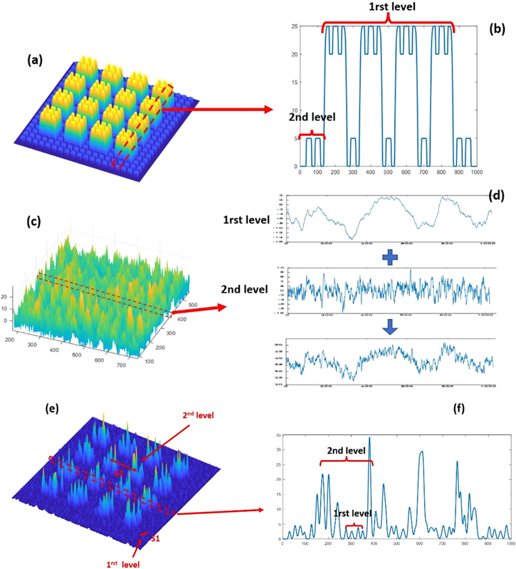
Figure 2. Examples of hierarchical surfaces exhibiting additive (deterministic (a) and stochastic (c)), and stochastic spatial hierarchy (e) along with their typical profiles (b), (d), (e) to illustrate more clearly the meaning of each hierarchy type.
Download figure:
Standard image High-resolution imageIn the context of the second approach, the different levels can be combined either additively or spatially hence we can clarify at least two terms of hierarchical surfaces: additive or spatial. In the additive hierarchy, the hierarchical surface is the sum of the heights of involved levels with weights to quantify their interaction (if any). On the other side, in the spatial hierarchy the levels are mixed spatially and the second level emerges from the aggregation of the features of the first level. Example for both cases (experimental and model) can be seen in figure 2.
3. Methodology tools
3.1. Fourier transform (FT)
The FT is an important tool for processing surface data, used to decompose a surface into its harmonic frequencies. The actual output of the transform represents the surface in the frequency domain (in other words it is the actual frequency footprint of the surface), whereas the surface data represent the spatial domain equivalent. Practically in the Fourier domain, each point can be regarded as the strength with which a certain frequency contributes to the spatial domain. The FT, being used in a wide variety of applications like image analysis, signal processing and machine learning, is an ideal candidate to be used as a tool in our case, in an effort to detect and quantify in the frequency domain the different levels of hierarchy in a multiscale surface. Since micro and nanostructured surfaces are usually measured with scanning probe microscopes (SEM, AFM), the obtained surface data are discrete having the form of a matrix z(x, y) with x = 1,...,N, y = 1,...,M and N × M the dimensions of the lattice of measurement range [14]. Therefore, one should use the discrete Fourier transform (DFT) in which the number of frequencies corresponds to the number of measurement points in the spatial domain surface.
The mathematical expression of the DFT for the discrete surface z(x, y) is given by the formula

If we assume that our surfaces are isotropic (i.e. rotationally invariant), then we can shift from 2D Fourier spectra to the 1D circularly average Fourier transform (CAFT) by changing the coordinate system from cartesian to polar and averaging over azimuthal angles.
Usually, in a typical CAFT graph (figure 3(a)), we can distinguish two regimes. The first (mid to high frequencies) there is a fixed slope in log–log axes (power law in linear axes), that points out to fractal behavior due to the power law and a flat area which points towards random behavior (white noise) at lower frequencies. The knee frequency separating these two areas defines the frequency that corresponds to the correlation length ξ of the surface. Taking advantage of these characteristics, we will show that CAFT is very helpful in both the detection and quantification of hierarchy levels.
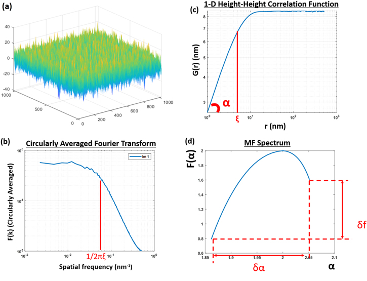
Figure 3. Example of a computer-generated scale-limited self-affine surface with rms = 6 nm, ξ = 5 nm, α = 0.7 (a) and its circularly averaged Fourier transform F(k) (b), HHCF G(r) (c) and multifractal spectrum F(α) (d). Notice the impact of ξ on F(k) and G(r) as well as the two fundamental quantities obtained from f(α) namely its horizontal spread δα and its asymmetry δ f.
Download figure:
Standard image High-resolution image3.2. Height–height correlation function (HHCF)
A common tool for quantifying correlations and detecting fundamental scales in surface data, is the ACF. ACF is the correlation of a signal (surface) with a shifted copy of itself as a function of shift distance. In other words, it is the similarity between surface heights as a function of the distance lug between them, thus revealing how the correlation between any two points on the surface changes as their separation distance changes [14, 15].
For a surface z(x, y) centralized around zero (<z(x, y)>= 0), the ACF R(m, n) can be written as:
where σ is the standard deviation of surface points, and n, m are the shifts along x and y axes respectively.
The HHCF is similar to the ACF with a minor difference that instead of summing the products of surface heights at two different points, we take the average of the square of height differences between surface points separated by a specific distance. In this case there is no need to have a well-defined mean value while the elevation rate at small distances (slope) is straightforwardly related with the fractal dimension of surface.
The mathematical formula of HHCF G(m, n) for a discrete surface data set z(x, y) defined in an area (N × M) is given by
It can be shown that HHCF is related with ACF. The relationship in 1D can be written as:

where  and σ the standard deviation of surface heights.
Looking closely at the graphical representation of HHCF (figure 3(b)) and similarly to the FT, we can see that for a random SA surface at small distances, G(r) increases following a power law r with a fixed slope ('a' which is called the roughness exponent, and is related to the fractal dimension) which points to a fractal behavior, whereas the flat part (at long distances) points to uncorrelated randomness. The knee distance separating these two regimes is actually the correlation length ξ of the surface.
As it will be shown, depending on the type of the analyzed surface and its characteristics, we may find the two methods to be more or less sensitive in detecting hierarchical levels (if present).
3.3. Multifractal analysis (MFA)
Another data analysis tool, which can be helpful when dealing with complex surfaces containing structures at different size and density, is the fractal geometry. The latter is an extremely useful method when scaling symmetries are present on a surface. In our case though and since our surfaces can be characterized by the coexistence of a variety of scales and fractal symmetries combined in complicated ways, a method to resolve such issues is the use of MFA. MFA is essentially an extension of the fractal geometry used when more than one scaling symmetries are involved. The result of MFA is a continuous parabola-like spectrum of exponents called singularity spectrum f(α) (see figure 3(d)) instead of a single fractal dimension.
In literature one can find many different methods for the implementation of MFA [11]. For surfaces and images, a commonly used implementation is the box-counting method (BCM) that measures the scaling behavior of a surface versus surface height differentiating the fractal analysis of peaks from bottom surface areas (valleys). The left branch of f(α) curve corresponds to the scaling behavior of the top segments of the surface (peaks) while the right branch indicates the scaling behavior of the bottom segments (valleys). The horizontal axis (α) handles the height segmentation of the surface for the analysis, extending from the peak region (α < 2) up to the valley region (α > 2), whereas the vertical axis f(α) reveals the fractal exponent of the segments obtained by the corresponding value of α. f(a) is always smaller or equal to 2 since the peak or valley segments of the surface cover partially the 2D plane. At the curve vertex (α = 2) the entire surface is considered and f(α = 2) = 2 subsequently. The width of the spectrum δα indicates the vertical range of surface fluctuations while the δ f = f(αmax)−f(αmin) is a common measurement of the multifractality of a surface, quantifying the asymmetry between the scaling behavior of the top (peaks) and the bottom(valleys) parts of the surface.
4. Modeling and generation of additive hierarchical surfaces
In order to build a concise methodology for the characterization of hierarchical surfaces, it is necessary to develop modeling algorithms capable to generate hierarchical surfaces of various types. To this end, first we need to produce each of their components, i.e. algorithms enabling the generation of deterministic or stochastic surfaces. Afterwards, combining the surfaces created above, we can produce surfaces exhibiting predetermined hierarchical features. The challenge here is to model the interaction between different levels to identify the essence of hierarchy in the analyzed surfaces. In this work, we will be limited to Gaussian surfaces (surfaces exhibiting a normal distribution, with skewness equal to 0 and kurtosis equal to 3), so there will be no need to describe an algorithm for generating non-gaussian surfaces with predetermined skewness and kurtosis different than 0 and 3 respectively [16]. We will also emphasize on hierarchical surfaces comprising two different kinds of stochastic surfaces, mound and SA.
Both kinds of surfaces can be generated by the same algorithm which is based on a stochastic-like inverse FT process and has been described in detail in previous works [13, 17]. For the sake of completeness, here we report it shortly.
The first step of the algorithm is to define the input ACF R(m, n) in analytical or numerical form. The kind of the generated surface is determined by the form of the ACF. For fractal SA surfaces, a usual choice is the following formula:

where ξ x and ξ y are the correlation lengths along the axes x and y respectively and α the roughness exponent of surface which is linked to the fractal dimension dF since dF = 3−α. In the case of isotropic surfaces ξ x = ξ y = ξ.
On the other side, when the aim is the generation of mounded surfaces, the input ACF reads:
where λ is the average mound separation length and J0 is the zeroth-order Bessel function
Three parameters are used to describe the surface besides standard deviation σ: the system correlation length ζ, the roughness exponent α, and the average mound separation λ. The lateral correlation length ξ defined by R(ξ) = 1/e is a function of both ζ and λ in mound surfaces. For example, when ζ = λ then ξ = 0.27λ. [13]
In both cases of ACF, the next step is to take advantage of the Wiener–Khinchine theorem according to which the FT of the ACF R(m, n) equals the power spectrum of the surface to be generated.
In order to randomize the phases of the FT, a white noise is generated and after normalization, its FT is obtained in order to be multiplied with the square root of the power spectrum obtained by the ACF. In the final step, we take the inverse FT of the above FT product and this outputs our Gaussian rough surface. By tampering with the ACF (using formulae (5) or (6)), we are able to produce different kind of surfaces such as mounded or SA surfaces.
The generated surfaces can be then combined properly either linearly or nonlinearly in order to produce a surface that exhibits hierarchical features. To achieve this, the spatial scales of added surfaces, defined by the correlation length ξ and mound separation λ in SA and mound surfaces respectively, should differ significantly, so that hierarchy is emerged in the final comprised surface. We may also have different combinations of SA and mounded surfaces, to accommodate the two levels of the synthesized hierarchical surfaces as shown in figure 4.
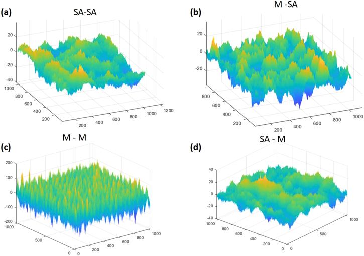
Figure 4. Examples of additive hierarchical surfaces with different combinations of levels: (a) self-affine and self-affine (SA–SA), (b) mounded and self-affine (M–SA), (c) mounded and mounded (M–M) and (d) self-affine and mounded (SA–M).
Download figure:
Standard image High-resolution imageIn all cases of additive hierarchy consisting of two levels, the obtained hierarchical surface zh (x, y) may be calculated using the following formula

where z1 and z2 are the two components comprising the first (large scale) and the second (fine scale) levels respectively. The multiplicative factor α defines the linear or nonlinear character of hierarchy composition and can be used for the quantification of the interaction between hierarchy levels. When b = 1 the levels are superimposed linearly with no interaction and information exchange between them. This type of hierarchy can simulate the cases where the two processes contributing to surface roughening act independently each other. On the other side, when b is a function of z1 then the addition of the second level is affected by the local values of the first level z1, i.e. the second mechanism responsible for roughness creation takes into account the pre-existent surface morphology of the first level, shaping accordingly the final output of hierarchical surface.
Here, in order to provide a continuous transition from the linear (non-interactive) to nonlinear (interactive) case, we set b(z1) = 1−c + c*z1. For c = 0 the multiplicative factor b = 1 and we are in the realm of linear hierarchy whereas for c = 1 then b = z1 and the addition of the second level depends strongly on the first level leading to nonlinear hierarchical surfaces (see figure 5). Therefore, c controls the amount of nonlinear combination of hierarchy levels and therefore the degree of their interaction and information flow from the first to the second one. Figure 6 illustrates a series of hierarchical surfaces in both top–down and 3D views with increased nonlinearity tuned by the value of c which changes from 0 to 1. One can clearly notice the impact of c increase on the final hierarchical surface we obtain. In order to make clear the presence of interaction, we also use the term of i-hierarchy when level interactions take place. In the case of i-hierarchy we can for example condition the addition of the second level. to depend upon the height of the first level.
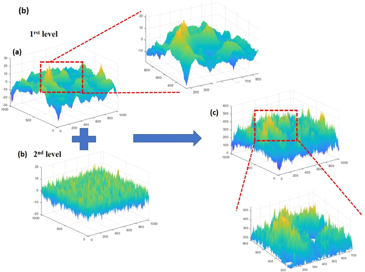
Figure 5. Example of i-hierarchy for c = 1, where two levels (a) and (b) are added to form a hierarchical surface (c). It is visible that interactions are more intense in the vicinity of the peaks of the first level.
Download figure:
Standard image High-resolution image
Figure 6. Examples of i-hierarchy (both surface 3D and image 2D representation) where we condition the addition of the second level depending upon the heigh of the first level (a) SA–SA SA (1rst level rms = 6 nm, ξ = 100 nm, α0.8 and 2nd level: rms = 3 nm, ξ = 5 nm and α0.5) and (b) mound–SA (1rst level rms = 6 nm, ξ = 200 nm, α0.8, λ = 50 nm and 2nd level: rms = 3 nm, ξ = 50 nm and α0.5).
Download figure:
Standard image High-resolution imageIn other words, the amplitude of fluctuations of the resulting surface will be larger near the vicinity of the peaks of the first level whereas smoother near the vicinity of the valleys of the first level (see figure 5).
The intensity of this interaction between the two levels (a) and (b) is controlled from the value of c and so the larger the value of c the stronger the intensity of interaction (see figure 6)
Another case of i-hierarchy could be when the second hierarchy level may depend on other higher-order local morphological characteristics of the first level (in different words the existence of the second level may be topographically selective). In equation (7) for example, the parameter c could change in respect to the first or second derivative of the 1st level, getting maximum values at areas with large slopes or curvatures respectively. The later actually meets application in experimental cases, as for example, one may require to enhance local roughness by applying a second mechanism of roughening selectively only on certain 'active' parts of the 1st level surface, while leaving almost intact the rest of it.
5. Quantification through fourier and correlation analysis: the case of stochastic additive hierarchy
Besides definitions, classification and modeling, what is of equal importance is the quantitative characterization of hierarchical surfaces, a critical and not easy endeavor that also concerns the applications in real experimental surfaces. We will try the conventional methods of correlation and Fourier analyzes to justify their pros and cons in the identification and characterization of different types of hierarchical surfaces. Also, we will use the MFA to detect and quantify the amount of interaction between different surface levels.
5.1. Non-interactive additive hierarchy
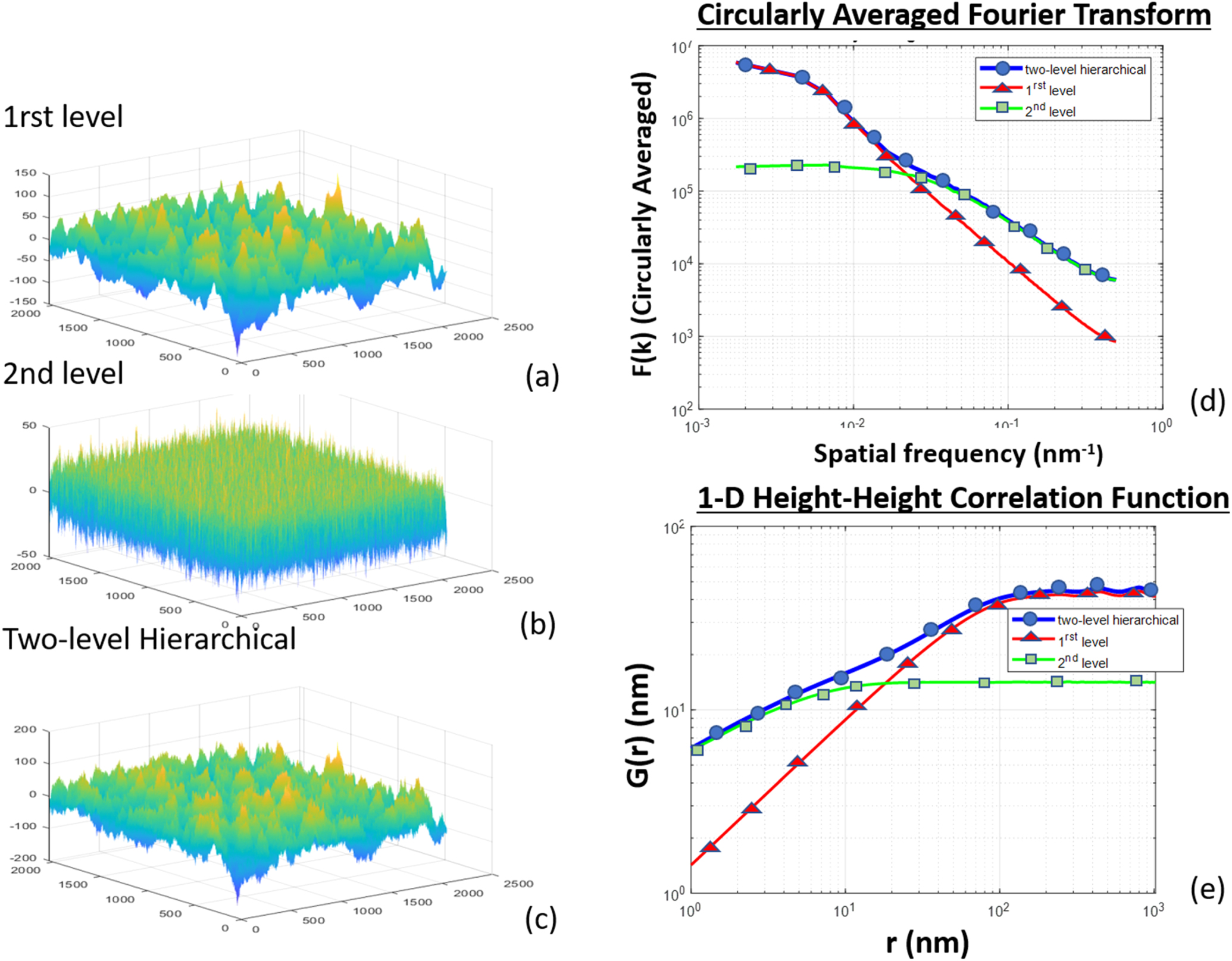
Figures 7 and 8 show the cases of the combination of either two mound (figure 7) or two SA (figure 9) surfaces. Figures 7(a) and (b) display examples of surface morphologies of the first (large λ) and second level (small λ) along with the hierarchical surface formatted by their linear addition. The existence of the two different mound levels can be easily spotted from the CAFT of the hierarchical surface (blue line in the diagram of figure 7(d)) by the two peaks which depict the approximate periodicity of the two levels in our hierarchical surface. The presence of the two mound levels is also observed in the HHCF of the hierarchical surface (blue line in figure 7(e)) with the superimposed oscillations in the short and large distances respectively. In the second case (SA–SA), the SA morphologies of the two added levels and the final hierarchical surface are illustrated in figure 8(c). In the example we show, the first level has larger correlation length (ξ1 > ξ2) and is characterized by bolder peaks and valleys. The presence of the two different SA levels can be spotted by the presence of the two knees in both the Fourier spectrum and the HHCF graph of the hierarchical surface as shown in figures 8(d) and (e) respectively.
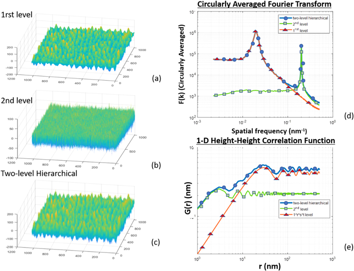
Figure 7. FT and HHCF of mound–mound example case (1rst level: rms 30 nm, ξ 200 nm, alpha 0.8, λ 50 nm and 2nd level: rms 15 nm, ξ 200 nm, α 0.8, λ 5 nm), where the two mound levels can be easily spotted by the double FT peaks or the low and high distance HHCF fluctuations.
Download figure:
Standard image High-resolution image
Figure 8. FT and HHCF of SA–SA case (1rst level: rms 30 nm, ξ 70 nm, α = 0.8, and 2nd level: rms 10 nm, ξ 5 nm, α 0.5), where the presence of the two SA levels is observed from the 2 knees in both HHCF and FT spectrum.
Download figure:
Standard image High-resolution image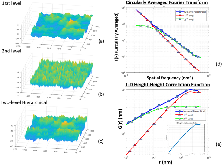
Figure 9. FT and HHCF of SA–SA with no knee (a2 = 0.4) (1rst level: rms 6 nm, ξ 100 nm, α 0.7 and 2nd level: rms 3 nm, ξ 10 nm, α 0.4), where is it unclear whether we are dealing with a hierarchical surface or a SA surface.
Download figure:
Standard image High-resolution imageIn the case of the combination of SA levels though there are cases for which the analysis of the CAFT and HHCF diagrams of the hierarchical surface is not clear enough and may lead to a misconception. This is shown in figure 9, where the Fourier spectrum of the resulting hierarchical surface does not exhibit a knee that would have depicted the presence of two different levels. On the contrary, a power law is observed throughout the entire frequency spectrum which points to a single SA surface. Similarly, the HHCF of the total hierarchical surface shows a power law increase till a saturation at large distance after a single knee pointing out again a single SA surface. This result occurs whenever the roughness exponent of the second level with the smaller ξ is set close to 0.4, independently of the specific values of ξ1 and ξ2 and undermines the straightforward detection of hierarchy from either the Fourier spectra or the HHCF graph. Nevertheless, a closer inspection of HHCF curve can reveal an indirect evidence for the existence of hierarchy, especially when we compare it with the HHCF of a SA surface with roughness exponent equal to 0.4 (see inset in figure 9(e)). Both the minor change in the slope of the HHCF graph (mid to high distances) and also the steeper knee at the high distances before saturation can be used to differentiate the HHCF of the hierarchical surface from the HHCF of the single SA surface where the knee is much smoother and the slope more uniform.
The final cases contain the mixed hierarchical combinations of mound with SA morphologies. Figure 10 shows an example when the mound level is the first and SA the second level (λ1 = ξ2), while figure 11 displays the complementary case with the mound surface being the second level added to a SA surface (ξ1 > λ2). Similarly, to the case of two mound levels, here as well, we may spot the presence of the mound level from the prominent peak in the Fourier spectra (see figures 10(d) and 11(d)) or the oscillations in the HHCF graphs (see figures 10(e) and 11(e)). At the same time, the raised low frequency part of the Fourier spectra depicts the presence of a SA coexisting level. In terms of HHCF, the raised short distance part in the case of mound–SA hierarchy and the knee in the SA–mound hierarchy signify the presence of the SA level. However, in accordance with the above discussion about the hidden SA–SA hierarchy, a simple inspection of the HHCF of a SA–mound hierarchical surface may also lead to confusion. The raised short distance part may be negligible and the HHCF can be considered to characterize a single mound surface. A parallel examination of the FT is valuable in this case since it can easily disclose the hierarchical nature of the analyzed surface by the identification of the presence of both a well-defined peak and a continuously decreasing FT on both sides of the peak.

Figure 10. FT and HHCF of mound–SA case (1rst level: rms 30 m, ξ 200 nm, α 0.8, λ 50 nm and 2nd level: rms 15 nm, ξ 50 nm, α 0.5), where the presence of the mound level can be spotted in both FT (peak) and in the HHCF's high distance fluctuations and the presence of the SA level is noticeable in the sloped and raised low frequency part of the FT.
Download figure:
Standard image High-resolution image
Figure 11. FT and HHCF of SA–mound case (1rst level: rms 6 nm, ξ 100 nm, α 0.7, λ 50 nm and 2nd level: rms 3 nm, ξ 10 nm, α 0.5, λ 10 nm), where again the presence of the mound level can be spotted in both FT (peak) and in the HHCF's low distance fluctuations and the presence of the SA level is noticeable in the sloped and raised low frequency part of the FT.
Download figure:
Standard image High-resolution imageThe marginal ones (where hierarchy is not easily distinguishable), is that no a metric (HHCF or FT) on its own is powerful enough to be individually used, in order to identify and quantify hierarchy. At least not in all cases. It is though observed, that both methods may exhibit an unsteady (high or low depending upon hierarchy composition and surface parameters), unrelated to each other and unconditional sensitivity on different types of hierarchy and different types of hierarchical characteristics. Taking this into account, both methods should be investigated each time, as either one of them could be sufficient, or a hybrid application of them should be taken under consideration, by which both of them, working in parallel will be able to provide us with the necessary information on each case. For example, in the case of a mound hierarchical level, the FT works better in detecting levels by recognizing the spectrum peak/peaks. HHCF on the other hand provides aid in the recognition of SA levels when FT is weak on detecting them, as in some cases HHCF exhibits higher sensitivity over FT.
5.2. Interactive additive hierarchical surfaces
For the case of i-hierarchy, in figure 12 we can see FT and HHCF examples for different hierarchy compositions (SA–SA, mound–SA and SA–mound) for varying values of the nonlinear parameter c.

Download figure:
Standard image High-resolution image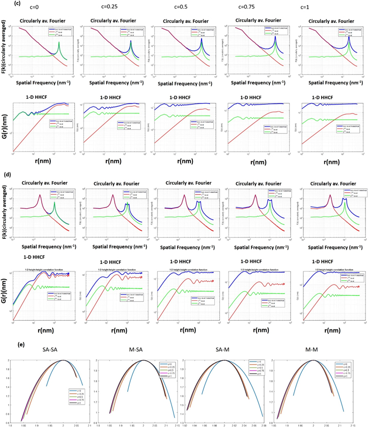
Figure 12. FT and HHCF of two level (a) SA–SA hierarchical surface (1rst level: rms = 6 nm, ξ = 100 nm, α = 0.8 and 2nd level: rms = 3 nm, ξ = 5 nm, α = 0.5) (b) M–SA hierarchical surface (1rst level: rms = 6 nm, ξ = 200 nm, α = 0.8, λ = 50 nm and 2nd level: rms = 3 nm, ξ = 50 nm, α = 0.5), (c) SA–M hierarchical surface (1rst level: rms = 6 nm, ξ = 100 nm, α = 0.8, and 2nd level: rms = 3 nm, ξ = 50 nm, α = 0.5, λ = 5 nm) and (d) M–M hierarchical surface (1rst level: rms = 6 nm, ξ = 200 nm, α = 0.8, λ = 50 and 2nd level: rms = 3 nm, ξ = 100 nm, α = 0.5, λ = 10 nm) (e) multifractal analysis of all level combinations where we can see that hierarchy is distinguishable by both HHCF and FT while i-hierarchy is noticed in the multifractal analysis.
Download figure:
Standard image High-resolution imageIn the case of SA–SA composition (figure 12(a)) we can see that as c increases the knee area becomes less intense and hierarchy can still be identified though a little bit harder, especially if HHCF is only taken under consideration.
In the case of mound–SA hierarchy (figure 12(b)), as c increases, the periodicity of the first (mound) level becomes a little bit vague (peak of the mound level becomes less prominent) as the second SA level tends to break the periodicity of the mound level. Yet hierarchy can still be recognized in both FT and HHCF as both, the peak in FT and fluctuations at large distances in HHCF are still detectable.
In the case of SA–mound surfaces (figure 12(c)), the FT form stays merely unaffected and one detects the mixed hierarchy as the peak though slightly faded can be still recognized, whereas in the HHCF case the presence of an SA level slightly disappears as the second level dominates and the slope of the HHCF tends to disappear.
In the case of mound–mound (d), as c increases, the periodicity (peak) of the first level fades a little bit whereas the periodicity of the first level remains the same. This behavior can be also verified in the HHCF as the fluctuations are a little bit less intense, though still visible.
As we can see, once more for i-hierarchy this time, in order for us to detect hierarchy, a hybrid use of FT and HHCF is preferred, as each one of the methods, if applied alone, may lead to misconception/wrong assessment. For detecting i-hierarchy though, that is when linearity is broken (c > 0), if one relies only on FT and HHCF (figures 12(a)–(d) there is no way to tell whether we have simple linear hierarchy or nonlinear i-hierarchy. That is why we deploy at this point a MFA, which is based in the calculation of the MF spectrum, as shown in figure 12(e) for all cases of different level combinations. As we can see when c becomes larger than zero and linearity breaks, MF spectrum will either lose its symmetry, or change symmetry drastically, because by increasing interactions near the peaks of the first level, we are essentially increasing the contribution of scaling content of peaks in the mf spectrum (left side of the mf spectrum). That is why in the case of SA–SA the symmetry breaks and in the three other cases (M–SA, SA_M and M–M), the symmetry changes from being in favor of the valleys, towards favoring the peak side.
This behavior can be also observed in the graphical representation of Kurtosis versus c. More specifically in figure 13(b) the mentioned symmetry changes in SA–M, M–SA and M–M cases, when c becomes larger than 0, as skewness changes sign. In figures 13(c) and (d) also we observe that, as c increases, both df and da increase, indicating the expansion of the inhomogeneity between the scaling behavior of the top (peaks) and the bottom(valleys), in favor of the peaks and at the same time the increase of the range of surface fluctuations. The increase of da can be also linked to the increasing kurtosis. We can also observe that SA–M and M–M cases have limited effect on da whereas df is sensitive in all cases and distinguishes the effect of nonlinearity. Generally, when a M level is involved the change of sign of df (bocoming positive) points towards nonlinear interaction and when only SA levels are involved when df becomes larger than 0 we again have evidence of nonlinear interaction. Generally, for all combinations we may use both df and skewness for the detection of nonlinear interactions between hierarchical levels and marginally also use them for the quantification of the level of interactions (as that level is controlled by c).

Figure 13. Diagrams illustrating the dependence on parameter c of (a) multifractality asymmetry δ f and (b) spectrum width δα (c) skewness, (d) kurtosis, for all level combinations, depicting the symmetry change as c increases.
Download figure:
Standard image High-resolution image
The results can be summarized in the following table 1, by which we can conclude that in order to detect hierarchy and identify the type of involved levels, we may use a hybrid combination of Fourier and HHCF analysis. FT and HHCF can be also used for the quantification of hierarchy, whereas for the detection of nonlinear interactions between the hierarchical levels (interactive hierarchy), a MFA is required.
Table 1. Summarized results of the applicability of each analysis method.
| FT | HHCF | MFA | |
|---|---|---|---|
| Detection of hierarchy | x | x | |
| Identification of level type | x | x | |
| Quantification of hierarchy | x | x | |
| Detection of nonlinear interactions | x |
6. Conclusions
Hierarchical morphologies are important because they enrich surfaces with novel properties and enable multifunctionality. A variety of different fabrication techniques can be deployed to produce such surfaces while their enhanced properties can be exploited in numerous applications. In order to be able to control the hierarchical morphology of the produced surfaces though we need to be able to characterize and quantify the type and amount of hierarchy.
Towards this goal, in this paper an effort has been made to use Fourier, correlation and MFA, which showed promising results in detecting and quantifying the levels that consist the final hierarchical surface. They also show good results in obtaining roughness parameters of the different levels with some limitation especially when high frequencies dominate the smaller level. More specifically, in the direction of additive hierarchy, we are able to detect and quantify the different levels of hierarchy by identifying either the knees in FT and HHCF or the peaks and fluctuations in FT and HHCF respectively. Finally, even though for the detection of hierarchy, the hybrid use of FT and HHCF is enough, when dealing with i-hierarchy where hierarchy levels are combined nonlinearly, after the detection of hierarchy and in order to pinpoint the existence of i-hierarchy, we need to use a MF and/or higher moment analysis which reveal and quantify the presence of interactions between the different levels of hierarchy.
Data availability statement
All data that support the findings of this study are included within the article (and any supplementary files).