
Abstract
SPPARKS is an open-source parallel simulation code for developing and running various kinds of on-lattice Monte Carlo models at the atomic or meso scales. It can be used to study the properties of solid-state materials as well as model their dynamic evolution during processing. The modular nature of the code allows new models and diagnostic computations to be added without modification to its core functionality, including its parallel algorithms. A variety of models for microstructural evolution (grain growth), solid-state diffusion, thin film deposition, and additive manufacturing (AM) processes are included in the code. SPPARKS can also be used to implement grid-based algorithms such as phase field or cellular automata models, to run either in tandem with a Monte Carlo method or independently. For very large systems such as AM applications, the Stitch I/O library is included, which enables only a small portion of a huge system to be resident in memory. In this paper we describe SPPARKS and its parallel algorithms and performance, explain how new Monte Carlo models can be added, and highlight a variety of applications which have been developed within the code.
Export citation and abstract BibTeX RIS

Original content from this work may be used under the terms of the Creative Commons Attribution 4.0 license. Any further distribution of this work must maintain attribution to the author(s) and the title of the work, journal citation and DOI.
1. Introduction
Materials inherently interact with their environment at the atomic scale, e.g. via mechanical, chemical, or electrical processes. However, their response is often manifested and observed at the meso or continuum scales. Monte Carlo (MC) models are powerful computational tools for helping bridge these length and time scales. Three important variants for materials modeling are kinetic Monte Carlo (KMC), rejection KMC (rKMC), and Metropolis Monte Carlo (MMC) methods.
In KMC and rKMC models, important events such as diffusive hops or reactions are defined along with their rates to capture the relevant physical underpinnings of the model. These definitions can reflect both internal interactions between atoms or mesoscopic particles as well as external fields such as an electric potential, temperature gradient, or background concentration profile. Efficient algorithms can select events one after another with the correct relative probabilities and update the state of the system in a time-accurate manner, without the need to follow detailed atomic motion or spend CPU time waiting for interesting events to occur.
For KMC this procedure requires knowing the rates of all events that may occur next. In the rKMC variant, pre-computation of some or all of the rates can be avoided if events can be partitioned into natural subsets (e.g. per lattice site or per particle), and a so-called null event defined for each subset. A site or particle can then be chosen randomly and only rates for events involving that site or particle need calculation to determine the next event, which may turn out to be null (i.e. no diffusive hop or reaction).
By contrast, MMC models are not time-accurate but can be used to sample the states of an equilibrated system (e.g. [1–4] for molecular modeling) or to dynamically evolve a system toward an equilibrated state (which may never be reached). In this paper our focus is on the latter. A candidate event is picked, the energy change it induces in the system is calculated, and the event is accepted or rejected based on a Metropolis criterion which is a function of temperature. MMC models also allow unphysical events to be defined, such as swapping the atomic species of two atoms, in order to computationally accelerate the time evolution of the system.
In a materials modeling context both on-lattice and off-lattice models of all three variants—KMC, rKMC, MMC—are widely used; see examples in reviews by Chatterjee and Vlachos [5] and Voter [6], as well as articles cited later in this paper. On-lattice models are the primary focus of this paper; they represent a material on a regular grid, with one or more variables defined at each grid point. By contrast, off-lattice models represent a material as a collection of particles at arbitrary locations, typically as either atoms or mesoscale entities. Generally, on-lattice models are simpler and more computationally efficient, while off-lattice models can more accurately represent a wider range of material behavior, especially at the atomic scale.
Exact KMC and rKMC algorithms are fundamentally serial, because selection of the next event may depend on the state of the entire system after the previous event. By contrast, MMC algorithms can often be easily parallelized by performing multiple events simultaneously so long as it is done in a manner which satisfies detailed balance (discussed further in the next section). In practice, this generally means two events can be performed simultaneously if their spatial separation is large enough that the outcome of one event does not influence the outcome probabilities of the other event. Thus models whose energy computations are local (involving only a site and its near neighbors) are amenable to parallel execution.
The same idea to perform spatially local events simultaneously can be exploited to parallelize KMC and rKMC models. The simulation domain is partitioned across processors and each processor performs events only within its subdomain. This can result in algorithms that are no longer exact, but which are still sufficiently accurate for practical modeling purposes.
One such category of parallel algorithms are asynchronous in that time does not advance uniformly across all subdomains. This may require a different methodology for choosing events at subdomain boundaries [7, 8] or periodically synchronizing and 'rewinding' in time to resolve conflicting events which occurred at the boundaries [9–11]. Asynchronous algorithms are challenging to parallelize efficiently, especially at large scale.
By contrast, synchronous algorithms offer a simpler route to parallelization. A notable example is the synchronous sub-lattice (SSL) algorithm of Shim and Amar [12]. Each processor performs events within a subset of its subdomain with no possibility of conflict with events performed by other processors. This is because the subsets are defined so that their boundaries are not updated at the same time by neighboring processors. This introduces errors relative to exact serial KMC, but as discussed in sections 2.7 and 2.9, the errors can be estimated and bounded.
Examples of parallel on-lattice KMC modeling based on the SSL algorithm include billion-site Ising models [13], thin film growth [14], charge carrier transport in organic semiconductors [15], vacancy diffusion in iron [16], and solute interactions with point defects in metal alloys [17]. To our knowledge the codes used for these papers are not publicly available. Two open-source software packages for KMC-based materials modeling are the kmcos framework (formerly kmos) [18, 19] and KMClib library [20, 21]; they also enable users to implement their own models. However kmcos does not operate in parallel, and the focus of KMClib is not on the style or scale of parallelization which the SSL algorithm enables.
In this paper we describe the open-source parallel SPPARKS kinetic Monte Carlo simulation code [22]. It was initially made publicly available for download in 2009; we recently moved its development to GitHub [23]. The code primarily supports on-lattice MC models, though it also has modest support for simple off-lattice MMC models as described in section 2.13.
SPPARKS has two notable features which we detail. The first is efficient spatial parallelization of on-lattice KMC, rKMC, or MMC models. For KMC and rKMC, it implements the approximate SSL algorithm [12]. The code has a heuristically adjustable setting which allows the user to trade-off parallel efficiency against accuracy in a manner that enables accurate simulations. For MMC, it provides options for more fine-grained parallelism. The second feature is modular design, making it relatively easy for users to extend SPPARKS with code for a new on-lattice MC model or application, and thus enable large-scale parallel simulations with their model.
The remainder of the paper is organized as follows. Section 2 describes the algorithms used by SPPARKS to achieve parallelism, including partitioning of the simulation domain across processors, communication between processors, and various methods to allow multiple MC events to be performed simultaneously. In section 3 we describe how the code is designed to be extensible so that users can add new models which leverage the algorithms of section 2. In section 4, benchmark timings are presented which illustrate the code can efficiently and scalably perform simulations on large parallel machines. Then in section 5 we highlight the variety of on-lattice material modeling applications which the authors and their collaborators have implemented within SPPARKS over the last decade. Finally, in section 6 we comment on new capabilities which could potentially be added to the code.
2. Algorithms
SPPARKS consists essentially of two parts: a suite of applications which implement specific models, and a core functionality used by all the applications. This section describes that functionality and the serial and parallel algorithms it uses. The next section 3 will explain how new applications are implemented using this framework.
2.1. Lattices
In the context of on-lattice Monte Carlo (MC) methods for materials modeling, a lattice is simply a graph with vertices and edges. Each vertex is a lattice site at a spatial location, which has some number of nearby neighbor sites, enumerated by graph edges. As illustrated in figure 1 lattices in SPPARKS can be 1d, 2d, or 3d, and may be regular or irregular.

Figure 1. Diagrams and images of lattices supported by SPPARKS. For 1d systems: (a) line and (b) random. For 2d systems: (c) square4, (d) square8, (e) triangular, and (f) random. For 3d systems: (g) cubic6 and (h) custom. Additional 3d lattices and (h) are described further in the text. Edges are drawn to indicate which vertices are neighbors of each other (except in 3d). The large red sites are the neighbors of a single large black site. Note: In the print version of this paper no figures are in color. Please see the open-access on-line version of the paper for color versions of all the figures.
Download figure:
Standard image High-resolution imageA regular lattice has sites at uniformly spaced points, and the same number of neighbors for each site. Note that a site's neighbors need not be defined as simply the set of its nearest neighbors; for the square8 lattice in figure 1(d), the MC neighbors are the eight first- and second-nearest neighbors surrounding each site. An irregular lattice can position its sites anywhere, and define different numbers of neighbors per site. For the two random lattice sub-figures (b) and (f), the set of neighbors for each site is defined by a cutoff distance rcut .
The regular 3d lattice (g) in the figure is for a simple cubic lattice where each site has 6 neighbors, its nearest neighbors in each dimension. There is also a cubic26 lattice where each site has 26 neighbors, namely its first-, second-, and third-nearest neighbors. SPPARKS also supports 3d body-centered cubic (bcc) and face-centered cubic (fcc) lattices, common in solid-state physics, with 8 and 12 neighbors/site respectively. There is also a fcc/octa/tetra lattice which adds octahedral and tetrahedral interstitial sites to the fcc lattice; it was added to support a specific application described in section 5.5.
A regular lattice may be periodic or non-periodic in any dimension with respect to the simulation box. Lattice sites on a periodic face have neighbor sites on the opposite face; sites on a non-periodic face do not, which is a method for modeling a free surface, e.g. for thin film growth.
Custom lattices in one, two, or three dimensions are also supported where the site coordinates and their neighbor connectivity are enumerated in an input file. Sub-figure (h) is a fine-grained custom 3d lattice with 35 000 sites (not visible) which triangulate the surface of a pill-shaped biological cell. Each site has (on average) 6 neighbors. The figure shows a snapshot of a simulation with a 3-state Ising model (red,yellow,purple) which was used to simulate the effect of antimicrobial peptides (AMPs) on cell membrane permeability. Its implementation in SPPARKS and the meaning of the figure are discussed further in section 3.
Each application in SPPARKS defines what data it stores at each lattice site. This can be any number of integer or floating point values. These values can be used and/or updated by the application in its MC calculations, initialized by input script commands, or input/output from/to files. As explained in section 2.8, in a parallel simulation each processor also communicates its per-site values to other processors.
As explained in the next subsection, once the dimensionality of the physical system is defined, it often does not matter which lattice is used to calculate the Hamiltonian that underlies the Monte Carlo model, though it may affect its parameters. The equation is typically a simple function of individual lattice sites and their neighbors. In practice, if the sites represent atoms, a solid-state lattice corresponding to the crystalline solid-state material is convenient. For mesoscale models a simple square or cubic lattice may be used, since each lattice site represents a coarse-grained chunk of physical material.
2.2. On-lattice Monte Carlo
On-lattice MC models define the system energy as a sum (over lattice sites) of per-site energies. The energy at each site is a function of the site value(s) and its neighboring site values.
As examples, consider the standard Potts model [24–26], where each lattice site has an integer spin value Si
from 1 to a user-defined value Q. Q = 2 is a canonical Ising model. Also consider a single-species diffusion model where a site is either occupied with  or unoccupied (vacancy) with
  . Both models define a single integer value at each site.
The Hamiltonians for the energy of a site i in these models with M neighbors (as defined by the lattice), can be written as follows, for two variants of the diffusion model:


In each case the energy of the entire system is simply Hi
summed over N sites. For the Potts model,  is 0 if
  and 1 if
  . For both diffusion models, a vacant site with
  has
has  , regardless of its Sj
neighbor values. For an occupied site with
, regardless of its Sj
neighbor values. For an occupied site with  ,
,  , so that
  is effectively the coordination number of the site.
For the linear diffusion model, the site energy is a linear function of coordination number. For the nonlinear model, the coordination number is the argument to a function  which returns an energy. In SPPARKS the user can input a list of function return values. If desired, they can be pre-calculated using a classical molecular dynamics code with a suitable empirical interatomic potential or via density functional theory (DFT) quantum calculations so that the MC model represents a real material. See section 5.5 for an example of the latter.
An on-lattice MC model also defines 'events' that can take place at each site to change the value(s) of the site and also potentially the values of one or more of its neighbor sites. For Potts models an event changes the spin of a single site, which is termed Glauber dynamics. In general, a site can perform any of Q − 1 possible events to flip to a different spin value. Or, as discussed in section 5.1, an application using the Potts model may choose to limit possible flips to site values that match a neighboring site.
For diffusion models, events are typically defined by Kawasaki dynamics where two neighboring sites exchange their values. Such swaps are 'conservative'; if site values represent different materials or material phases, the amount of each material or phase is the same before and after the event. When vacancies are present, events need only be defined for occupied sites. Each occupied site can potentially perform one of multiple events, i.e. an exchange with any of its unoccupied neighbor sites.
SPPARKS can run these kinds of on-lattice MC models in one of three modes: kinetic MC, rejection kinetic MC, and Metropolis MC. As explained in section 3, a developer of an MC application can choose which mode(s) it will support by implementing the appropriate methods.
2.3. Kinetic Monte Carlo
The first mode is kinetic Monte Carlo (KMC in this paper) [6], also sometimes called rejection-free KMC or non-equilibrium MC. (The latter term is also used for rejection KMC, discussed next.) Each site defines zero or more events it can perform and an associated kinetic rate (or propensity) for each event. These propensities are typically not only related to energy changes in the Hamiltonian when an event takes place, but also to the temperature-dependent probability of crossing an energy barrier. The standard KMC algorithm for picking the next event with correct statistical probability relative to all other possible events, and also computing the time at which it occurs, is outlined in figure 2.

Figure 2. Kinetic MC algorithm to pick the next event m and calculate its associated time increment  in a statistically consistent manner. There are N possible events to choose from, each with propensity (or rate) pi
. The total propensity
in a statistically consistent manner. There are N possible events to choose from, each with propensity (or rate) pi
. The total propensity  is the sum of all N propensities.
Download figure:
Standard image High-resolution imageInterestingly, this algorithm has been independently formulated at least three times in different contexts. First by Bird [27, 28], for his particle-based Direct Simulation Monte Carlo method used to simulate rarefied gas flow, as an algorithm for updating time after gas particle collision events. Second by Bortz et al [29], for their BKL or N-fold way algorithm to efficiently evolve the Ising model in statistical physics simulations. And third by Gillespie [30, 31], as part of his Stochastic Simulation Algorithm (SSA) for time evolution of a biochemical reaction network of coupled ODEs within a well-mixed small volume (e.g. a biological cell) containing multiple molecular species at different concentrations.
In the SPPARKS context, the KMC algorithm is used to choose a single site (from a collection of N sites) to perform the next event, with the correct relative probability. If the selected site defines more than one possible event, the application uses an additional procedure to select one of them.
SPPARKS implements three solvers for the KMC algorithm, all of which are described in [32]. Their computational cost to choose the next site from N sites is O(N),  , and O(1) respectively. Internally, they store the current total propensity for each site in a data structure that enables them to implement step (4) of figure 2 in different ways: by scanning a list of N propensities (O(N) effort), by walking a binary tree with the N propensities at its leaves (
 effort), or via a more complex composition/rejection data structure and methodology (O(1) effort) described in detail in [32].
Once an event is selected, the MC application performs the event, which typically changes the site value(s) and possibly the values of one or more nearby sites. The new state of the system changes what events are now possible for both the selected and nearby sites as well as their propensities. The altered site propensities are calculated and passed to the solver, which updates its internal data structure and the total propensity  of figure 2. The updates must also be done with O(N),
  , or O(1) cost to maintain the solver's scalability.
2.4. Rejection kinetic Monte Carlo
The second mode is rejection KMC (rKMC in this paper), also called null-event MC or non-equilibrium MC [5]. As with KMC, each site defines a set of events it can perform with associated propensities that sum to the site propensity pi
. In this case, pi
must have a well-defined upper bound pmax
. Conceptually, the propensity of each site is then set to pmax
by adding a null event with propensity  . The event is 'null' because if it is selected, no event is performed.
The advantage of rKMC over KMC is simplicity, particularly when implementing an MC application. No list of competing propensities for all sites need be maintained and thus no KMC solver is required to select the next event. Instead, a site is chosen randomly, and a second random number is used to select an event for that site, which may be the null event. The system clock can be updated the same as for KMC, whether the event is null or not. However, since the summed propensity  in figure 2 is constant due to the null events, the clock can instead be updated more coarsely after a large number of events (null or otherwise) have occurred. Once an event is performed, there is no need to update the propensities of any of the affected sites. That calculation only need be performed once a site is selected and enumerates its events.
The disadvantage of rKMC is that the aggregate propensity of the null events across all sites may be large, and thus there can be a high probability of no event occurring at most iterations of the rKMC algorithm, decreasing its efficiency. In particular, if there are only a handful of large propensity (high rate) sites in the model, the null-event propensity will be large for all other sites, resulting in a high probability of selecting a null event. The trade-off between these effects and thus the relative computational speed of the rKMC versus KMC modes is strongly model-dependent.
Importantly, both the KMC and rKMC algorithms track the dynamic evolution of the system in a time-accurate manner. If the application defines event propensities (rates) that are physically accurate, then the KMC algorithm of figure 2 calculates a statistically exact time increment for each event's occurrence, and the resulting SPPARKS simulation is also time-accurate.
2.5. Metropolis Monte Carlo
The third mode is Metropolis Monte Carlo (MMC in this paper), also called barrier-free MC. As with rKMC, a site is chosen randomly for the next possible event. No propensities or rates need be assigned to events; if multiple events can occur at a selected site, each can be selected with equal probability. The energy change the selected event induces in the system (all affected sites) is computed using the Hamiltonian defined by the model, and the event is accepted or rejected with the following probability P (Metropolis criterion):

where  , kb
is the Boltzmann constant, and T is the temperature of the simulated system (set by the user). If
, kb
is the Boltzmann constant, and T is the temperature of the simulated system (set by the user). If  , the event decreases system energy and is always accepted. If
  , the event increases system energy and is accepted with a fractional probability which rapidly shrinks as the size of
  grows. Increasing T makes it more likely for energy-increasing events to be accepted.
MMC offers much greater great flexibility in defining events, since there is no requirement to compute event propensities. As explained in section 2.7, sites can be looped over in a variety of ways (not just random selection) to speed up a simulation or enable parallelism. Unphysical events, such as swapping the chemical identities of two adjacent atoms or particle deletion/creation/mutation, can be defined and performed. In general, the relative frequencies for selecting different events can be altered at will, so long as the constraint of 'detailed balance' is observed, meaning that (a) for any event that occurs, the reverse event can also occur and (b) the relative probability of selecting a forward versus reverse event equals the relative probabilities of the final and initial states at thermal equilibrium.
A disadvantage of MMC is that there is no inherent physical time associated with an event, since rates enable that calculation in KMC and rKMC models. Instead the Metropolis algorithm evolves the system from the initial state towards a stationary distribution of states, corresponding to thermodynamic equilibrium at temperature T. Often this distribution of states will be clustered around a local or global potential energy minimum, e.g. a Boltzmann-weighted distribution of energies. However, for the materials-processing kinds of models in section 5, such a state is never reached; instead, the simulation ends with the material in a metastable state, e.g. a polycrystalline solid.
As explained in section 2.7, algorithms in SPPARKS which implement MMC typically loop over all sites to perform a 'sweep' of the system. If desired, the user can associate a sweep with a Monte Carlo 'time' or a physical time. The latter can sometimes be done by correlating observed properties of the simulated system with experimental results.
2.6. Partitioning and ghost sites
The dimensionality of the simulation box and lattice determines how SPPARKS assigns sites to MPI tasks for distributed-memory parallelism. Figure 3 illustrates partitioning of a 2d regular lattice. Each processor owns the sites within its subdomain. The processor grid is regular, meaning the size and geometric shape of each subdomain is the same. The user can define the processor grid ( = P in this case, where P is the total processor count) or the code will auto-select subdomains with minimal surface area. The same approach is used for irregular lattices and 1d or 3d lattices (1d and 3d grids of processors).

Figure 3. Partitioning by solid lines of a rectangular simulation domain and its 2d square lattice for a 2d grid of 9 processors. As illustrated for one processor in the middle, each processor owns a subdomain of (large black) lattice sites as well as surrounding (red) ghost sites, which are copies of sites owned by nearby processors. The dotted lines denote 4 sectors within each subdomain. The yellow sectors are computed on simultaneously by all processors as discussed in section 2.7.
Download figure:
Standard image High-resolution imageThe application defines how many ghost sites each processor needs to store and communicate to/from other processors by setting two 'hop' parameters which define interaction distances. A hop distance of 1 means neighbors of a site, a hop distance of 2 means neighbors of neighbors, etc. The first hop parameter is  , the maximum distance of neighbor sites whose state is changed by an event at a central site. For the Potts model (Glauber dynamics) discussed in section 2.2
 ; for the diffusion model (Kawasaki dynamics)
  .
.
The second parameter is  , the maximum distance at which neighbor sites values affect the propensity calculated for a central site (KMC, rKMC) or affect the energy change calculated by an event at the central site (MMC). Equivalently, it is the maximum distance of neighbor sites whose propensities need to be recomputed after an event occurs. For the Potts model
  , meaning that computing the propensity or energy change associated with a spin flip requires only neighbor site values. Because they employ Kawasaki dynamics (swaps), the linear and non-linear diffusion models require
  and
and  , respectively. In the non-linear case, computing the energy change at a site requires site values two hops away, since the coordination numbers of the neighbor sites of a central site need to be calculated. A diffusive event changes both site I and J, which means site values three hops away from site I are needed.
For models which allow multiple events to occur at a site, the two parameters are set to the maximum hop distances associated with any event. The  parameter determines how many ghost sites each processor needs to store, as well as how many of its owned site values it communicates to neighboring processors to update their ghost sites. Conversely,
  determines how many ghost sites values need to be communicated back from neighboring processors after events have taken place. It is always the case that
  . The patterns of inter-processor communication which use the two hop parameters are discussed in section 2.8.
2.7. Parallelism via sectors, sweeps, and colors
As mentioned in section 1, on-lattice MC algorithms can be parallelized using the spatial partitioning described in the previous sub-section, by allowing processors to perform events simultaneously in their respective subdomains. This assumes that events are local, meaning their propensities depend on a small neighborhood of site values surrounding the central site. This is the case for all the MC models discussed in this paper.
A parallel algorithm must also insure that two events on neighboring processors which are close enough to influence each other's energy or propensity calculation are not performed at the same time. The synchronous sub-lattice (SSL) algorithm of Shim and Amar [12] enforces this constraint by sub-dividing each processor's subdomain into sub-lattices, called sectors in SPPARKS. Figure 3 illustrates the sectors for a 2d system as dotted lines. For a 1d system each processor's subdomain is divided into 2 sectors, in 2d into 4 sectors, and in 3d into 8 sectors.
If each processor only performs a series of events within its same (yellow) sector simultaneously, there is no possibility that events on adjacent processors are close enough to influence each other. After a threshold in physical time (KMC or rKMC) or Monte Carlo time (MMC) has been reached by the event sequence on each processor, they communicate with their neighboring processors to update values for their owned or ghost sites. Details of the parallel communication are discussed in the next section 2.8. This is effectively a synchronization point in the SSL method to insure all processors have the lattice data needed to perform events in the next sector. The steps to compute-within-a-sector, then communicate-with-neighbors are repeated S times, where S is the number of sectors per processor; this represents one sweep over the entire system.
For KMC or rKMC models, sites within a sector are chosen randomly to perform an event, in accord with the KMC algorithm of figure 2, where N is now the number of sites in the sector. For KMC models, SPPARKS implements this by having each processor create S instances of a KMC solver, so that each sector can store and update its site propensities independently of the other sectors. For MMC models, sites within a sector can be selected randomly to attempt an event or they can simply be looped over in a prescribed order, e.g. a triple loop over sites in the x,y,z dimensions of a 3d simple cubic lattice.
As an alternative to sectors, SPPARKS also has an option for MMC models to 'color' the global lattice, as illustrated in figure 4. Each lattice site is assigned a color so that all sites with the same color are far enough apart that simultaneous events on those sites do not influence each other's energies as described above. This means that all processors can simultaneously loop over sites they own of a given color (in any order), and safely perform events. Similar to sectors, the steps to compute-within-a-color, then communicate-with-neighbors are repeated C times, where C is the number of colors; this represents one sweep over the entire system.

Figure 4. Coloring schemes for regular 2d lattices. The (a) square4, (b) square8, and (c) triangular lattices are colored for  . The (d) square8 lattice is colored for
  . The
. The  parameter is explained in the text. The color of the shaded polygon is assigned to the lattice site at its lower left corner (e.g. red shaded to large red site). All sites of the same color can perform events simultaneously in a Metropolis Monte Carlo model.
Download figure:
Standard image High-resolution imageThe number of distinct colors needed is a function of the lattice type and dimensionality, as well as the 'hop' parameters. More specifically, all sites within a distance  must be assigned colors different than the central site;
  is effectively the influence distance for events on each site. The coloring option can be used only for regular lattices, not the custom or random lattices of figure 1. For square8 and cubic26 lattices, SPPARKS allows
  to be any value, otherwise
  is required, which is the case for the Potts model of section 2.2. The size of the global lattice in any periodic dimension must also be evenly divisible by
  , so that the entire lattice can be colored consistently.
As shown in figure 4, the number of colors needed when  is two for the square4 lattice and four for the square8 and triangular lattices. For a square8 lattice with
  , nine colors are needed =
  . In 1d, two colors are needed for the line lattice with
  . In 3d, for
  , two colors are needed for cubic6 and bcc lattices, four colors for fcc, and eight colors for cubic26. For a cubic26 lattice with
  , 27 colors are needed =
  .
.
2.8. Communication
Communication of per-site values from owned sites to neighboring processor ghost sites, and vice versa, is required for parallel KMC, rKMC, or MMC simulations. The form of communication depends on whether sectors are used or not. Both forms are illustrated in figure 5 for 2d lattices. Coloring schemes for MMC use the pattern in the left diagram; all the MC methods with sectors use the pattern in the right diagram, once per sector until all sectors have performed events and communicated, i.e. a sweep is completed.

Figure 5. Communication for 2d simulations of ghost site information surrounding either an entire processor subdomain or one sector of a processor subdomain. (Left) A 9-processor partitioning of the simulation domain, with one processor's subdomain in shaded yellow, surrounded by ghost sites (green and blue) in the dotted box. Eight exchanges (26 in 3d) with neighboring processors are sufficient for every processor to acquire all the ghost sites it needs to perform its Monte Carlo computations. (Right) One processor's subdomain, split into sectors (quadrants in 2d). The dotted box contains ghost sites needed by the yellow quadrant. Ghost sites in the shaded green, red, blue regions are owned by other processors; sites in the unshaded region already belong to this processor. Three receives of site data (7 in 3d) from neighboring processors are sufficient to acquire all needed ghost sites. Green, red, blue sites owned by the processor are sent to three other processors to populate ghost sites surrounding their yellow quadrants.
Download figure:
Standard image High-resolution imageThe extent of ghost site regions shown in the figure is set by the  hop parameter defined in section 2.6. When
  , each processor sends values for owned sites within 2 hops of its subdomain boundaries to be stored by receiving processors on its ghost sites up to 2 hops outside their subdomains.
Though not illustrated in the figure, there are also reverse communication operations performed in a similar fashion (sends become receives and vice versa). These are performed after events have taken place, either across the entire processor subdomain (coloring for MMC models) or within a sector. This insures that if events changed ghost site values, then the corresponding owned site values are correctly updated. In this case, the  hop parameter determines which ghost sites are sent and which owned sites are updated. If
  (e.g. the Potts model), this communication is skipped.
For KMC models with sectors, work by Wu et al [33] has improved on the communication algorithm discussed here to reduce the number of messages and schedule the communication operations more optimally. In their testing, this resulted in a 25% reduction in communication time on a 32-node cluster (640 cores or MPI tasks) as compared to SPPARKS.
2.9. Tuning the synchronous sub-lattice algorithm
The approximate SSL parallel algorithm requires a criterion for terminating each sector visit. In SPPARKS this is done at the start of each sweep by specifying a threshold time  . In the case of KMC, events are performed within a sector until the accumulated time exceeds
  (the final event is not accepted). Each time increment is calculated by step (3) in figure 2, but with
  replaced by
  , the total propensity of events in that sector. In the case of rKMC, the number of events is calculated by dividing
  by the constant time per site (including the null event). In both cases, the accumulated physical time is incremented by
  at the end of the loop over all sectors (one sweep).
Tuning of  must be done for each application to achieve a good balance between accuracy and parallel efficiency. Making
  smaller reduces error (compared to exact serial KMC), but increases the fractional cost of interprocessor communication. Conversely, making
  larger increases error, but reduces communication so that parallel efficiency improves. For larger, more computationally efficient
  values, the quantification of accuracy is complex. The following distinct sources of error are introduced by the approximate SSL algorithm; all but the first are due to sectoring:
- (1)Events occur simultaneously on different processors.
- (2)The ordering of events depends on the order in which sectors are visited.
- (3)Consecutive events occurring in the same sector are oversampled.
- (4)Consecutive events that straddle a sector boundary are undersampled.
- (5)Event probabilities are affected by sites in adjacent sectors which are both older and younger (in an elapsed time sense).
- (6)While events are performed within one sector, its boundary region is effectively 'frozen'; those sites do not change.
The first three sources have a relatively weak impact on error, because they affect all events roughly equally. The last three have stronger impact; their effect is concentrated on sites at sector boundaries.
To demonstrate these effects in a prototypical application, a Potts grain growth model was used, as described in section 5.1. As the Potts model evolves in time, events occur at the grain boundaries so that (on average) large grains increase in size while small grains are subsumed by larger ones and eventually vanish. More details on the physical interpretation of the Potts model are given in section 5.1.
Figure 6 plots the time evolution of average grain size using different algorithms, each for 10 independent simulations of a periodic 3d Potts model with 1003 sites on a simple cubic lattice with z = 26 neighbors per site run at zero temperature. Site spins were initialized with random integer values  . The maximum possible site propensity pi
for this model is
. The maximum possible site propensity pi
for this model is  , corresponding to a site with distinct spins on all its neighbor sites, where τ is an arbitrary time unit.

Figure 6. Time evolution of average grain volume  scaled by time t. Black circles are exact KMC results. Crosses are approximate parallel KMC results using fixed
  values of 0.1τ (blue), 1τ (red), and 10τ (green).
  is the fraction of time spent on interprocessor communication. Separate data points from 10 independent simulations are shown at each time. The meaning of
  is explained in the text. Vertical arrows indicate the output of the first completed sweep in each set of parallel KMC runs. Data points for
  (green) at
  and
and  are removed for clarity.
Download figure:
Standard image High-resolution imageTo efficiently grow the average grain size from  to
to  sites, a short MMC run was used to evolve the system up to
  . Then a KMC algorithm was used to evolve the system up to time 100τ. Note that on the y-axis, grain size
  is scaled by time t to better illustrate small differences. Also, on the x-axis, time is plotted on a logarithmic scale to clarify differences at both short and long times.
The black circles correspond to the exact KMC algorithm run on a single processor (no sectors). The blue, red, and green symbols are for parallel runs with the SSL algorithm using different values of  . These were run on eight CPU cores using a 23 grid of processor subdomains; each of the 8 sectors within each subdomain comprised 253 sites. In all the runs there is more statistical variation at the end when there are fewer, larger grains (
 ).
).
For  (blue crosses) the grain size data are statistically indistinguishable from exact KMC, but the fraction of time spent on interprocessor communication is
  . For
. For  (red crosses) the grain size is only slightly overestimated, relative to the exact algorithm, and
  drops to 12%. For
  (green crosses),
  is only 5%, but the error in average grain size is much more pronounced, both at early and late times. Overestimation of grain size is due to enhanced grain growth at sector boundaries; this is an example of error type (5) in the list above. It is related to the 'shish-kebab' effect described in [22]. Grains straddling a sector boundary preferentially grow into the 'younger' sector, resulting in grains on sector boundaries larger than those in sector interiors. Conversely, the underestimation of grain size at late times is an example of error type (6). As
  increases, large grains are more likely to grow up against a sector boundary, which temporarily prevents them from growing further, resulting in lower average grain size.
The intermediate value of  strikes a good balance between accuracy and parallel efficiency. However, this is only true for time
  . The blue, red, and green vertical arrows indicate the time of the first completed KMC sweep over sectors at
  . We see that in the case of
  (red arrow), this occurs after a significant amount of grain growth has already occurred; the grain size is significantly lower than for exact KMC. More importantly, information about the early stages of grain growth is inaccessible, due to the use of a fixed value of
  that is effective at long times but limits resolution at short times.
This example illustrates the difficulty of finding a single value for  that provides not only good parallel efficiency and accuracy, but also suitable time resolution at different stages of a simulation. In this model the average propensity per site decreases by more than an order of magnitude during the timescale spanned by the simulation. A small value of
  that provides good resolution at short times is needlessly inefficient at long times, while a large value of
  that works well at long times skips over important early stages of the simulation.
Intuitively, a good choice of  will result in a moderately small change in the average state of sites during a single visit to a sector. This will ensure each sector does not either advance too far ahead or lag too far behind neighboring sectors. To enable this in SPPARKS, the code allows adaptation of
  using an alternative parameter
  . It specifies a target average number of events to perform per active site. Active sites are those with non-zero propensity. In the zero-temperature Potts model only grain boundary sites are active; sites interior to a grain have no neighbors with different spin values and thus are inactive.
At the beginning of each sweep, the threshold time is calculated as  , where the denominator is the maximum value of the per-sector
  values across all sectors and all processors. The
  for each sector is
  divided by the number of active sites in that sector. For efficiency reasons, this is computed at the beginning of the previous sweep. Defining
  indirectly via
  makes it easier to estimate a reasonable value which is independent of the average magnitude of event propensities (rates) in the model as well as the number of neighbors/site. It also allows the time resolution to change adaptively as the maximum rate of change evolves. For example, in this Potts model
  at the beginning of the simulation but asymptotically approaches unity at late stages, resulting in more than an order of magnitude increase in
  for a specified
  . Because
  is an input set by the user, it is also easy to test its effect on accuracy or parallel efficiency for a particular model.
Our experience has been that a  value of unity often yields results close to exact KMC, is reasonably parallel efficient, and provides better output resolution at small times. This rule-of-thumb is confirmed by the results in figure 7 for the same model run with three different values of
  , which can be compared to figure 6. For
  (blue crosses) the grain size data are statistically indistinguishable from exact KMC, but the fraction of time spent on interprocessor communication is
  . For
. For  the results closely match the exact KMC algorithm and
  is 14%, similar to using
  in figure 6. For
  ,
,  is 7% and grain size is more accurate at early times, but still somewhat too small at late times.

Figure 7. Time evolution of average grain volume  scaled by time t. As in figure 6, black circles are exact KMC results. Crosses are approximate parallel KMC results using
  values of 0.1 (blue), 1 (red) and 10 (green).
  is the fraction of time spent on interprocessor communication. Separate data points from 10 independent simulations are shown at each time. The meaning of
  is explained in the text. Vertical arrows indicate time of first completed sweep in each set of parallel KMC runs. Data points for
  (green) at
  and
and  are removed for clarity.
Download figure:
Standard image High-resolution imageMore importantly, the time resolution of events at early times is now greatly improved. In particular,  provides similar accuracy and performance to
  , but the early sweeps are now shorter in duration. The first completed sweep occurs at 0.2τ (red arrow in figure 7). A total of four sweeps are completed using
  in the same elapsed time that one sweep is completed using
  (red arrow in figure 6).
2.10. Stitch library for large models and I/O
For materials processing it is sometimes useful to model a huge volume of material, requiring a lattice much larger than even a parallel code can easily store in memory. More importantly, only a small spatial portion of the model may actively evolve in a given time window. A good example is additive manufacturing (AM) models where new material is deposited incrementally, a laser beam or other heat source scans over it, and the resulting microstructure (grains) only evolves near the presence of the heat source. However, the global microstructure state needs to be preserved, so that when the laser re-scans a region or new material is deposited on top of it, the system evolves correctly.
The Stitch library enables storage of huge regular lattices ( lattice sites) in an SQL database file [34, 35]. Each site can not only store multiple 'fields' (integer or floating point values), but also a time history with arbitrary timestamps. This is useful for AM models where an individual site may be scanned multiple times. The API provided by Stitch enables simulators like SPPARKS to incrementally read or write data from/to a Stitch file; likewise post-processing analysis or visualization tools can use the same file. The tools can be written in any language and access the file in serial or parallel; a python interface is provided by Stitch for its C++ library.
The SPPARKS distribution includes the Stitch library and several SPPARKS commands that use it. Site values on all or a portion of the SPPARKS lattice can be initialized from a Stitch file for a requested timestamp; likewise site values can be written to a Stitch file with an assigned timestamp. Both operations are performed on contiguous ranges of lattice sites, i.e. a brick-shaped region in 3d. When SPPARKS runs in parallel, each processor can do this simultaneously for all (or a portion of) the sites it owns. For simultaneous writes, the SQL operations within Stitch insure the single database file is updated consistently.
SPPARKS input scripts allow for looping and for variables to be defined by mathematical equations and used as inputs to commands. This makes it relatively easy to write a single script which incrementally simulates an AM model over a huge domain. The bounds of single SPPARKS simulation box are set to a small subset of the global model, the corresponding site values are read from a Stitch file or initialized with new material, an MC simulation is run to evolve the sites, and their values at a new timestamp are written back to the Stitch file. In the next loop iteration, the simulation box can be shifted to a new position. Simulations with SPPARKS that use the Stitch library in this manner are highlighted in sections 5.2 and 5.3.
Although Stitch was conceived and developed for SPPARKS welding and AM simulations, it is very useful as an output database for any SPPARKS application which uses a compatible lattice. Currently, compatible lattices are regular and rectangular such as those shown in figures 1(a), (c), (d) and (g).
2.11. On-the-fly visualization
SPPARKS provides an output option to create on-the-fly images of site values as JPEG or PNG files (or a movie that concatenates them) as a simulation runs. Sites can be rendered either as spheres or small boxes (squares or cubes in 2d/3d). The former is useful for non-square or non-cubic lattices or when sites represent atoms. The latter is useful for square or cubic lattices or when sites represent mesoscale chunks of material; the rendering produces a seamless chunk of material the size of the simulation box.
The color of each site can represent any value that sites store. Geometric regions can be defined to limit which sites appear in the image, which is useful for cut-away views of 3d models. Options are provided to set the zoom factor and view angle. Commands to do all of this can be specified multiple times so that a simulation produces multiple sets of images, e.g. to view a 3d system from different perspectives.
While this capability does not provide the interactivity of post-processing visualization tools, it is useful for quick verification that a MC simulation was initialized correctly and is evolving as expected. And it is quite useful when running huge simulations (e.g. billions of sites) to have instant images of the state of the entire system without the need to store huge snapshots in text or binary formats and process them later. Figures 10–16 from section 5 include examples of on-the-fly images for various models.
Each image is rendered in parallel in the following manner
8
. Each processor renders the sites it owns into an empty JPEG (or PNG) buffer the size of the desired image (e.g.  ). Each site is rendered pixel-by-pixel as a sphere or box. The first time a pixel is drawn into the image buffer, a depth value for the pixel is also stored in a companion buffer, which is the perpendicular distance from that pixel to the plane of the image. When a pixel is re-computed, its depth value is compared to the currently stored value. If the new pixel is in front of the old one, it replaces it in the JPEG buffer, and the stored depth is updated. If it is behind the old one, the new pixel is discarded.
Once each processor has rendered an image of its sites, the image buffers are pairwise merged into a final image in  number of iterations, where P = the number of processors. At each iteration, half the processors send their current image and depth buffers to partner processors which perform the merge; the number of participating processors is halved at each iteration. Pixels are compared one-by-one between the two images; the in-front pixels and their depth values become the new merged image. At the last iteration a single processor performs the merge which produces the final image containing all the sites, which it then writes to disk. This operation scales well to very large processor counts because the initial rendering is perfectly parallel (assuming equal numbers of sites per processor), the iteration count is logarithmic in P, and the volume of per-processor communication needed at each iteration is the size of a single image.
2.12. Job-level parallelism
SPPARKS supports two forms of parallelism. First, via the partitioning described in section 2.6, P processors can be used to perform a single simulation in parallel. Second, when SPPARKS is launched, the P processors can be partitioned into M subsets, where each subset has  or any number of processors, so long as the total processor count across subsets sums to P. Each subset can then run an independent simulation simultaneously.
This is managed by the input script, which can define variables that assign different parameters to different simulations, or loop over a large set of additional input scripts. For example, with M = 10 subsets, a run could be launched to perform 500 simulations. Each of the 10 subsets starts a simulation. Whichever finishes first launches the 11th simulation, and so forth, until all 500 finish. This is a useful technique for performing many independent runs (e.g. with different random number seeds) to generate good statistics or to select simulation settings from a large multi-dimensional parameter space.
2.13. Off-lattice models
Finally, SPPARKS currently has only modest support for off-lattice MC models. Ideas for enhancements to this capability are discussed in section 6.
The sites used for on-lattice models need not be defined on a regular lattice, in which case they can be treated as off-lattice atoms or mesoscale particles. For example, the read_sites command can be used to initialize a collection of atoms representing an amorphous solid or polycrystalline material with grain boundaries. In this kind of model, an integer per-site value (spin in the case of a Potts or Ising model) can be treated as an atom species, e.g. for an alloy system. The partitioning of the simulation domain into subdomains, one per MPI task (processor core), is the same as described in section 2.6 for the on-lattice case. Likewise the communication of ghost particles between neighboring processors described in section 2.8, works similarly, using a user-specified cutoff distance rcut
to define the extent of needed ghost particles instead of integer  and
and  parameters for lattice hops.
However building an MC application on top of this framework is, in general, more complex than for on-lattice models. One simple off-lattice application is included in current SPPARKS to illustrate how it can be done. It is the app_style relax command which enables an off-lattice system of atoms to be energetically minimized via an MMC algorithm. A random particle is selected and is translated randomly within a small maximum distance set by the user. The energy of the system before and after the particle move is calculated and the move is accepted or rejected based on the Metropolis criterion outlined in section 2.5. For this application, energy is not defined by an on-lattice Hamiltonian, but by an interatomic pairwise potential, defined in the input script via a pair_style command. Currently, the only pair style implemented in SPPARKS is the canonical Lennard–Jones potential

for the energy Ei
of atom i; rij
is the distance between atoms i and j. The sum is over all particles j within the cutoff distance  , i.e.
  . For a multi-species model, the user can define
  , σ, and
  values which are specific to pairs of atom species.
To run this application in parallel, the sectoring idea explained in section 2.7 is used. All processors perform MC moves of particles within the same sector in their subdomain to insure no attempts are made to simultaneously move two atoms within a cutoff distance of each other. Communication is then performed to update ghost particle coordinates around the sector. This sequence of move/communicate is repeated for all the sectors. In this context, a sweep can be defined for an N particle off-lattice system as attempting to move each particle once, either exactly or on average.
3. Implementing new models
SPPARKS is designed to make it relatively easy for users to add new Monte Carlo (MC) models (applications) to the code, which can evolve via either KMC, rKMC, or MMC algorithms. This is done by writing a new C++ class which derives from a provided virtual parent class for on-lattice applications, adding it to the source directory, and simply re-compiling the code. The new child class inherits all the core functionality described in the previous section 2. This hierarchical class structure also makes it easy to extend an existing application (class) in either simple or sophisticated ways. A new application can simply derive from an existing one and add or override only the specific functionality needed by the new MC model.
The child class specifies how many per-site values are used by the application and defines what they represent. It also sets various parameters such as  and
and  which are used for storage and communication of ghost site values, as discussed in section 2.6. Most importantly, the new class implements some or all of the functions (methods) listed in table 1.
Table 1. Functions which Monte Carlo (MC) applications implement to operate within the SPPARKS parallel framework. Many are optional. Those labeled KMC, rKMC, or MMC are required for the application to run in kinetic, rejection kinetic, or Metropolis MC mode.
| site_energy() | compute energy of a site |
| site_propensity() | KMC: compute propensity for a site's events |
| site_event() | KMC: choose and perform a site event |
| site_event_rejection() | rKMC or MMC: choose and perform a site event with possible rejection |
| constructor() | process parameters passed to the application |
| init_app() | setup and initialize app; check that sites are initialized correctly |
| input_app() | process a custom command defined by the application |
| app_update() | invoke a custom application method periodically |
All of these functions are invoked by the top-level solver and timestepping algorithms when a simulation executes in a chosen mode (KMC, rKMC, MMC) with a given parallel strategy (coloring, sectoring) and/or sweeping option (random, raster, etc). The upper half of the table lists functions which implement fundamental operations that define the on-lattice MC model; they enumerate events, compute event propensities (rates) or energy changes due to an event, perform selected events, and update the state of the system after events occur:
- The site_energy() function is required for all MC models. It computes the energy associated with a site, as defined by the Hamiltonian for the model.
- The site_propensity() and site_event() functions are required for KMC models. The former computes the aggregate propensity for all events a single site can perform. The latter is called when a particular site is selected by the KMC solver (see figure 2) to perform an event. If multiple events are possible, this function selects one randomly (with appropriate relative probabilities). The event is performed and the propensities of all affected nearby sites are updated within the KMC solver using the site_propensity() function as needed.
- The site_event_rejection() function is required for rKMC or MMC models. It is called when a site is selected by the caller to perform an event. In rKMC mode the function chooses from multiple events possible for the site (including the null event) with correct relative probabilities and performs it (or no event). In MMC mode the function selects one of the possible events for that site, computes the energy change due to the event (often using the site_energy() function), accepts or rejects the event based on the Metropolis criterion of section 2.5 and performs the event if accepted. Note that for these models, no storage and update of nearby site propensities is required; all computations are performed once a site is selected.
The functions in the lower half of table 1 are optional except for the constructor of the class itself. Each line of a SPPARKS input script is parsed into white-space separated words. The first word is a command name, the rest are text or numeric arguments. When the app_style command appears in the script, one of its arguments is a word (like potts) which triggers an associated child class (AppPotts in this case) to be instantiated, derived from the parent AppLattice class. The constructor of the child class is passed all the arguments of the app_style command in the input script. This allows the MC model to be tailored by user-specified parameters at run time. These are the optional functions:
- The init_app() function is invoked whenever the input script launches a simulation, which can occur multiple times in a script. It allows the application to check that everything is initialized correctly, e.g. that all sites have valid values, or to perform additional needed setup operations.
- The input_app() function allows an application to define additional application-specific input script commands. When an input line is not recognized as a pre-defined SPPARKS command, the command name and its arguments are passed to the input_app function for the application to interpret and process however it wishes.
- The app_update() function is called after each Monte Carlo sweep through the lattice or over the sectors by KMC, rKMC, and MMC models. It provides an opportunity for an application to (a) implement non-Monte Carlo time-dependent behavior or (b) couple additional grid-based simulation modalities to the Monte Carlo solver. Examples of (a) are the welding and additive manufacturing applications described in sections 5.2 and 5.3. They move a heat source (e.g. laser spot) across the surface of the simulation domain to induce crystalline grain growth. The app_update() function is used to incrementally alter parameters that define the heat source (position, shape, and intensity) as the MC simulation runs. Examples of (b) for phase field and other models which either couple to the MC model or can replace it entirely are described in section 5.8.
3.1. Cell membrane application
As a specific example of a new application that was relatively simple to add to SPPARKS, see the simulation snapshot image in figure 1(h). This membrane application encodes a 3-state Ising model which was originally formulated for modeling porous media [38]. It was used to model the state of a lipid membrane with embedded antimicrobial peptide (AMP) molecules, leveraging the ability of SPPARKS to define a MC lattice that covered the surface of a pill-shaped volume representing a biological cell 9 . In this context the 3 states represent AMP (red), lipid (purple), or water (yellow). AMPs have the ability to kill a cell because they are coated with water; when multiple AMPs are close enough together they can induce a large pore to form in the membrane (as in figure 1(h)) which compromises its integrity and allows water to enter or exit the cell.
This application was added as an app_membrane.cpp and associated header file which defines an AppMembrane class. A single integer value per site stores which state the site is in. The input_app() method of the class defines a new input script inclusion command which allows the user to specify small clusters of sites on the membrane surface as AMP sites. In its site_energy() method, the class encodes the following Hamiltonian for each site i and its M neighbor sites j:

where xi
= 1 if site i is solvent and 0 otherwise; aij
= 1 if both the  sites are water and 0 otherwise; bij
= 1 if one of the
sites are water and 0 otherwise; bij
= 1 if one of the  sites is water and the other is AMP and otherwise zero. The three parameters µ, w11, and w01 are user inputs. As discussed in [38], this is a lattice gas grand-canonical Monte Carlo model, which is isomorphic to an Ising model. The µ term is a penalty for inserting water which prevents the system from becoming all water, which the second sum-over-neighbors term would otherwise prefer.
The application also implements the other three methods in the top half of table 1 so that it can evolve the model in either KMC, rKMC, or MMC mode. In KMC mode the only events are spin flips from lipid to water or vice versa. The propensity of each event is ![$\textrm{min}[1,exp(-\Delta E / k_b T)]$](https://content.cld.iop.org/journals/0965-0393/31/5/055001/revision2/msmsaccc4bieqn140.gif) , where
, where  is calculated using the Hamiltonian for the energy of the site, and T is the user-defined temperature of the system. In rKMC or MMC mode (the same in this case) a random non-AMP site is set randomly to fluid or lipid. The same energy change
  is calculated, as is a uniform random number R between 0 and 1. The new state is accepted if
 ![$R \lt \textrm{ min}[1,exp(-\Delta E / k_b T)]$](https://content.cld.iop.org/journals/0965-0393/31/5/055001/revision2/msmsaccc4bieqn143.gif) , else it is rejected.
, else it is rejected.
All of this was implemented in ∼200 lines of new code, excluding comments. The model enabled study of the number and nearness of AMP molecules needed to trigger pore formation, as well as the influence of various weighting parameters in the Hamiltonian on the efficacy of the AMPs.
3.2. Other parent/child classes
The design pattern of virtual parent and user-extensible child classes is also used elsewhere in SPPARKS. Three examples are for diagnostic computations, definition of geometric regions, and output of snapshots of lattice site values.
SPPARKS provides a virtual parent Diagnostic class which means a user developing a new MC application can also add code and associated input script commands to calculate application-specific properties and trigger their computation when running simulations. For example, the diag_style cluster command creates an instance of the DiagCluster class which identifies clusters of neighboring sites with the same spin value and outputs cluster information to a file, e.g. grain size distribution for a Potts grain-growth model. It uses the communication operations described in section 2.8 to do this consistently for clusters which span multiple processors.
Simple geometric regions (rectangular blocks, spheres, cylinders) or unions or intersections of multiple simple regions can be used for creating lattice sites or setting site values via the region command. Users can add new Region child classes if desired.
Snapshot output (dump files) can be written in various formats: simple text files, VTK files for visualization by the Visualization Toolkit, Stitch SQL files, or JPEG/PNG files. The Stitch and on-the-fly image capabilities were discussed in sections 2.10 and 2.11. All of these options were added to SPPARKS over time as new child classes derived from a virtual parent Dump class.
4. Performance and scalability
In this section, performance results for SPPARKS are presented that illustrate its parallel efficiency and scalability for large systems running on large parallel machines. The benchmark tests used a simple 3d Potts model for grain growth as described in section 2.2 which produces statistically uniform grain morphologies similar to those shown at the left of figure 11 (without the pinning sites). Clusters of same-spin sites represent a grain in a polycrystalline material. A cubic lattice was used with 26 neighbors/site, appropriate for a mesoscale model of real materials.
The initial system was created by randomly assigning one of 1000 possible spin states to each lattice site. A short initialization run to seed the system with tiny grains was first performed. This was done with 100 sweeps of the simple MMC algorithm of section 2.5. This resulted in a small average grain size of ∼3 sites.
A benchmark KMC simulation was then run using the approximate parallel SSL algorithm of section 2.7 to evolve the system for 100 time units (same as in section 2.9). The temperature of the system was set to zero to model equilibrium grain growth. For all system sizes and node counts this required ∼140 additional sweeps and resulted in an average grain size of ∼850 sites. As recommended in section 2.9, a value of  = 1 was used to balance accuracy versus parallel efficiency.
The benchmarks were run on a large CPU cluster with 2.3 GHz Intel Skylake 6140 dual-socket CPUs and a Mellanox OmniPath interconnect. Systems from 1M (million) to 4.1B (billion) sites were run on node counts from 1 to 256. With 36 cores per node, these were parallel runs with 36 to 9216 MPI tasks. The results are shown in figure 8 using the tree-based KMC solver discussed in section 2.3 which has  scaling; results with the O(1) solver are presented in the next plot.

Figure 8. Strong scaling parallel efficiency for the approximate parallel KMC algorithm using a tree-based.  solver. A grain growth Potts model was simulated on 26-neighbor cubic lattices with 1003, 2003, 4003, 8003, 16003 sites. The calculations evolved the grains from an initial average 3-site size to 850 sites/grain. The runs were performed on a large Intel Skylake cluster with 36 cores (MPI tasks) per node.
Download figure:
Standard image High-resolution imageEach curve is a strong scaling
10
result for a single system size. The smallest node count N used to run a particular size system in time TN
is plotted as 100% parallel efficient (y-axis = 1.0). The time TM
to run the same system on M > N nodes is plotted as an efficiency of  . The smallest simulation with 1M sites on a single node performed 6.8M KMC events (spin flips) in 3.5 s. The largest simulation with 4.1B sites on 256 nodes performed 28B KMC events in 60 s. The 4.1B site simulations ended with 4.8M grains, indicating that very large polycrystalline systems can be modeled relatively quickly with these techniques.
The curves for 1M, 8M, and 64M sites show good performance (above 80% efficiency) until the count of sites/node falls below a few hundred thousand (less than 10 000 sites/core). The 64M and 512M curves show super-linear scaling, where efficiency is greater than 100% for some node counts. This is primarily due to use of the  KMC solver for these runs, as discussed below.
Weak scaling 11 performance can also be inferred from this benchmark data. Simulations of 1M sites on 1 node, 8M on 8 nodes, 64M on 64 nodes ran in 3.47, 3.41, and 3.48 s respectively. Likewise simulations of 64M sites on 4 nodes, 512M on 32 nodes, and 4.1B on 256 nodes ran in 57.4, 55.9, and 59.9 s respectively. In each case, perfect weak scaling would be if all 3 timings were identical, which is nearly the case.
The same benchmarks were also run using the O(1) composition-rejection KMC solver discussed in section 2.3 instead of the tree-based  solver. Figure 9 compares the performance of the two solvers for the 3 largest simulations of figure 8. The constant-time solver is 8%–22% faster for all data points. The largest difference is generally at the left of each pair of curves, where the sites/node count is largest. The solid-line curves for the tree solver are the same data as in figure 9, except they use the faster timing for the leftmost dotted-line point runs as 100% efficient (by definition), and are thus shifted downward on the y-axis.

Figure 9. Strong scaling parallel efficiency for both the O(1) and  KMC solvers, labeled CR (for composition/rejection) and tree respectively. The three largest systems of figure 8 were run with both solvers. Both curves of the same color use the faster timing of the leftmost point on the CR curve as their 100% efficiency reference.
Download figure:
Standard image High-resolution imageComparing the two plots, the super-linear speed-ups of figure 8 are now much smaller for the constant-time solver; what remains is likely improved cache efficiency when the same size problem is run on more cores. In a strong-scaling context when more processors are used to run the same size system, the sites/node (N for the solver) decreases, and an  solver has less work to do. Thus in figure 8 it was misleading to consider the leftmost data point in each curve to be 100% efficient. Figure 9 corrects for that by using the faster constant-time solver timing as the 100% efficient reference point.
We also note this is a best-case scenario for comparison of the two solvers. Very large systems (per node) were benchmarked and a computationally cheap model (Potts grain growth) was used where the cost of calculating/updating event probabilities as well as performing events is minimal, so that the relative cost of the solver (selecting events) is thus amplified.
5. Applications
This section contains several sub-sections, each of which briefly describe a physical model, its implementation in SPPARKS as an on-lattice application, and simulation results which illustrate what it is capable of modeling.
The first sub-section describes extensions to the basic Potts model introduced in section 2.2. They are used to model grain growth in microcrystalline materials under different conditions (section 5.1), welding (section 5.2), and additive manufacturing processes (section 5.3).
The second sub-section describes extensions to the basic diffusion model, also introduced in section 2.2. They are used to model thin film deposition and growth (section 5.4) and diffusion and defect formation effects in a bulk material (section 5.5).
The next two sub-sections describe models employing both Potts and diffusion style events for bubble formation (section 5.6) and sintering (section 5.7) in the context of nuclear fuels.
The final set of models, described in section 5.8, use the MC lattice to implement a grid-based solver, either in addition to performing MC events or by itself. The applications include phase field models for sintering (section 5.8.1) and compositional evolution (section 5.8.2), additive manufacturing in a complex thermal field (section 5.8.3), and dynamic recrystallization (section 5.8.4).
All the applications described here operate in parallel. However the apps of sections 5.4 and 5.7 treat deposition of new atoms and removal of vacancies as operations occurring not at the granularity of individual events, but as tasks performed periodically after the entire lattice has been updated by a loop over all sectors (KMC, rKMC) or a sweep (MMC).
5.1. Grain growth
The use of Potts models for simulating grain growth originated with the work of Anderson et al [24, 25], which showed they could reproduce the power-law kinetics of curvature-driven grain growth observed in metals. Subsequent literature on the use of Potts models for grain growth is enormous. The model implemented in SPPARKS as the potts application is described more fully by Holm et al [39]; it uses the Hamiltonian discussed in section 2.2. For solution by KMC and rKMC, if the change in energy  induced by a flip is
  0, a propensity of unity is assigned. If
  , the propensity is the Boltzmann factor
  , where kb
is the Boltzmann constant and T is temperature (set by the user). For MMC models a selected event is accepted/rejected using the related Metropolis criterion of equation (4).
, where kb
is the Boltzmann constant and T is temperature (set by the user). For MMC models a selected event is accepted/rejected using the related Metropolis criterion of equation (4).
For more efficient modeling of grain growth, the potts/neighonly application can be used as an MMC model, which only selects from events which restrict a site's new spin value to match one of its neighbor site spins. The number of possible events for a site is thus the number of its unique neighbor spins. So-called 'wild' flips of a site to a value different than its neighbor spins are disallowed. In practice, such flips often do not affect grain-growth dynamics. This also means sites in the interior of a grain can be skipped since they require no computation.
5.1.1. Effects of temperature and grain boundary mobility.
To model the effects of grain boundary mobility and/or temperature gradients on microstructural evolution, a variant of the standard Potts model is provided by the potts/grad application. It takes three parameters which represent uniform gradients in x,y,z of grain boundary mobility M over the simulation domain. Alternatively, the user can specify temperature gradients. Temperature sensitive mobility at each site is computed as  , where M0 is a mobility constant and Q an activation energy. Events in this model are accepted/rejected with the following probability:

where  is the (grain boundary) energy change induced by a spin flip.
Effects of temperature and mobility gradients on grain growth were studied using equation (7) [40]; subsequently, the model was implemented in SPPARKS as a potts/grad application. A SPPARKS simulation showing the effect of a uniform mobility gradient on grain morphologies is shown in figure 10.

Figure 10. Potts grain growth model with a mobility gradient in the lateral dimension. High mobility induces faster growth at the left; low mobility slows grain growth at the right.
Download figure:
Standard image High-resolution image5.1.2. Abnormal grain growth.
In abnormal grain growth, one or a few grains grow dramatically at the expense of others. One physical cause can be the presence of inert particle inclusions which kinetically pin grain boundaries in positions that maximize their contact with the inert particles, retarding grain growth. However, occasionally a grain boundary breaks free and a grain is able to grow at the expense of others, leading to abnormal growth. This effect can be simulated with the potts/pin application, which defines an extra spin state which is never considered for possible flips. A small cluster of these sites represents a pinning particle. A pin command defined by the application allows the user to insert a desired density of single-site or small-cluster pin particles either randomly or preferentially at existing grain boundaries.
Figure 11 shows results for a 3003 lattice, run for a million Monte Carlo sweeps (MMC algorithm), with five volume-percent pinning particles inserted when the average grain radius was ten sites [41]. On the left is a normal-growth case where the system becomes fully pinned. On the right is a case where abnormal growth eventually occurs. A SPPARKS input script can be setup to run a series of simulations with different random number seeds to generate sufficient data for statistical analysis.

Figure 11. (Left) Normal and (right) abnormal grain growth in the presence of small inert pinning particles [41].
Download figure:
Standard image High-resolution image5.1.3. Annealing of additive manufactured materials.
In [42], Zhou et al added a KMC application to SPPARKS to model post-processing anneals of AM stainless steel. It adds terms to the Potts model Hamiltonian to account for residual energy at each site (left over from the AM process) which can trigger recrystallization effects. The model was used to investigate an experimentally observed phenomenon where annealing leads to cubic rather than equiaxed grains in the final material.
5.2. Welding
To simulate metallic microstructure morphologies formed during welding, the potts/weld and potts/weld/jom applications were added to the code. They derive from and extend the potts app. Both models simulate a moving heat source on the surface of a simulation domain which creates a dynamic 3d melt pool as well as a spatially- and time-dependent temperature profile surrounding the pool. The potts/weld/jom app implements five preset shapes for the heat-affected zone (HAZ) and uses a pre-calculated temperature profile within the HAZ based on its shape and width [43].
The potts/weld app offers more flexibility in defining the shape of the weld melt pool via Bézier curves which can be fit to virtually any smooth weld pool shape [44]. The model then computes the temperature profile within the HAZ as a function of each site's distance to the melt pool surface. Internally, distance is stored as an additional per-site value in the apps. The per-site temperature values are used in the accept/reject decision for each spin flip (MMC algorithm). Both applications also allow the user to specify melt pool dimensions, plate thickness, and weld speed, all of which are parameters generally known from experiments and process specifications.
While both these models assume steady-state melt pool size and shape, ignore dendritic structures inside grains, and do not consider solute segregation or grain orientation effects, they are predictive for some metals; see [43, 44] for details. The welding microstructures shown in figure 12 were generated using the potts/weld app; the spatial and dynamic temperature profile strongly influences the resulting grain shapes that grow as material solidifies at the trailing edge of the moving melt pool. Figure 13 shows a second example of a simulation of a pulsed power weld.

Figure 12. Post-weld simulated and experimental microstructures; different colors or shades denote different grains. Colored microstructures are simulated; experimental microstructures are gray. The left two columns show the top surface of a thin plate; the right two show the bottom surface. Each row is a case study with a different pool aspect ratio. Reproduced from [44]. © IOP Publishing Ltd. All rights reserved.
Download figure:
Standard image High-resolution image
Figure 13. Pulsed power weld simulation using an elliptical melt pool shape. The heat source (black ellipse at right) passed across the domain from left to right. Reproduced from [44]. © IOP Publishing Ltd. All rights reserved.
Download figure:
Standard image High-resolution image5.3. Additive manufacturing
The am/ellipsoid application enables simulation of AM processes in metals at the mesoscale. Similar to the welding apps of section 5.2, it includes a heat source which creates a molten zone extending into the material volume, annihilating existing grain structure, and creating new microstructure morphologies. As the name implies, it derives from the potts app, and likewise uses the MMC algorithm of section 2.5.
This app has two novel features. First, it models the full 3d shape of the melt pool and associated temperature profile for arbitrary 3d geometries. By contrast, the welding apps of the previous subsection operate in a quasi-2d context for thin metal plate geometries. Second, the app defines new input script commands which can encode a complex motion path for the heat source as it scans across the surface of the material. The motion can include diagonal directions and multiple passes over the same material.
The app can also be easily coupled to the Stitch library, discussed in section 2.10. This enables efficient modeling of very large geometries by only loading into memory and simulating the active portion surrounding the current position of the heat source. Likewise new material can be added as the heat source reaches it for the first time.
An example of a Stitch-enabled simulation of stainless steel manufacture is shown on the left of figure 14. The full block of material (3.4 cc3) is represented by 425M (million) lattice sites, but was simulated via ∼100 smaller SPPARKS simulations to build it incrementally. The hollow cylinders on the right of figure used 54M lattice sites within the volume between two concentric cylinders [46]. The region command in SPPARKS, discussed in section 3.2, enables definition of subtractive volumes such as this. The hollow cylinders were built by adding one thin 2d ring of material at a time in the vertical direction.

Figure 14. Examples of grain morphologies (each color is one grain) present in large additive manufacturing geometries due to motion of the heat source. (Left) A block of stainless steel built by rastering the heat source across successive planes in the vertical direction. (Right) Hollow cylinders manufactured at different laser spot rastering speeds. Right-side figure reproduced from [46]. © IOP Publishing Ltd. All rights reserved.
Download figure:
Standard image High-resolution imageBy appropriate specification of the melt pool geometry, the am/ellipsoid app can accurately reproduce grain microstructures from experiments using various AM processing methods for different material systems [45–48]. Figure 15 shows comparisons between experiment and simulated Laser Engineered Net Shaping (LENS) of 304L stainless steel.

Figure 15. Comparison of simulated and experimental 304L LENS microstructures on different 2d faces of a 3d block of material. Grain colors in the experimental images represent crystalline directions in the colored pie segment. Reproduced from [45]. CC BY 4.0.
Download figure:
Standard image High-resolution imageThe am/ellipsoid app was extended further by Pauza et al [49, 50] to incorporate crystallographic orientation effects. Their work demonstrated that by biasing the spin-flip algorithm to preferentially choose a new spin based on the alignment between fast-solidifying crystal directions and the local temperature gradient, experimentally observed textures could be reproduced for a range of conditions.
5.4. Thin film deposition and growth
The diffusion application in SPPARKS implements the diffusion Hamiltonian discussed in section 2.2, including options to define energy barriers for hop events and site energy as linear or non-linear functions of coordination number. It allows for both diffusive hops by atoms to vacant nearest-neighbor sites as well as so-called Schwoebel hops [51] to a vacant second nearest-neighbor site if there are two nearest-neighbor sites (one occupied and one vacant) which are also neighbors of each other. Schwoebel hops are an experimentally observed diffusion mechanism on surfaces. SPPARKS also includes a diffusion/multiphase app which enables models with multiple diffusing species (no vacancies) and specification of pairwise neighbor energies for each pair of phases (e.g. atomic species).
The diffusion app also implements a custom deposition command which can be used to specify how new material is continuously deposited on a surface, to enable modeling of thin film growth. It has options for incident angle, deposition rate, and criteria for selecting which vacant sites accept deposited atoms.
When running in serial, deposition events are selected by the KMC or rKMC algorithm in competition with diffusive hops. A random position is chosen on the top surface of the simulation box. The path of the incident atom is calculated and for all deposition-eligible sites the distance of the site from the path's starting point is calculated. The closest eligible site is where the atom is deposited. This approach allows modeling of 'shadowing' effects on a rough surface where hillocks may prevent atom deposition on their 'downwind' side.
In parallel, deposition events are performed after each loop over sectors (KMC, rKMC) or sweep (MMC) which performs the diffusive hop events. Depending on the deposition rate and elapsed time per loop or sweep, M random positions are chosen on the top surface of the simulation box as starting points. The rest of the algorithm proceeds as in the serial case, except each processor only considers eligible sites within its owned sub-domain and it computes distances for all M starting points. The results are merged across processors (requiring communication) to identify the closest site anywhere in the system for each of the M deposition events. This approach enables parallelism in the deposition events but is another source of approximation relative to the exact SSL serial algorithm.
Figure 16 shows a simple example of thin-film growth in a 2d system (triangular lattice) with normal incidence of deposited atoms. The snapshot on the left is for a model with diffusive hops to only neighbor sites (Schwoebel hops can be suppressed experimentally by adding impurities to the system). The right snapshot is for a model which includes Schwoebel hops. Both simulations were performed at 250 K which induced roughly three diffusive hops per deposition event. Simulations at higher temperatures perform more diffusive hops per deposition event, resulting in more homogeneous thin films.

Figure 16. Growth of thin films in a 2d on-lattice model with deposition and diffusion. Red sites are occupied with material; blue sites are vacant. (Left) Diffusion with only nearest-neighbor (NN) hops. (Right) Diffusion with both NN and Schwoebel (2nd nearest-neighbor) hops.
Download figure:
Standard image High-resolution imageThis simple model illustrates how a combined diffusion/deposition on-lattice app enables modeling of important thin film properties including surface or interface roughness, film texture, and defect density. Controlling thin film void content is critical in a number of applications where voids created during deposition lead to shortened device lifetimes. Interface roughness is likewise important to many photovoltaic, microelectronic, and optical thin film applications when multilayered films are deposited.
Use of the diffusion app in a 3d model is described in [52] for a model of GaN metal-organic vapor phase epitaxial thin-film growth. Arrhenius rates for a KMC model were assigned to correlate with experimental studies. Step-edge formation and flow, as well as island nucleation were observed and characterized, for both nearest-neighbor and Schwoebel hop models.
5.5. Erbium hydrides for neutron generation
The erbium application is another diffusion-based app which was customized in two ways for modeling metal hydrides. They are commonly used for neutron generation in industrial, medicinal, and national security applications, including petroleum exploration, explosives detection, toxic waste analyses, and boron neutron capture therapy. Specifically, the app is designed to model the mobility of gaseous species, i.e. tritium (T) and helium (3He), within erbium (Er) and erbium tritide (ErT2) solids. The tritium is implanted into the erbium metal matrix and resides primarily on tetrahedral interstitial sites of the Er face-centered cubic (fcc) lattice, decaying to helium with a half-life of 12.3 years. Both tritium and helium can diffuse through the fcc Er matrix via tetrahedral and octahedral interstitial sites.
A new lattice type was added to SPPARKS for use by the erbium app. It is a cubic lattice with a unit cell containing 4 fcc sites for Er atoms as well as 12 interstitial sites (8 tetrahedral, 4 octahedral) for tritium and He. A new event command was also implemented within the app which allows definition of KMC events involving one, two, or three sites within the lattice, each of specified kind (fcc, tet, oct). This enables implementation of a reaction/diffusion model such as the one shown in table 2. One-site events are 'reactions' where tritium decays to helium at the half-life rate. Two- and three-site events enumerate various vacancy-mediated diffusion mechanisms on the lattice. The listed energy barriers were computed via density functional theory [53] using Sandia's SeqQuest electronic structure code [54].
Table 2. Reaction/diffusion mechanisms in ErT for tritium (T) and helium (He). Vacancies are denoted by an asterisk (*); tetrahedral and octahedral interstitial sites are denoted by tet and oct subscripts.
| Reaction | Rate (1 ns−1) or Barrier (eV) |
|---|---|
Ttet

 Hetet Hetet
| 1.78 (1 ns−1) |
Toct

 Heoct Heoct
| 1.78 (1 ns−1) |
Ttet + *tet
 *tet + Ttet *tet + Ttet
| 0.98 (eV) |
Ttet + *oct
 *tet + Toct *tet + Toct
| 1.89 (eV) |
Ttet + *oct
 *tet + Toct *tet + Toct
| 0.68 (eV) |
 Hetet + *tet Hetet + *tet
 *tet + *tet +  Hetet Hetet
| 0.49 (eV) |
 Heoct + *oct Heoct + *oct
 *oct + *oct +  Heoct Heoct
| 1.49 (eV) |
Ttet + *oct + Toct
 Ttet + Toct + *oct Ttet + Toct + *oct
| 0.62 (eV) |
Ttet + *oct +  Hetet Hetet

 Hetet + Toct + *tet Hetet + Toct + *tet
| 1.31 (eV) |
Ttet + *oct +  Hetet Hetet

 Hetet + Toct + *tet Hetet + Toct + *tet
| 0.16 (eV) |
 Hetet + Toct + *oct Hetet + Toct + *oct
 Ttet + *oct + Ttet + *oct +  Heoct Heoct
| 0.88 (eV) |
 Hetet + Toct + *oct Hetet + Toct + *oct
 Ttet + *oct + Ttet + *oct +  Heoct Heoct
| 0.16 (eV) |
KMC diffusion simulations were performed using a portion of this model for a system with 1283 ErT unit cells. The 16.7 million tetrahedral interstitial sites were randomly seeded initially with 90% tritium and 10% vacancies. Using the parameters in table 2 no clustering of vacancies was observed as tritium diffused through the Er matrix. Additional DFT calculations were then performed which identified a 0.1 eV reduction in energy when a vacancy-vacancy pair forms as the result of a diffusion event. This effectively lowers the activation barrier for the 3rd reaction in the table in the presence of one or more neighbor vacancies.
When this effect was included in the logic of the erbium app, strong vacancy clustering effects were observed, as shown in figure 17. This result is significant because it is a potential mechanism for 'bubble' formation within a metal hydride if He atoms occupy an interstitial vacancy cluster. Transmission electron microscopy has suggested that as tritium decays into He it can form gas bubbles which are believed to be detrimental to the long-term performance of the metal hydride [55].

Figure 17. A late-time snapshot of a simulation of tritium diffusion on tetrahedral interstitial lattice sites within ErT . Red spheres are tritium atoms; white are interstitial vacancies; Er atoms are not shown. In the upper left corner, visualization of the tritium (red) was turned off to enable the vacancy clusters to be more easily seen.
Download figure:
Standard image High-resolution imageThe diffusion-based capabilities discussed here and in the previous section 5.4 have also been used by other researchers. In many cases they extended SPPARKS, similar to the erbium app above, to implement new events or features specific to their physical models.
Ciantar et al [56] developed a custom reaction/diffusion app for silicate oligomerization in a zeolite, using reaction rate constants computed by DFT. Joshi and Chaudhuri [57] modeled formation of Guinier–Preston zones in dilute Al-Cu alloys as a function of temperature and Cu concentration. Interestingly, they called the LAMMPS molecular dynamics code [36] as a library from their app to compute the energy change for each diffusive event. This allows various interatomic potentials implemented in LAMMPS (a three-body angular dependent potential in their model) to be evaluated and to include off-lattice relaxation effects via energy minimizations of the before and after on-lattice configurations.
In [58, 59], Lloyd et al modeled radiation effects on tungsten (W), a plasma-facing material proposed for nuclear fusion reactors, using DFT calculations to compute changes in energy due to diffusive events and infer rates for their KMC model. In [58] they added a semi-grand canonical MC algorithm to their app to allow the concentration of rhenium (Re) atoms (a radiation-induced transmutation product) in the W matrix to fluctuate. In tandem with diffusion, they observed clustering and precipitation of Re, which has been experimentally observed to embrittle the W. In [59], osmium (Os) atoms (another transmutation product) were included in the KMC model and DFT calculations, and vacancy clustering was observed, with the voids decorated by Re and Os atoms which can stabilize the voids, leading to degradation of the W.
Finally, Zhou and Yang [60] modified the diffusion app to model second phase precipitate formation at semiconductor Au/Bi2Te3 junctions in the presence of oxygen. The model defined additional floating-point values at each lattice site to allow concentrations of different species to vary spatially. Energy barriers for phase formation and diffusive hops were estimated from experimental data. The modified app was used in a materials aging context to model effects that degrade the electronic performance of semiconductor devices.
5.6. Bubble formation and coalescence in nuclear fuels
During operation of light water nuclear fuel reactors, Xe and Kr gas atoms are produced as fission by-products within the fuel pellets. Because they are highly insoluble, they precipitate to form small ∼10 nm, highly-pressurized, intragranular bubbles. At high temperatures, gas in small bubbles can redissolve into the nuclear fuel matrix and diffuse to grain boundaries to form larger ∼500 nm intergranular bubbles. Eventually, coalescence of intergranular bubbles can progress to the point they form a percolating path along grain boundaries which can release pressurized gas from the fuel. After pressurization subsides, the fuel pellets can shrink via sintering and the process begins anew. The repeated process of gas accumulation, bubble percolation, gas release, and fuel shrinkage has important implications for fuel performance and longevity.
To model these effects two applications, potts/bubble and sinter, were added to SPPARKS. The first is discussed here, the latter in the next sub-section. For bubble modeling, a Potts model for grain growth was augmented to incorporate gas generation, diffusion, precipitation, and surface diffusion within gas bubbles. Gas generation was modeled by specifying a rate for a gas site to appear at a random location in the solid material. Gas diffusion was modeled by allowing exchange events between a gas site and neighboring solid sites. Energy settings in the model induce gas clustering (precipitation) into large bubbles at grain boundaries; high simulation temperatures allow clustered gas atoms to dissolve back into the solid. Bubbles at grain boundaries can migrate along the boundary via surface diffusion when gas sites at the bubble surface hop along its surface.
In figure 18, this application was used to model a simple microstructure of two grains with a planar grain boundary between them [61]. The left image shows formation of smaller intra- and larger inter-granular bubbles. The two simulation box end planes are part of the same boundary due to periodic boundary conditions. The middle image is a planar cut though the center boundary at the point in time only a small number of boundary bubbles have coalesced. The right image is after bubble coalescence has formed a percolation path across the entire system.

Figure 18. Snapshots of a two-grain simulation of gas bubble dynamics within a nuclear fuel pellet. (Left) Small gas bubbles form inside grains with larger bubbles at grain boundaries; only the gas sites are shown. (Middle) 2d slice of a grain boundary when bubble coalescence (green) has just begun in the fuel matrix (red). (Right) Coalescence has proceeded to the point of percolation (connected bubbles in dark blue).
Download figure:
Standard image High-resolution image5.7. Sintering for nuclear fuels
To model sintering a sinter application was developed which simulates microstructural evolution during solid-state sintering, which is a thermal processing technique used to consolidate powder particles into components with enhanced structural integrity. See section 5.8.1 for an alternative phase-field based model of sintering with SPPARKS.
In the context of nuclear fuel aging, sintering occurs naturally in the fission fuel cycle. As with the potts/bubble app of the previous sub-section, a Potts model was extended with diffusive events defined for gas sites. Annihilation events were also added, and can be performed at a frequency determined by kinetic criteria. Each annihilation event migrates an isolated gas site at a grain boundary to the surface of a non-periodic system.
This event is performed by defining a line from the gas site through the center-of-mass of the adjacent grain all the way to the surface of the non-periodic simulation box. The gas site is moved to the surface and each site along the path of the line is shifted one site towards the original location of the gas site. This effectively eliminates the gas site and collapses a column of sites inward from the surface, resulting in densification of the solid.
When running in serial, the annihilation procedure is performed immediately whenever a site is selected for annihilation. In parallel, the procedure requires inter-processor communication to shift the sites, since the line can span many processors. For efficiency, the events are not performed immediately. Rather, a list of annihilation events is accumulated as lattice sites are selected for various events and the entire list is processed after an MMC loop over sectors (i.e. a sweep) is complete. The list can then be processed with some degree of parallelism, so that each processor appropriately updates sites it owns. Details of the parallel algorithm are given in [62]. Similar to the parallel deposition algorithm discussed in section 5.4 this parallel annihilation approach is another source of approximation relative to the exact serial algorithm.
The sinter app also defines new input script commands to control the sintering process and choose the relative frequencies of different gas site events. New diagnostic commands were also added which characterize the density of the overall system and the size and surface area of gas clusters (pores) within it.
Figure 19 shows images from a simulation of the sintering process for a powder of Cu particles at a series of material densities from 69 to 79 to 83 vol%. In the sintering context, a collection of neighboring sites with the same Potts spin value represent a single powder particle. Gas sites are assigned a unique spin value. At each density, two images are shown for the 3d system and a 2d slice through the vertical center point. As explained in [62], the density versus time profiles, microstructural images and grain size distributions for this system are in good agreement with 3d in-situ images taken in a high-energy synchrotron during sintering of Cu particles.

Figure 19. Pairs of simulation images for a sintering simulation of Cu powder particles as gas is removed and the system densifies from 69 to 79 to 83 vol% (upper left, upper right, lower, respectively). Each pair of images show the 3d system and a 2d slice. Individual particles are colored differently in the 2d slices.
Download figure:
Standard image High-resolution image5.8. Grid-based solvers
Regular SPPARKS lattices can represent not only MC sites, but also a grid which overlays the simulation domain. Each lattice point is at the center of a volumetric grid cell; neighboring lattice points represent neighboring grid cells. For example, the cubic6 lattice of section 2.1 defines a regular 3d grid with a stencil of six neighboring grid cells each of which share a face with the central cell.
In the grid context, SPPARKS effectively allows an application to define multiple integer or floating point quantities associated with a grid cell, partition the grid across processors, and perform communication to access ghost cell quantities surrounding a processor's sub-domain. In the MC context, the grid values are additional per-site values and can influence MC events. As explained in section 3, an application can define an app_update() function which in this context can update the grid values after each loop over sectors (KMC, rKMC) or sweep through the lattice (MMC).
Within this framework it is thus relatively easy to implement a parallel grid-based solver in SPPARKS so long as updates of a grid cell are 'local' operations, involving only nearby grid cells (neighboring lattice sites within the hop distances defined in section 2.6). The app can be a grid-only model 12 or hybrid grid plus MC model. Classes of useful grid-based methods in the materials modeling context include phase field (PF), finite-difference representations of PDEs, and cellular automata (CA). Examples of each are discussed in the following sub-sections.
5.8.1. Phase field model of sintering, coarsening, and grain growth.
The PF method is commonly used to model the formation and evolution of patterns (e.g. microstructure in the context of materials science problems) and moving boundaries. PF formulations have been successfully applied to a wide range of problems, including solidification kinetics [63, 64], solid-solid structural phase transitions [65, 66], grain growth [67, 68], and coarsening phenomena [69–71]. See [72, 73] for more details on the PF method in materials modeling.
The starting point of a PF model is the definition of order parameters (OPs), which can be scalar, vector, or tensor fields. OPs can be conserved (e.g. concentration of elemental species in alloys) or non-conserved (e.g. degree of crystallinity) fields, which can vary smoothly or sharply across interfaces (e.g. grain or phase boundaries, solid-liquid interfaces). Using the OPs, a free energy functional is defined that incorporates the relevant physical processes for the problem of interest. Minimization of the free energy functional corresponds to modeling spatio-temporal evolution of the system. This is typically formulated as a set of coupled partial differential equations (PDEs) which can be numerically time-integrated using finite difference or finite volume methods on the grid which SPPARKS defines.
The phasefield/thinfilm application in SPPARKS implements a two-phase multi-grain PF capability employing so-called Model C dynamics in the classification by Hohenberg and Halperin [74]. It includes both conserved (Cahn–Hilliard [75]) and non-conserved (Allen–Cahn [76]) PDEs. This enables modeling of a wide range of phenomena—crystal growth, grain growth, thin film deposition, coarsening, wetting, and sintering—though code needs to be added to the app to support new non-linear terms in the PF PDEs.
The schematic of figure 20(a) shows how the phasefield/thinfilm app was used to construct a PF model of sintering. A conserved OP φ defines the particle powder and pore space and a series of non-conserved OPs ηi are used to describe single-grain particles with different crystallographic orientations; Abdeljawad et al [77] provides details on this model. Figure 20(b) is a PF representation of a particle arrangement with a bi-dispersed particle size distribution, and figures 20(c)–(e) show successive PF simulation snapshots of the blue boxed portion of figure 20(b), depicting the morphological evolution and densification of internal pores.

Figure 20. (a) PF order parameters used in the sintering model. (b) PF representation of a powder compact with a bi-dispersed particle size distribution. (c)–(e) Successive snapshots in time for the region enclosed by the blue box in (b), depicting the morphological evolution and densification of internal pores. In (b)–(e), regions outlined in black (red) denote free surfaces (grain boundaries); particles are shaded light grey. Reprinted from [77], Copyright (2019), with permission from Elsevier.
Download figure:
Standard image High-resolution image5.8.2. Hybrid phase field with Potts for microstructural/compositional evolution.
The phasefield/potts application implements a hybrid PF/Potts model for coupled microstructural-compositional evolution using the same underlying lattice for both components, and the Cahn–Hilliard equation for the PF portion of the model. The two components are linked by their energetics [78] via this Hamiltonian for an individual site

which includes a volumetric energy term (Ev ) that is dependent on both spin and composition, an interface energy term (sum over M lattice neighbors) based on sharp interfaces in the Potts model, and an interface energy term based on diffuse interfaces in the PF model.
In [78], the volumetric energy is defined analytically for two different phases, each with a different equilibrium composition. Within SPPARKS, the integer spin of a site defines both a grain ID and phase, where multiple grain IDs may belong to each phase. The composition is defined at each site by a floating point value between zero and unity; for mass conservation, brief excursions outside this range are allowed but large energy penalties quickly drive the system back to physical values. If computational thermodynamics equations are used to define volumetric energies in terms of composition and phase, then the system will naturally evolve towards equilibrium phases and compositions because the same energetics are used to calculate phase diagrams [79].
After each iteration of the Potts model (loop over lattice sites) a call to the app_update() function is made, as discussed in section 3. This function implements a finite-difference scheme to update the PF equations. Multiple small timesteps may be needed to ensure stability.
Figure 21 shows results from this hybrid model, discussed further in [78]. For the system on the left, a randomly seeded system of spins, each at the equilibrium composition, is evolved. The coupling of the two fields ensures that the coarsening microstructure is continually evolving towards an equilibrium composition for the respective phases. On the right, the system is seeded with spins of a single phase, but at the incorrect composition. Nucleation events, implemented at a specified rate in the Potts model, allow the system to phase separate to the correct volume fraction of phases at their equilibrium compositions.

Figure 21. A hybrid model with both MC Potts model events and time-evolution of the Cahn–Hilliard phase-field equations which can efficiently simulate grain growth in a two-phase system controlled by diffusion. (Left) Snapshots of (a) grain structure, (b) phase structure, and (c) composition at various times (in MC sweeps) for a two-component, two-phase system. (Right) Nucleation and phase transformations in a similar system initialized differently, as disussed in the text. Reprinted from [78], Copyright (2013), with permission from Elsevier.
Download figure:
Standard image High-resolution imageA phasefield/potts/table app was also implemented which replaces the analytic model in the phasefield/potts app with tabulated values for the free energy. This allows arbitrary binary systems to be simulated with any number of phases, as illustrated for an Al–Si system in [80]. An additional app (not yet available in public SPPARKS) extended the method to ternary systems; a temperature field was also added to track heat flow by diffusion of different species (i.e. the Soret effect). The ternary app was used to examine the combinations of 14 different phases that emerge in an exploration over the full composition range of the U–Pu–Zr nuclear fuel [81].
5.8.3. Hybrid thermal transport with Potts for additive manufacturing.
The am/finitediff application couples microstructure evolution to a thermal field discretized on the same SPPARKS grid [82]. A finite difference formulation of the heat equation is used to compute the evolution of a temperature field in the presence of boundary conditions. The thermal history during AM is modeled using the transient heat transfer equation

where ρ is the material density, Cp is the specific heat, k is the thermal conductivity, T is the temperature, and Q is the heat source, which includes terms accounting for convection-radiation boundary conditions and the energy input due to a moving Gaussian-shaped laser beam. The generality of this approach allows for simulation of arbitrarily complex heat source scan patterns and material-specific melt pool dynamics. However, it is significantly more computationally expensive than the steady-state melt pool used in the potts/additive app of section 5.3.
The am/finitediff app also modifies the Potts solidification model used in the am/ellipsoid and potts/weld apps to introduce material-specific behavior and allow use of common solidification parameters such as a temperature-dependent solidification front velocity and a critical undercooling-based grain nucleation model. Spin flips are still performed using a Potts-style MC model, but the solidification rate is no longer controlled by the Boltzmann pre-factor mobility formulation used in am/ellipsoid and potts/weld. Further details are discussed in [82].
Simulation results using the am/finitediff app to form a complex spherical-shell lattice structure with 304L stainless steel is shown in figure 22. The laser heats the thin struts of the lattice with a contour scan which follows the outer surface of a strut. The thermal evolution of the material is strongly dependent on the local boundary conditions imposed by the lattice structure.

Figure 22. Simulation images at a late stage in the formation of an additive manufactured open lattice structure. (Left) temperature field; (right) grain microstructure (different colors = different grains).
Download figure:
Standard image High-resolution image5.8.4. Hybrid cellular automata with Potts for dynamic recrystallization.
While recrystallization is common in highly-worked metals, dynamic recrystallization is unusual. One material which dynamically recrystallizes is UO2 nuclear fuel. In its outer rim, damage to the crystalline UO2 structure (vacancies, interstitials, dislocations, stacking faults) continuously accumulates from fission events. Simultaneously, the UO2 recrystallizes by producing damage-free nuclei that grow. The continuous accumulation of high-energy damage in competition with dissipation of energy via recrystallization leads to unique microstructures.
This was studied by implementing a automata/potts application which couples a cellular automata (CA) algorithm with a Potts model. The growth of recrystallized damage-free areas is simulated by the Potts model; accumulation of damage and nucleation is simulated by the CA model. In this context, the CA model is formulated as simple rules for how adjacent lattice sites interact to propagate or accumulate damage over time, in contrast to the Potts model selection of events by MC rules.
This app was used in [83] to model dynamic recrystallization effects. Figure 23 shows a series of simulation snapshots for microstructure with grains colored by their Potts model spin value as well as the energy stored by the microstructure. Damage accumulation and nucleation/growth of recrystallized grains both happen continuously. Small recently-nucleated grains have lower stored energy, but as they grow, damage accumulates due to fission events. The high-energy grains then lower their energy by recrystallizing again into small grains.

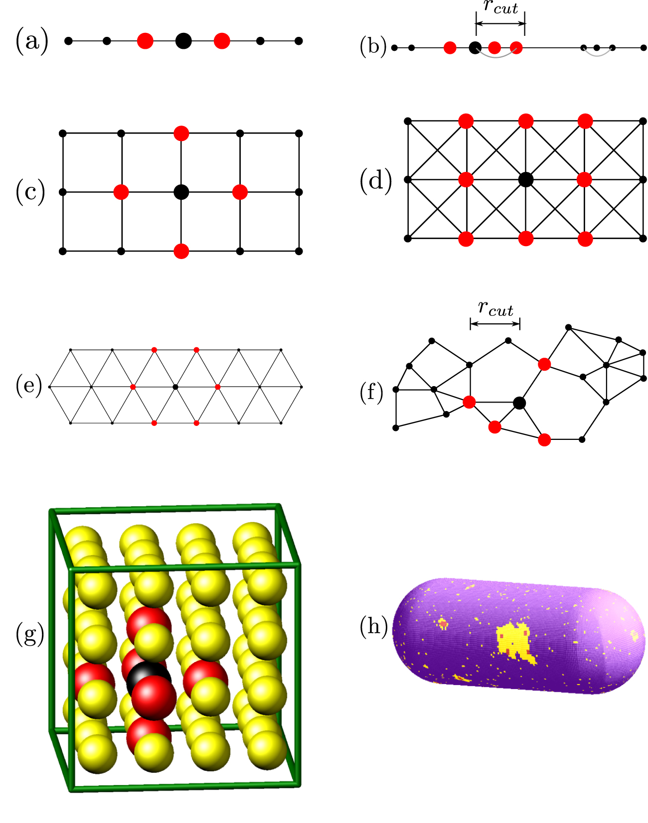
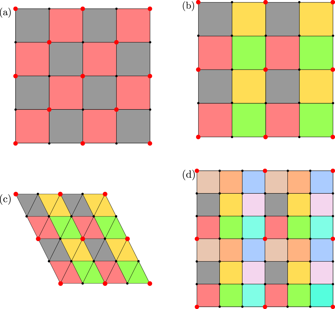
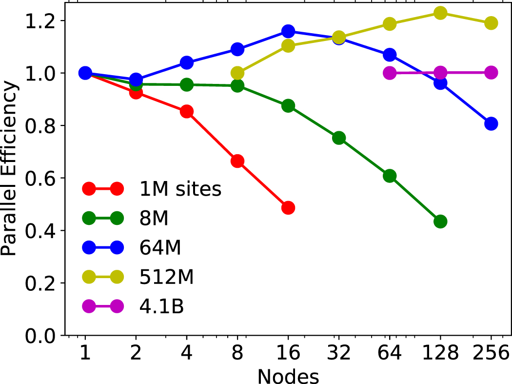
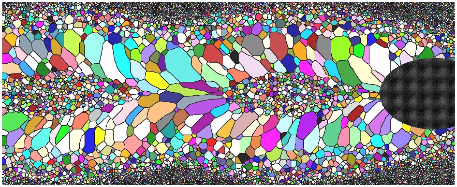
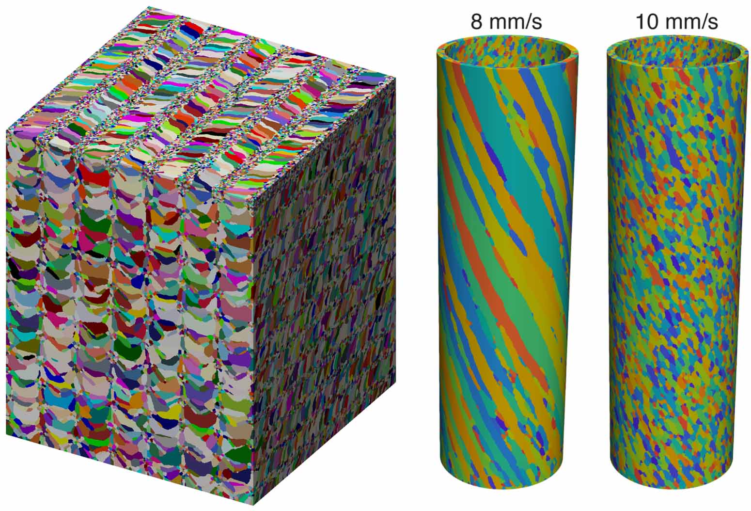
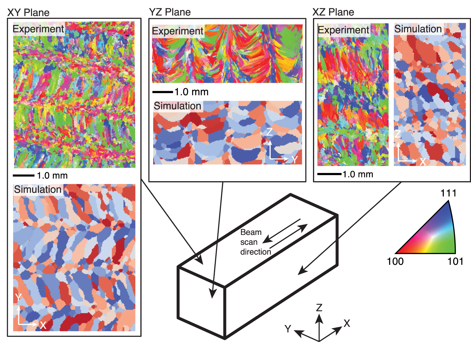
Figure 23. Simulation of a hybrid cellular automata and Potts model of recrystallization in UO2 nuclear fuel. (Left) Snapshots at different times (a)–(c) of evolving microstructure. (Right) Stored energy at the three times due to fission-induced damage within the same domain. Reprinted from [83], Copyright (2012), with permission from Elsevier.
Download figure:
Standard image High-resolution image
6. Summary and future work
We have described the functionality of the open-source SPPARKS code for performing parallel on-lattice Monte Carlo simulations via kinetic Monte Carlo (KMC), rejection KMC (rKMC), and Metropolis MC (MMC) algorithms. The code is designed to enable users to add their own, customized MC models. A variety of such models added by developers and users of SPPARKS were highlighted in section 5, all in the context of materials modeling or material processing simulations.
For parallel modeling, SPPARKS partitions the simulation domain so that each processor (MPI task) owns lattice sites (material) within a spatial subdomain. The synchronous sub-lattice (SSL) algorithm [12] is used to further partition subdomains into sectors so that MC events can be performed simultaneously on all the processors. However executing KMC, rKMC, or MMC algorithms in a spatially parallel manner makes them approximate versus the exact serial KMC algorithm. The different kinds of resulting approximation errors are detailed in section 2.9. Conceptually, the errors arise because parallelism includes some degree of spatial bias versus the exact serial algorithm which selects successive events randomly anywhere in the domain. This bias can result in boundary effects between sectors or undersampling or oversampling within sectors. An important feature of SPPARKS is that it has options to adjust its parallel algorithm to trade-off parallel efficiency versus accuracy for a particular model, as also discussed in section 2.9.
Three areas for possible future work or research with SPPARKS are outlined here. Namely, GPU acceleration, extended support for off-lattice models, and code coupling to enable multiphysics or multiscale models.
6.1. GPU acceleration
SPPARKS is currently a CPU-only code with support for distributed-memory parallel simulations via MPI. No threaded parallelism is implemented, either for CPUs (OpenMP) or graphical processing units (GPUs). One natural path to support this for MMC models are the coloring options described in section 2.7. Each MPI task can perform MC events simultaneously for sites it owns of the same color. However, the computational cost for a site to perform an event is quite small in most on-lattice models. It could thus require a very large number of sites per highly-threaded GPU to run efficiently.
For KMC or rKMC models, another idea is to implement the SSL algorithm and sectoring ideas of section 2.7 on a much finer scale, so that each MPI process has a large number of small sectored subdomains within its large processor subdomain. A similar strategy (for a single GPU) was proposed and tested in [84]. It also analyzed the effect of fine-grained sectoring on the fidelity of the simulation as compared to the exact serial KMC algorithm or the approximate coarse-grained distributed-memory SSL algorithm discussed in section 2.7.
6.2. Off-lattice algorithms
Limited SPPARKS support for off-lattice MC models was explained in section 2.13 and illustrated with a simple MMC energy minimization application. This model was relatively easy to implement in SPPARKS because the only off-lattice events included were small random displacements of individual atoms.
By contrast, consider an off-lattice atomic-scale diffusion model for a solid-state system, e.g. thin film growth due to deposition onto a free surface. In this context, MC diffusion events are hops by an atom from one energy-relaxed state to another. A specific conformation of a multispecies surface and substrate may have numerous point or extended defects induced by previous deposition events or by a strain-inducing lattice mismatch of the thin film with the substrate. There are at least three complex issues to consider for implementation of a fully functional off-lattice MC algorithm for this model.
First, identifying candidate locations to which each atom can potentially hop is non-trivial in an off-lattice model. In a KMC sense, accurately computing the barrier height (and thus relative propensity) for each diffusive hop requires a nudged-elastic band (NEB) [85] or similar calculation of the hop path which includes energy-relaxation of the system along the path, specifically at the saddle point of the barrier.
Second, diffusive events in such a system often do not only involve single-atom hops, but also multi-atom conformational changes. An example is the well-known exchange event [86] whereby a surface adatom moves into the substrate, inducing a substrate atom to move to a different adatom location on the surface. Such events also need to be identified and their energy barriers calculated to create a robust KMC model.
And third, as described in section 2.13, the energy equation used for off-lattice MC models involves an interatomic potential (or its analog for mesoscale models). There are a huge variety of analytic potentials appropriate for different materials and different combinations of materials (alloys, interfaces, etc). Increasingly, these include machine-learned potentials which are trained from large databases of quantum mechanical calculations such as density functional theory (DFT).
Some of these off-lattice capabilities could potentially be added to SPPARKS in a manner that allows for user-extensibility (e.g. to add a new interatomic potential). However a better strategy is likely to enable SPPARKS to be coupled to other materials modeling codes which provide complementary capabilities, either in a multiphysics (one scale) or multiscale sense. For example, the LAMMPS classical molecular dynamics package [36] implements a large number of interatomic and mesoscale potentials as well as a NEB capability. In a multiphysics context, it could be coupled to SPPARKS for atomic-scale diffusion applications such as the off-lattice thin film deposition model discussed above. See the next subsection for more discussion of code coupling with meso- and continuum-scale models.
The work by Joshi and Chaudhuri [57] mentioned in section 5.5 is an example of this approach. Another example, is the work of Martinez-Saez and Caro who coupled their own KMC code with two instances of LAMMPS to model diffusion-drive microstructural evolution (grain growth) [87]. The first instance of LAMMPS was partitioned into processor sub-groups to perform multiple NEB calculations simultaneously to compute diffusion barrier heights; the second instance was used to perform a global relaxation of the entire system after each KMC event was selected and performed.
6.3. Code coupling
In section 5.8, implementations of several hybrid MC + X applications were discussed, where X was a phase field, cellular automata, or PDE model (updated via finite-differencing). These were relatively simple to implement within the SPPARKS framework because the second model used the same underlying MC lattice and also required only local updates.
More generally in a multiphysics context, a second model may compute fields or other effects which are discretized at longer length scales or whose computation may be long-range (non-local) in nature. Examples include deformation, strain, or temperature fields, any of which can spatially influence the Hamiltonian used by an MC model. Examples of codes which calculate such fields are the VPFFT and CPFFT models for viscoplasticity (VP) and crystal plasticity (CP) effects on microstructure evolution in polycrystalline materials, which compute them via FFTs [88, 89]. A multiphysics MC + VP/CP model could potentially be developed by coupling SPPARKS with an existing VP or CP code, so that each could compute their portion of the hybrid model and exchange needed information each timestep.
Multiscale models which couple KMC or MMC models to continuum-scale solvers are another motivation for joining SPPARKS with an independent code. This is particularly attractive in the KMC context, since its timescale is determined by event rates, and it can thus naturally operate at multiple timescales.
In these contexts, we note that SPPARKS can be built as a library and has a simple C-style library interface (API) which allows another code or Python script to setup, invoke, and control one or more instances of a SPPARKS simulation. It also allows an umbrella code to invoke both SPPARKS and a second code (assuming it also has its own library interface) and to trigger the exchange of data between them.
New methods could be added to the SPPARKS library API to enable calls to lower-level functionality, aimed at supporting these more tightly coupled multiphysics or multiscale kinds of applications. In the same vein, support for use of SPPARKS with another code in a client/server mode of code coupling could also be added via use of the MolSSI MDI library [90, 91] designed to enable easy and flexible coupling of scientific simulation codes; see a discussion in [36] for how this was done for LAMMPS.
For use cases where both SPPARKS and another code partition the simulation domain spatially for parallel simulations and need to communicate large volumes of data (e.g. grid-based values), parallel data exchanges would be most efficient. A small, simple code-coupling library for communicating data in this manner is included in the SPPARKS distribution (examples/COUPLE directory). However, it could be enhanced for a variety of multiphysics and multiscale couplings, e.g. to infer mappings between different grid partitionings in the two codes, or to perform interpolation or upscaling between grids discretized at different resolutions.
Doing all of this work in the added context of creating CPU- and GPU-parallel efficient on-lattice or off-lattice KMC/rKMC/MMC models is an on-going research challenge. Our hope is that SPPARKS can be a useful tool not only as a stand-alone on-lattice MC code, but also for coupling to other materials modeling codes as well.
Acknowledgments
S J P and A P T wish to thank our friend and colleague Alex Slepoy, now deceased. He formulated the original plan to create SPPARKS, secured the necessary funding, and worked on its fundamental algorithms.
J A M gratefully acknowledges funding and support from the Advanced Certification and Qualification (ACQ) program within the DOE/NNSA.
E A H acknowledges support from the US National Science Foundation Grants CMMI-1826218 and DMR-2118945 and the United States Air Force D3OM2S Center of Excellence under Agreement FA8650-19-2-5209.
This work was originally supported by the Laboratory Directed Research and Development program at Sandia National Laboratories. The co-authors at Sandia are employees of National Technology & Engineering Solutions of Sandia, LLC under Contract No. DE-NA0003525 with the U.S. Department of Energy (DOE). As employees they own rights, titles and interest in and to the article and are responsible for its content. The United States Government retains and the publisher, by accepting the article for publication, acknowledges that the United States Government retains a non-exclusive, paid-up, irrevocable, world-wide license to publish or reproduce the published form of this article or allow others to do so, for United States Government purposes. The DOE will provide public access to these results of federally sponsored research in accordance with the DOE Public Access Plan; see www.energy.gov/downloads/doe-public-access-plan.
Data availability statement
The data that support the findings of this study are available upon reasonable request from the authors.
Footnotes
- 8
A similar on-the-fly visualization capability is implemented in two other particle-based codes which one of the authors (SJP) helped develop, namely LAMMPS [36] for molecular dynamics and SPARTA [37] for Direct Simulation Monte Carlo (DSMC) simulations. The parallel portion of the algorithm described in those papers is the same as described here for SPPARKS.
- 9
Laura Frink and Mark Stevens (Sandia National Laboratories) collaborated in formulating this AMP model.
- 10
Strong scaling is when the same-size system is run on more and more nodes.
- 11
Weak scaling is when the system size doubles each time the node count doubles.
- 12
An option is provided to only invoke the app_update() function and exclude the MC portion of the loop over sectors or sweep.