

Abstract
Managing heat through working fluids is essential in many applications, as well as the development of new fluids with improved properties. Therefore, the characterization of their thermal properties, which is usually a laborious task, is necessary to design and model new thermal systems. In this study, we show the proof of concept of a new method capable of determining the thermal conductivity, thermal diffusivity, and specific heat capacity of liquids from a single simple measurement, provided their density is known (a property easy to measure). The method is based on the use of a thermoelectric module, which is soldered to a large copper block at one side (heat sink). At the other side, the liquid is added on top of the ceramic external layer of the module. By means of impedance spectroscopy measurements, it is demonstrated for three liquids (water, Luzar, and diethylene glycol) that their thermal properties of can be obtained. In order to do this, a new equivalent circuit was developed to account for the new boundary conditions of the measuring setup. Random and systematic errors were calculated and combined to obtain a total uncertainty <8.6% for the thermal conductivity, <6.3% for the thermal diffusivity, and <6.1% for the specific heat capacity. The reasonably low uncertainties obtained position the new method as a low-cost alternative able to provide the three key thermal properties of liquids from one single measurement and only using a single setup.
Export citation and abstract BibTeX RIS

Original content from this work may be used under the terms of the Creative Commons Attribution 4.0 license. Any further distribution of this work must maintain attribution to the author(s) and the title of the work, journal citation and DOI.
1. Introduction
In our modern society, many applications require a working liquid to supply or remove heat, e.g. power generation stations, heating systems, or in refrigeration cycles. In some applications, it is necessary to model the behavior of the fluid and to select the right candidate to design new systems [1]. However, new working fluids are constantly being developed to protect their surroundings from corrosion [2] or to reduce the carbon footprint of their production or operation [3]. Therefore, those new fluids must be characterized before being used, and their thermal properties (such as the thermal conductivity, the thermal diffusivity and the specific heat) are especially important to know beforehand.
The most common characterization methods found in the literature to determine thermal properties of liquids are the parallel plates, concentric cylinders variable gap, transient hot wire, 3ω method, and laser flash. The parallel-plate and the concentric-cylinders methods are designed to represent as accurately as possible the ideal one-dimensional form of the Fourier law of heat conduction, where the heat flux and the temperature difference across the liquid are measured. These techniques are considered to be versatile and robust and, after a careful minimization of any heat leakages, the uncertainties can be <3% for the measurement of the thermal conductivity [4]. The variable-gap method is an attempt to mitigate the effects of convective and radiative losses by varying the distance between plates, especially important at high temperatures, but it uses the same steady-state working principle [5]. The transient hot wire is based on recording the temperature increase of a thin vertical metal wire when a voltage is applied to it [6, 7], and it is simple, quick, precise, and accurate for most electrical insulating liquids [8]. The 3ω method consists in measuring the third harmonic signal of a wire submerged in the liquid under evaluation, which is directly related to its thermal conductivity [9]. The laser flash technique measures the thermal diffusivity in a small amount of liquid, effectively eliminating convection effects, but it requires a specially constructed enclosure that increases its complexity [8]. Furthermore, a laser can also be used to determine the thermal conductivity of a liquid by measuring the interfacial thermal resistance [10]. However, this setup requires a thermal camera.
In a previous paper [11], we showed that impedance spectroscopy measurements on thermoelectric (TE) modules are sensitive to the thermal properties of a solid sample in contact with the module. We developed an experimental setup that related the total area underneath the complex plane plot (impedance response) with both, the thermal conductivity and the thermal diffusivity. Here, we develop a similar system adapted to liquid samples. In order to extract the thermal properties of the liquids by means of the impedance spectroscopy method, we have derived an equivalent circuit (theoretical model) that takes into account the different thermal processes in the new setup. This model can be used to perform fittings to the experimental impedance measurements, and directly obtain the thermal properties (thermal conductivity and thermal diffusivity). The specific heat of the liquid can also be determined by providing the mass density, which is a property easy to measure. Furthermore, the proposed method can be immune to corrosion and used with electrically conductive liquids since the liquid is only in contact with the outer ceramic surface of the TE module, and the recipient that contains the liquid can be fabricated with a non-corrosive material (e.g. stainless steel, plastic or ceramic).
2. Experimental setup
The main component of the experimental setup is a TE module from Custom Thermoelectric (ref. 07111-5L31-03CJ-T1), which has a number of TE couples N= 70, where each TE leg has a length L= 1.6 mm and a cross-sectional area A= 1.05 mm × 1.05 mm. The legs are connected by metallic strips of thickness LM= 0.3 mm, and held together by ceramic plates of LC= 0.7 mm thickness and 23 mm × 23 mm area. The ratio between the total area of the TE legs and the metallic strips is ηM = 0.56, and the filling factor (ratio between the total area of the TE legs and the area of the ceramic layer) is η = 0.26. To maintain the temperature constant during the impedance measurements, the bottom side of the TE module, which was tinned by the supplier with an In alloy, was soldered to a large copper block (10 cm × 10 cm × 5 cm). The soldering was performed by heating slowly the Cu block using a hot plate until the temperature at which the In alloy melts. It is important not to surpass too much this temperature to avoid melting the solder at the legs/metallic strips inside the TE module. Once the In alloy is melted pressure is applied with tweezers, the heating is switched off, and the TE module is let to cool down (while keeping the pressure until the alloy solidifies).
A container for the location of the liquid was created at the top ceramic layer of the TE module. For this purpose, a stainless-steel (AISI 304) frame of 0.3 mm wall thickness and external dimensions 21 mm × 21 mm with 3 mm height was fabricated. The frame was glued at the top part of the module with an adhesive (Loctite Super Glue-3), as shown in figure 1(a). Three different liquids were tested with different thermal conductivity values: distilled water (0.595 W (km)−1), Luzar Orgánico 50% (Carpemar, 0.404 W (km)−1) and diethylene glycol (MEGlobal, 0.242 W (km)−1). A volume of liquid of 1000 μl was added in all the measurements using a micropipette. Once added, the system was covered with a paper box to reduce convection losses (see figure 1(b)).

Figure 1. Photographs of the setup used (a) without and (b) with the paper box on top to reduce convection.
Download figure:
Standard image High-resolution imageImpedance measurements were performed with the setup inside a metallic vacuum chamber, which also acted as a Faraday cage, using an Autolab PGSTAT302N potentiostat equipped with a FRA32M impedance module and controlled using Nova 1.11.2 software. A total of 50 points separated logarithmically were recorded from 2 mHz to 100 kHz at a current amplitude of 20 mA, which was optimized as described in [12]. Briefly, this optimization consists in performing a few impedance measurements at different current amplitudes, and choosing a current just high enough to obtain the spectra free of noise. The measurements were performed using two minimum integration cycles in order to improve their repeatability. During all the measurements the ambient temperature, measured by a K-type thermocouple contacted on top of the copper block with thermal grease (see figure 1(a)), remained constant at 24.5 ± 0.5 °C.
3. Equivalent circuit
The equivalent circuit (theoretical model) used to fit the impedance spectroscopy measurements was obtained from solving the heat diffusion equation of the system with its different boundary conditions (see figure 2). This was performed using the thermal quadrupole method [13]. A similar equivalent circuit using this matrix-based method was developed in [14]. The main difference here is the addition of an additional layer (matrix) to account for the influence of the liquid at the top of the module, as it can be seen in figure 2.
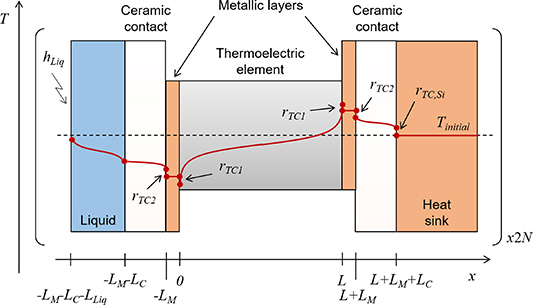
Figure 2. Schematic view (not to scale) of the experimental setup used in this study. The red line represents the temperature profile of a thermoelectric leg with positive Seebeck coefficient when a positive current is flowing through at a certain time, while the dashed line represents the temperature profile before the current is applied.
Download figure:
Standard image High-resolution imageAs shown in [14], the electrical impedance function, Z, as a function of frequency f, is given by,
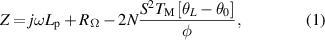
where j= (−1)0.5 is the imaginary unit, ω= 2πf denotes the angular frequency, Lp is the parasitic inductance, RΩ is the total ohmic resistance of the TE module, TM the ambient temperature, S is the Seebeck coefficient of each leg, and θL /φ and θ0/φ the thermal impedances at x= L and x= 0, respectively.
The thermal impedances θL /φ and θ0/φ are defined by,
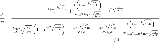
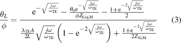
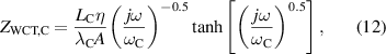
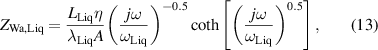
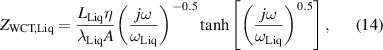
where ωTE= αTE/L2 is the characteristic angular frequency, and λTE and αTE are the thermal conductivity and diffusivity, respectively, of each TE leg. The parameters ZSi,M and ZLiq,M refer to the impedances toward the heat sink and liquid, respectively.
The impedance ZSi,M is defined as,
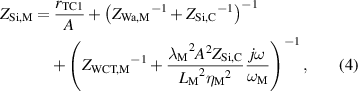
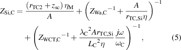
while, the impedance ZLiq,M is defined as,
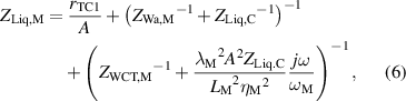
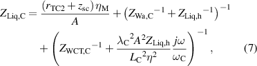
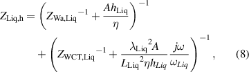
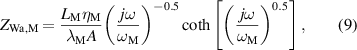
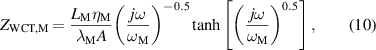
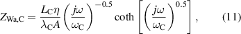
where rTC1, rTC2, and rTC,Si are the thermal contact resistivities between TE legs and metallic strips, between the metallic strips and ceramics, and between the bottom ceramic and heat sink, respectively. The thermal conductivity, thermal diffusivity, and characteristic angular frequency are λi, αi , and ωi = αi /Li 2, respectively, for the metallic strips i = M, ceramics i = C, and liquid i = Liq. The adiabatic and constant temperature Warburg elements of equations (4)–(8), are defined as,
and the parameter zsc, present in equations (5) and (7), is the spreading-constriction impedance, which takes the form [15],
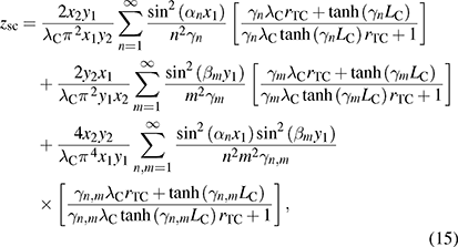
where rTC is the thermal contact resistivity at the outer ceramic surfaces (rTC= rTC,Si at the heat sink side, and rTC= 0 at the liquid side of the TE module). The constants αn = nπ/x2, βm = mπ/y2, γn = (αn 2 + jω/αC)1/2, γm = (βm 2 + jω/αC)1/2, and γn,m = (αn 2 + βm 2 + jω/αC)1/2 define all the possible solutions for the values n and m. The geometrical parameters x1= (A/η)1/2/2 + A1/2/2, x2= (A/η)1/2, y1= A1/2/2, and y2 = (A/η)1/2/2, are defined in the supplementary information of [15].
4. Results and discussion
Before characterizing the thermal properties of the liquid under evaluation, it was necessary to determine the thermal properties of the TE module, and the thermal contact resistance between the module and the copper block soldered at the bottom. To determine the thermal properties of the TE module, an impedance spectroscopy measurement with the module suspended in vacuum (at a pressure <10−4mbar) was performed. For this initial characterization, fixed values for αTE= 1.2mm2s−1, λM= 400Wm−1K−1, αM= 110mm2s−1, and αC= 10mm2s−1 were provided as temperature-independent constants in the fitting. A value of S= 212µVK−1 was also used in all fittings. It was directly measured by recording the voltage and temperature difference between the outer surfaces of the ceramics of the TE module in suspended and vacuum conditions when different constant current values were applied. Figure 3(a) shows the experimental impedance spectrum of the TE module suspended in vacuum (dots) and its fitting (line) using the MATLAB code provided in the supplementary information of [15]. From this first fitting, rTC1, λTE, and λC were determined (see table 1). It should be noted that rTC2 = 0 was found for this TE module, which was expected, since it is usual to find a good thermal contact between the metallic strips and ceramics. More information about this characterization procedure can be found in [14, 16].
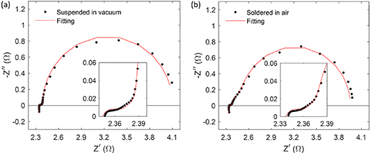
Figure 3. Measured impedance spectra (dots) obtained for the thermoelectric module (a) suspended in vacuum, and (b) after soldering to the copper block. The fittings in (a) and (b) were performed using the MATLAB codes provided in the supplementary information of [15] and of this manuscript, respectively.
Download figure:
Standard image High-resolution imageTable 1. Fitting parameters with the relative uncertainties in brackets of the impedance spectra shown in figure 3.
| Condition | Lp (H) | RΩ (Ω) | rTC1 (m2 KW−1) | λTE (Wm−1 K−1) | λC (Wm−1 K−1) | rTC,Si (m2 KW−1) |
|---|---|---|---|---|---|---|
| Suspended in vacuum | 1.53 × 10⁻⁷ (11.7%) | 2.34 (0.04%) | 1.21 × 10⁻⁵ (4.94%) | 1.53 (0.74%) | 24.4 (1.12%) | — |
| Soldered to Cu block in air | 1.69 × 10⁻⁷ (14.2%) | 2.33 (0.04%) | — | 1.67 (0.75%) | — | 2.05 × 10⁻⁴ (7.57%) |
After the TE module was characterized suspended in vacuum it was soldered to the copper block. A second impedance spectroscopy measurement was performed once soldered (in air, no vacuum) to determine the thermal contact resistance of the new copper block/bottom ceramic interface (rTC,Si). Figure 3(b) shows the experimental impedance spectrum of the soldered module (dots) and its fitting (line) using equation (1), which is implemented in the MATLAB code provided in the supplementary information. The fitting results can be seen in table 1. From this second fitting, rTC,Si was determined, and it was also fixed for the subsequent fittings (measurements with the liquids). It should be noted that λTE was not fixed for the second fitting, since the measurement was performed in air and it produces a small overestimation of this parameter [17]. Lp and RΩ were kept as free parameters in all measurements since they can have small variations every time that the wires of the setup are connected to the potentiostat.
Once the system with the TE module soldered was characterized, the stainless-steel frame was attached on the top side of the TE module and the cavity created was filled with the different liquids. Impedance measurements with and without the frame in air are shown in figure S1. It can be seen that some changes occur, however, they are less significant than the changes observed when the liquids are added (see the case for water in figure S1), thus, its influence is considered negligible. For each liquid, three impedance spectroscopy measurements were performed. A new volume of liquid was added for each measurement. Figure 4(a) shows the first impedance measurement performed with each liquid. It can be seen that the thermal properties of the liquid produce changes in the impedance response at intermediate-low frequencies. This is expected since the changes only appear when the frequency is low enough so that the Peltier heat flux reaches the interface between the ceramic of the TE module and the liquid. Lower frequencies than this point show a dependency on the thermal conductivity. A lower thermal conductivity of the liquid produces a more capacitive behavior at higher frequencies (see inset of figure 4(a)). The reason behind this is the accumulation of heat in the ceramic, which otherwise would diffuse into the liquid. The capacitive behavior is also observed for the other liquids, but it happens at lower frequencies (right part of the spectra).

Figure 4. (a) Measured impedance spectra of the experimental setup shown in figure 1 for the three liquids studied in this work. The symbols in (b), (c), and (d) show experimental data of water, Luzar, and diethylene glycol, respectively, while the lines show the fittings using the MATLAB code provided in the supplementary information. The value of the ohmic resistance (intercept with the real axis) has been removed from the real impedance data in (a) to improve the comparison.
Download figure:
Standard image High-resolution image
Figures 4(b)–(d) show the first of the three impedance spectroscopy measurements (symbols) for water, Luzar, and diethylene glycol, respectively. The lines are the fittings obtained with the MATLAB code provided in the supplementary information. It should be noted that the influence of the stainless-steel frame was neglected in the fittings, due to its small size. Also, the thermal contact resistance between the ceramic layer of the module and the liquid was not included in the fitting. Since the thermal conductivities of the ceramic and the liquids are medium and low, respectively, the resistance of this thermal contact is expected to be negligible [18]. In any case, we tried to perform fittings with a model that included the presence of a thermal contact between the ceramic of the TE module and the liquid and fittings were unsuccessful, pointing again to a negligible thermal contact resistance. It should be noted that in cases where this thermal contact resistance is not negligible, the fitting could provide its value, which is another interesting property that this method could obtain. For all nine fittings, the parameters Lp, RΩ, hLiq, λLiq, and αLiq were obtained. Their values can be found in table 2, together with the relative fitting uncertainty in brackets (estimated from the variance–covariance matrix). As it can be seen, the fitting uncertainty was mostly below 2% for the thermal conductivity (λLiq), and below 3% for all values of the thermal diffusivity (αLiq).
Table 2. Fitting parameters with the relative uncertainties in brackets of the three impedance spectra measurements (labeled as a, b, and c) for each of the three liquids studied in this work (water, Luzar, and diethylene glycol).
| Liquid | Measurement | Lp (H) | RΩ (Ω) | hLiq (Wm−2 K−1) | λLiq (Wm−1 K−1) | αLiq (m2 s−1) |
|---|---|---|---|---|---|---|
| Water | a | 4.24 × 10⁻⁷ (1.63%) | 2.33 (0.02%) | 33.1 (20.3%) | 0.566 (2.07%) | 1.43 × 10⁻⁷ (1.98%) |
| b | 4.26 × 10⁻⁷ (1.64%) | 2.33 (0.02%) | 28.5 (20.2%) | 0.538 (1.05%) | 1.31 × 10⁻⁷ (1.29%) | |
| c | 4.26 × 10⁻⁷ (1.63%) | 2.34 (0.02%) | 28.9 (20.6%) | 0.531 (1.17%) | 1.30 × 10⁻⁷ (1.48%) | |
| Luzar | a | 2.92 × 10⁻⁷ (3.50%) | 2.34 (0.02%) | 31.3 (17.5%) | 0.414 (1.13%) | 1.22 × 10⁻⁷ (1.56%) |
| b | 3.07 × 10⁻⁷ (2.20%) | 2.34 (0.02%) | 34.6 (16.9%) | 0.375 (0.94%) | 1.05 × 10⁻⁷ (1.49%) | |
| c | 3.08 × 10⁻⁷ (2.28%) | 2.33 (0.02%) | 30.9 (16.9%) | 0.417 (0.97%) | 1.21 × 10⁻⁷ (1.53%) | |
| Diethylene glycol | a | 4.14 × 10⁻⁷ (1.97%) | 2.35 (0.02%) | 35.7 (19.7%) | 0.253 (1.20%) | 9.31 × 10⁻⁸ (2.50%) |
| b | 4.07 × 10⁻⁷ (1.82%) | 2.35 (0.02%) | 33.2 (19.9%) | 0.249 (1.30%) | 9.41 × 10⁻⁸ (2.50%) | |
| c | 4.02 × 10⁻⁷ (2.05%) | 2.34 (0.02%) | 39.9 (19.1%) | 0.262 (1.26%) | 9.60 × 10⁻⁸ (2.84%) |
The mean values of thermal conductivity and thermal diffusivity for each liquid and their uncertainty can be found in table 3. The uncertainty in these two parameters was calculated considering two contributions: (i) the deviation between the measured values, ud [19], and (ii) the propagation of the error of the fitting uncertainties, up [20], as,
Table 3. Reference and measured thermal properties, their deviation, and the uncertainties for the three liquids studied. Reference values for water were extracted from literature [21], while specification sheets from the providers Carpemar [22] and MEGlobal [23] were used for Luzar and diethylene glycol, respectively.
| Liquid | Property | Reference | Measured (uc) | Deviation, us | Total uncertainty, ut |
|---|---|---|---|---|---|
| Water | dLiq (kg m−3) | 997 | — | — | — |
| λLiq (Wm−1 K−1) | 0.595 | 0.545 (2.04%) | −8.39% | 8.63% | |
| αLiq (m2 s−1) | 1.43 × 10⁻⁷ | 1.35 × 10⁻⁷ (2.95%) | −5.61% | 6.33% | |
| Cp,Liq (kJkg−1 K−1) | 4.18 | 4.06 (3.58%) | −2.90% | 4.61% | |
| Luzar | dLiq (kg m−3) | 1075 | — | — | — |
| λLiq (Wm−1 K−1) | 0.404 | 0.402 (3.00%) | −0.46% | 3.04% | |
| αLiq (m2 s−1) | 1.13 × 10⁻⁷ | 1.16 × 10⁻⁷ (4.33%) | 2.56% | 5.03% | |
| Cp,Liq (kJkg−1 K−1) | 3.33 | 3.23 (5.27%) | −3.07% | 6.10% | |
| Diethylene glycol | dLiq (kg m−3) | 1118 | — | — | — |
| λLiq (Wm−1 K−1) | 0.242 | 0.255 (1.68%) | 5.32% | 5.58% | |
| αLiq (m2 s−1) | 9.40 × 10⁻⁸ | 9.44 × 10⁻⁸ (1.75%) | 0.42% | 1.80% | |
| Cp,Liq (kJkg−1 K−1) | 2.30 | 2.42 (2.42%) | 4.87% | 5.44% |
where k1, k2 , and k3 represent the three measurements performed with the same liquid (they can be both parameters, the thermal conductivity or the thermal diffusivity), and uk1, uk2 , and uk3 represent their uncertainty, respectively.
Table 3 also shows reference values for thermal conductivity and thermal diffusivity, as well as for the specific heat capacity, Cp,Liq. The mass density, dLiq, was measured experimentally and it was used to calculate Cp,Liq, and its uncertainty, uc [20], as,
where uk Liq (k= λ or α) is the total uncertainty of the parameter k calculated as uk Liq 2 = ud 2 + up 2 using equations (16) and (17). The contribution to the uncertainty of the specific heat capacity from the experimentally measured mass density was neglected, since it is expected to be much lower than the other two contributions considered.
Finally, table 3 illustrates the systematic deviations between the measured and reference values, us, and the total uncertainty of the method, ut, calculated as ut 2 = uc 2 + us 2. Interestingly, no clear correlation between the systematic deviations and the property values was observed. In some cases, the total uncertainty was dominated by the random contribution while in other cases the systematic contribution was dominant. The fact that no obvious systematic overestimation or underestimation of the thermal properties was observed indicates that the assumption of a negligible influence of the thin stainless-steel frame is valid. Overall, the total uncertainty was <8.6% for the thermal conductivity, <6.3% for the thermal diffusivity, and <6.1% for the specific heat capacity, which are reasonably low values.
The working principle of the presented measuring system is similar to the 3ω method, however, the temperature increase in the sample is not due to Joule heating, but to the Peltier effect. In addition, the voltage variation is a consequence of the Seebeck effect, instead of the temperature coefficient of the resistance of the wire used in the 3ω method. Therefore, the method presented in this study has the potential to be more accurate than the 3ω wire thanks to measuring the 1st harmonic instead of the 3rd harmonic, and to recording a higher voltage amplitude for the same temperature increase in the sample. These advantages could allow measurements with a lower temperature increase in the liquid and, hence, minimizing convection errors.
5. Conclusions
A proof of concept of a new method to determine the thermal conductivity, thermal diffusivity, and specific heat capacity of liquids has been demonstrated. The technique consists on performing impedance spectroscopy measurements on a thermoelectric module, which is soldered at the bottom to a copper block. At the top, a thin frame is attached to locate the liquid samples. Impedance measurements before and after the soldering were used to characterize the properties of the module, and the thermal contact resistance between the module and the copper block. An equivalent circuit was developed to perform fittings to the impedance spectra obtained when the liquids are added. The proof of concept was demonstrated for three liquids: water, Luzar, and diethylene glycol, and the random and systematic uncertainties of their thermal properties were evaluated. The total uncertainty was <8.6% for the thermal conductivity, <6.3% for the thermal diffusivity, and <6.1% for the specific heat capacity. The new method developed offers the possibility to obtain these three key properties from a single and simple measurement, performed in only one setup, which can significantly facilitate the task and cost of characterizing the thermal properties of liquids.
Acknowledgments
This project has received funding from the European Union's Horizon 2020 research and innovation program under Grant Agreement No. 863222 (UncorrelaTEd project). Professor emeritus Ole Hansen (Technical University of Denmark) is also acknowledged for useful discussions.
Data availability statement
The data that support the findings of this study are openly available at Zenodo repository: https://zenodo.org/communities/uncorrelated/.
Matlab code (<0.1 MB zip)
Supplementary data (<0.1 MB DOCX)