
Abstract
Unsteady electrostatic forcing is investigated as a method for manipulating turbulent plasma behaviour within Hall-effect thrusters and similar cross-field plasma devices using a simplified one-dimensional three-velocity azimuthal electrostatic particle-in-cell simulation. A wide range of axial electric field forcing frequencies from 1 MHz up to 10 GHz at amplitudes of 10 V cm−1, 50 V cm−1 and 100 V cm−1 are applied to the plasma and the response is evaluated against a baseline case defined by the community benchmark LANDMARK Test Case 1. 'Tailoring' of plasma parameters, such as the electron cross-field mobility, is demonstrated via manipulation of the electron drift instability using unsteady forcing. Excitation of the unstable electron cyclotron modes by the electron drift instability is shown to be able to produce a reduction of the resultant electron cross-field mobility of the plasma by up to 50% compared to the baseline value. Additionally, forcing at the electron cyclotron frequency appears to be capable of increasing cross-field mobility by up to 2000%. Implications of the results for direct drive electric propulsion systems and improved current utilization efficiencies for Hall-effect thrusters are discussed.
Export citation and abstract BibTeX RIS

Original content from this work may be used under the terms of the Creative Commons Attribution 4.0 license. Any further distribution of this work must maintain attribution to the author(s) and the title of the work, journal citation and DOI.
1. Introduction
The Hall-effect thruster (HET), or stationary plasma thruster (SPT), is a form of electric propulsion (EP) system for spacecraft that generates thrust by accelerating the ions of a plasma using crossed electric and magnetic fields [1, 2]. The first Hall thruster flew in 1971 onboard the Soviet METEOR-18 satellite, which used two SPT-60 type thrusters for station-keeping manoeuvres [3]. Since then, HETs have evolved to become a mainstay of satellite EP technology. Between 2009 and 2018, over 43% of EP satellites launched into low Earth orbit have utilized some form of HET, whilst for geostationary Earth orbit satellites the percentage is even higher at 57% [3]. Despite their common use, the understanding of the underlying physics defining the systems operation has yet to be fully understood, particularly the ways in which turbulent plasma modes can affect performance [4]. Their design is informed, in many cases, by empirical scaling laws rather than self-consistent theory, making optimization a long, costly and primarily experimental process [5].
A typical HET consists of an annular ceramic channel, terminated by an anode at one end and left open at the opposite end, where a hollow cathode external to the channel is located [1, 2]. Ionized propellant is accelerated out of the thruster at high velocity, typically on the order of 10 km s−1 [1], by an axial electric field that imparts a small acceleration on the thruster. A strong magnetic field is applied radially, creating an E × B region that induces a Hall current on the electrons emitted by the cathode, confining them to the region of high magnetization and increasing their residence time in the channel [1]. Ions are generated by injecting a neutral propellant, usually xenon [5], at the anode, which is then ionized by the electrons trapped by the E × B drift. The large mass of the ions results in them being less affected by the E × B drift allowing them to freely accelerate out of the channel. HETs are typically described by cylindrical coordinates in three dimensions: the azimuthal dimension around the thruster channel, the radial dimension extending outwards radially from the inner magnetic coil and the axial dimension along the direction of the annular channel from the anode to the cathode end. A diagram showing the key features of the HET is shown in figure 1.

Figure 1. Diagram of an HET showing the principle of operation, curves Ez and By show axial electric field and radial magnetic field strength profiles, respectively, whilst Si shows the neutral ionization rate. E × B electron drift instability in Hall thrusters: particle-in-cell simulations vs theory. Reprinted from [6], with the permission of AIP Publishing.
Download figure:
Standard image High-resolution imagePlasma turbulence is a naturally occurring phenomenon that can lead to large discharge current oscillations within HETs and reduce the resultant current utilization efficiency of the propulsion system. Defining the discharge current supplied to a thruster  as the sum of the ion beam current
  and the electron current
  ,
,  . The 'useful' current supplied to the thruster is the ion beam current; therefore, we can define the current utilization efficiency as
From equation (1), it is evident that an increase in electron current results in a reduction of current utilization efficiency. One symptom of plasma turbulence within an HET is the so-called 'anomalous' electron cross-field mobility [7] observed when the number of electrons escaping the region of high magnetic field strength within the thruster channel is greater than that predicted by classical theory. This leads to higher discharge currents as  increases and reduced current utilization efficiency. There are several competing theories for the mechanism by which anomalous mobility occurs, such as secondary electron emissions from electron wall collisions [8, 9], sheath instabilities in radial direction due to secondary electron emission near the thruster channel walls [10, 11], gradient-driven fluid instabilities [12], and instabilities arising as a result of large azimuthal electron drift velocities, such as the electron drift instability (EDI) [13, 14]. Whilst the overall anomalous mobility experienced is fundamentally a result of the summation of all these effects, the instability-driven mechanism, via the EDI, is suspected to be dominant [15, 16].
Unsteady forcing is a widely explored technique in the field of aerodynamics for controlling nonlinear turbulent systems to improve the stall characteristics of airfoils at high angles of attack [17]. A chaotic system – for instance, a turbulent boundary layer or, in the case of this investigation, an unstable plasma – has a forcing signal applied to it (for example, pulsing air jets or, for a plasma, an oscillating electric field) with the goal of tailoring its macroscopic properties. Due to the natural energy pathways between wavemodes in the system, with the correct forcing, energy can be transferred between frequencies and wavenumbers in order to tailor the unsteady dynamics of the system to achieve structured or quasi-periodic behaviour from the chaos.
The primary aim of this study is to demonstrate tailoring of a macroscopic plasma property, the electron cross-field mobility, by manipulating microscopic plasma instabilities, such as the EDI, in a simplified computational model via the method of unsteady forcing. It is hoped that this analysis will provide a good basis for informing future work into improving the current utilization efficiencies and performance characteristics of HETs and adjacent cross-field plasma device technologies as a consequence of unwanted plasma dynamics. Examples of devices showing similar instabilities include magnetrons [18, 19] and tokamaks [20].
To the authors' knowledge, this is the first time manipulation of the EDI with unsteady electrostatic forcing has been attempted with the express goal of changing the resultant electron cross-field mobility in HETs. Previous works of interest on this topic aiming to manipulate the electron cross-field mobility include investigations by Bak et al [21, 22] into the effects of azimuthally inhomogeneous magnetic field and neutral gas supply, respectively, on the electron cross-field mobility. Further, Kapulkin and Prisnyakov [23] have previously investigated theoretical methods for suppressing the EDI by creating special grooves on the channel walls of an HET [23].
Other examples of where radiofrequency excitation of the electric field of a plasma has been used to demonstrate a significant quantifiable improvement in operation of a device include the work of Tejda et al [24]. In this study, excitation of the axial electric field of an HET led to an improvement in anode efficiency, thrust and specific impulse in computer simulation. In the past, Nishida et al [25] and Weiss and Morrone [26] have shown, both through experiment and theory, suppression of plasma drift waves in Q-machines using a high frequency applied electric field.
A derivation of the theoretical relationships describing the EDI and electron cross-field mobility are presented in the methodology along with a description of the numerical model. The results section outlines the steps taken to validate the model against the literature, followed by an investigation into the effects of unsteady electrostatic forcing over a range of frequencies and forcing amplitudes. Descriptions of the effects of forcing on the spectral amplitude distribution of the electric field are given and the electron cross-field mobility is evaluated. In the discussion, forcing frequencies at the frequency of the fundamental cyclotron harmonic are identified as resulting in a significant reduction in cross-field mobility, whilst forcing at the electron cyclotron frequency is shown to result in a significant increase. A theory is suggested to explain the observed reduction in cross-field mobility. Finally, in the conclusion the significance of the results are drawn with limitations of the model presented and avenues for further research identified.
2. Method
The theory underlining both the EDI and the electron cross-field mobility is outlined below in a simplified model for unbounded collisionless plasmas along with definitions of useful parameters for the subsequent investigation. The numerical model used to simulate these phenomena is then described along with the experiments performed to investigate the effects of unsteady forcing. The effect of unsteady forcing is quantified by first establishing a baseline case for the plasma where turbulence develops normally. This is then compared to the case with forcing applied and any change in the resultant plasma parameters are identified.
2.1. EDI
Also known as electron–cyclotron drift instability or beam cyclotron instability, the EDI is thought to be a primary factor in driving anomalous transport in HETs [15, 16]. Initially investigated in the context of collisionless longitudinal shocks in space plasmas in the 1960s and 1970s [6], the theory behind EDI formation is still an active topic of research. An EDI forms when electron Bernstein modes at high frequencies at multiples of the electron cyclotron frequency Doppler shift towards lower frequencies and the ion acoustic mode frequency range. Once within a similar frequency range, the two modes merge to form the EDI [27].
The dispersion relation, linking wavenumber k and frequency ω, for the EDI has been derived in both three dimensions and one dimension extensively by Ducrocq et al from the perturbed Vlasov equation [28]. Equation (2) shows the three-dimensional dispersion relationship
where g is the Gordeev function,  is the electron azimuthal drift velocity and
  is the primary axial ion beam velocity [29]. The wave number vector in three dimensions is
 ![$\mathbf{k} = [k_x,k_y,k_z]^\mathrm{T}$](https://content.cld.iop.org/journals/0022-3727/56/36/365203/revision2/dacd7f6ieqn8.gif) .
.  ,
,  ,
,  and
and  denote the Debye length, electron cyclotron frequency, the electron Larmor radius at thermal velocity
  and the ion plasma frequency, respectively.
Based on Ducrocq et al's analysis of equation (2) in the axial-azimuthal plane, it has been shown that the stability transitions for the EDI occur when  . For the EDI ω is small in comparison to
  , resulting in resonance peaks when
  ,
,  . The resultant unstable wavenumbers, the cyclotron harmonics, are denoted nk0 where
  [30]. In the limit where the wavenumber parallel to magnetic field is sufficiently large, such as for an HET with an appropriately sized radial dimension, the relation reduces to an ion acoustic-like dispersion relation with approximate analytical solution [12, 31, 32]
where ωR
and γ are the angular wave frequency and growth rate of the wave, respectively,  is the ion sound speed and
  and
and  are the ion and electron mass, respectively. Assuming the instability is primarily in the azimuthal dimension,
 ![$\textbf{k} \approx [k_{x}\, 0\, 0]^\mathrm{T}$](https://content.cld.iop.org/journals/0022-3727/56/36/365203/revision2/dacd7f6ieqn22.gif) and therefore
and therefore  . Setting
  finds k, ωR
and γ at maximum growth rate
finds k, ωR
and γ at maximum growth rate
The wave phase and group velocities are defined by  and
and  , respectively. From equation (3a
) we find for the EDI
, respectively. From equation (3a
) we find for the EDI

where  . Evaluating the EDI phase velocity at maximum growthrate we obtain
  .
.
2.2. Electron cross-field mobility
The electron cross-field mobility (also known as cross-field transport) describes the electron movement in the axial dimension out of the highly magnetized region of the thruster and is parameterized by  . The cross-field electron mobility is roughly analogous to the axial electron current. Electron cross-field mobility is predicted from the electron momentum conservation equation [33]
where  denotes the total derivative and
  the collision frequency of species α with species β. The flow velocity, electric and magnetic field strength, particle charge, density and pressure are denoted by u, E, B, q, n and p, respectively. Ignoring the pressure gradient and inertia terms in the axial and azimuthal directions, with a uniform magnetic field in the radial direction, B0, the momentum conservation equation becomes


Taking into account the presence of gradients and instabilities observed in the azimuthal direction of the thruster [34] and following the analysis of Lafleur [35], we calculate the effective cross-field transport parameter, taking average field quantities from the electron momentum conservation equations giving equation (9) where  is the electron-neutral collision frequency

For an even more detailed derivation of the cross-field mobility term, taking into account pressure gradient and inertia terms in the axial and azimuthal directions, see the work of Lafleur, Baalrud and Chabert [12, 31].
2.3. Description of the particle-in-cell (PIC) simulation
The underlying physics that govern the turbulent behaviour observed within HETs and the effects of unsteady forcing are outlined and modelled using a reduced-order one-dimensional three-velocity (1D-3 V) azimuthal fully kinetic electrostatic particle-in-cell (PIC) simulation code using Imperial College Plasma Propulsion Laboratory's (IPPL) PlasmaSim written in Julia [36]. Previous authors have concluded that an azimuthal 1D-3 V model is sufficient for capturing the plasma dynamics responsible for both the EDI development and the resultant anomalous electron mobility that is under investigation [37]. A simplified model of the HET reduces the complexity of the interactions between the many different plasma modes that exist in a real thruster, making analysing the links between the two properties under investigation far more tractable along with having a significantly reduced computational cost.
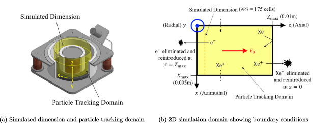
PIC simulation is a kinetic method for plasma simulation, representing electrons and ions as groups of 'super-particles' moving according to the particle equations of motion on a grid of cells used for calculating the statistical thermodynamic and electromagnetic properties within a plasma [38]. PlasmaSim has been validated for use in three 1D-3 V cases for the axial, radial and azimuthal directions of an HET, respectively, against other plasma models and experimental data [39]. The branch used in this investigation is derived from the azimuthal 1D-3 V electrostatic method popularized by Birdsall and Langdon [38] using the hard sphere model of Bird to model particle collisions [40]. Unless otherwise stated, it should be assumed that the PIC model is identical to that outlined by Birdsall and Langdon. The directions x, y and z denote the azimuthal, radial and axial directions of the HET, respectively, as shown in figure 2.
Download figure:
Standard image High-resolution imageGiven the technical complexity of producing a functioning PIC code, it is necessary to rigorously validate the results of any new code with respect to the available test cases and benchmarks provided by the community [7]. Furthermore, in order to identify the effects of applying unsteady forcing to the plasma, a suitable baseline simulation configuration to compare to had to be established. LANDMARK Test Case 1 [37] was identified as a suitable baseline for both validation and comparison purposes.
Figure 2(a) shows a diagram of the physical locations of the simulated dimension (dashed line), along which Poisson's equation is satisfied, and the particle-tracking domain (highlighted surface) in PlasmaSim on a reference SPT-100 thruster, reproduced with permission from Tejeda et al [24]. Figure 2(b) shows the two-dimensionalized version of the simulated dimension and particle tracking domain 'unwrapped' from the annular channel along with particle boundary conditions.
To accurately reproduce the baseline test case, the following boundary conditions were implemented for the particles and electric field. Wherever possible, the boundary conditions were chosen to replicate those used by Lafleur et al [35] to allow for a comparison of the results to those in the literature. Initially, electrons, neutrals and ions are all generated with a randomized Maxwellian thermalized velocity at a given temperature,  ,
,  and
and  , respectively, and randomized position within the particle-tracking region. Sizes of the super-particles are set according to specified number densities, n0 for electrons and ions and
  for neutrals. The azimuthal boundary condition is periodic, with Poisson's equation solved numerically using the finite difference method with Dirchelet boundary conditions of
  where particles passing outside the limits of
  or x < 0 are re-introduced at the same velocity on the other side of the domain. In order to simplify the modelling of the radial dimension of the HET, another periodic boundary condition was used which again reintroduced particles that left the extents of the simulation domain,
  or y < 0, on the other side of the domain. In the axial dimension, electrons passing out of the domain at the anode end (z = 0) were eliminated before being reintroduced at a random azimuthal location at the cathode end (
 ) with a thermalized velocity of temperature
  . The axial component of the velocity vector is enforced to be into the particle tracking domain to prevent hot electrons being eliminated straight after reinitialization. Similarly, for the ions, upon reaching the cathode end they are eliminated and reintroduced in a similar fashion at the anode end with temperature
  . Neutral particles are specularly reflected at the axial particle tracking boundary. The static electric and magnetic field strengths, E0 and B0, are set in the axial and radial directions, respectively.
Elastic collisions between charged particles and neutrals were captured in the model using the direct-simulation Monte Carlo method with expected particle collision frequencies between species α and β obtained using the hard sphere model of Bird, where the collision frequency  and the collision cross-section
  where r is the van der Walls radius of the colliding particle [40]. Ionization reactions between electrons and neutral particles were not captured as part of the model.
Given the statistical nature of PIC simulation, Julia's [36] inbuilt random number generator using the Xoshiro256++ algorithm is used to generate independent trial runs for each scenario using a different random number generator seed before averaging to remove the effects of statistical noise. Limitations on the simulation parameters for the spatial discretization of the modelled dimension ( ) are given by the requirement that
  must be less than
  to resolve the Debye length of the plasma and not simply capture collective effects. The time step of the simulation is required to resolve both the electron plasma (
 ) and cyclotron frequency (
 ) from the Nyquist criterion, and satisfy the Courant–Freidrichs–Lewey condition (
 ) which are given by below [38]


An additional safety factor of 25 is then applied to the minimum time step.
The electron cross-field mobility parameter can be calculated numerically from the simulation particles by evaluating the average axial velocity of the electrons according to equation (11) where N is the number of electron super-particles at each time step.
2.4. PIC simulation baseline definition
The key publications laying out the conditions and expected results of the baseline configuration are given in 'Nonlinear structures and anomalous transport in partially magnetized E × B plasmas' by Janhunen et al [30] and 'Theory for the anomalous electron transport in Hall effect thrusters I & II' by Lafleur et al [32, 35], which were used in the validation of the results obtained by PlasmaSim. The baseline plasma properties used for the initialization of the simulation are given in table 1. Where possible, the values of the plasma properties were selected to be identical to those used by Lafleur et al [35] to validate the results generated by PlasmaSim against the results available in the literature. The neutral number density was arbitrarily selected so that the neutral gas pressure would be sufficiently low to observe the instability [35].
Table 1. Baseline operating and numerical parameters used in the PIC simulations.
| Plasma property | Value |
|---|---|
 (eV) (eV) | 2.0 |
 (eV) (eV) | 0.1 |
 (K) (K) | 300 |
| B0 (T)] | 0.02 |
| E0 (V cm−1) | 200 |
 (m−3) (m−3) |

|
| n0 (m−3) |

|
Simulation parameters such as the time step, data capture frequency and spatial discretization were tuned to satisfy the conditions given by equations (10a
)–(10d
) to reduce numerical inaccuracy of the model and achieve an accurate depiction of the EDI and cross-field mobility development. The final simulation parameters settled on are shown in table 2. Again, where possible, the baseline simulation parameters were chosen to closely resemble those used by Lafleur et al [35]. Results from a mesh-refinement study confirmed that a sufficient number of cells (NG) for resolving the instability was 175 in the x dimension with a time step (tstep) of  s. A data capture rate (twrite) of
  s was selected by Nyquist's criterion to capture interesting plasma behaviour at frequencies up to and including the electron plasma frequency whilst reducing the size of the simulation output files. The extents of the simulation domain Xmax, Ymax and Zmax were chosen as 0.005 m, 0.0075 m and 0.01 m, respectively. One hundred super particles per cell for each species (
 ) were selected from the literature as an appropriate number for initialization of the simulation.
Table 2. Simulation parameters.
| Simulation parameter | Value |
|---|---|
| tstep (s) |

|
| twrite (s) |

|
| NG | 175 |

| 100 |
| Xmax (m) | 0.005 |
| Ymax (m) | 0.0075 |
| Zmax (m) | 0.01 |
2.5. Application of unsteady forcing
The primary method to affect unsteady forcing was by varying the axial electric field, which was thought could provide a mechanism for manipulating azimuthal instabilities and hence the cross-field mobility of the plasma. It has previously been observed that forcing the axial electric field can lead to changes in the temporal spectral energy distribution of the azimuthal electric field; however, specific effects of forcing over a wide band of forcing frequencies have yet to be fully characterized.
In a real HET, axial electric field forcing can be accomplished by varying the potential of the anode or the cathode to achieve the desired electric field. This has previously been suggested by Tejeda et al [24] but not yet been tested experimentally. The axial electric field in an HET is non-uniform, as shown in figure 1, but, given that the 1D-3 V azimuthal version of PlasmaSim does not resolve Poisson's equation in this direction, the axial electric field profile is instead simplified to a uniform field varying in time with field strength given by  , where E0 is the average static electric field strength and
  is the superimposed oscillation. AEF is the amplitude and
  is the frequency of the forcing of the electric field, t is the simulation time.
3. Results
3.1. Simulation validation
The plasma distributions obtained in PlasmaSim for the parameters specified for the baseline test case are shown in figure 3. Both the electron density and the azimuthal electric field show wave-like behaviour with high wavenumber oscillations over the first 500 ns giving way to low-wavenumber, progressively more chaotic, high-amplitude oscillations as the instability saturates towards 4000 ns.

Figure 3. (a) Normalized electron number density 
 and (b) azimuthal electric field strength
  for baseline test case parameters.
Download figure:
Standard image High-resolution imageThe wavenumber and frequency of the wave-like behaviour can be calculated from the electric field distribution by counting peaks along lines XX and YY of figure 4 respectively after saturation. The wave phase velocity can be evaluated from  . This method gives a wave phase velocity of
  m s−1 , wave number of
  rad m−1 and a frequency of
  rad s−1. Given the electron temperature at 4500 ns is approximately
  the Debye length of the plasma would have increased to
  m. Using equations (4a
), (4b
) and (6), we calculate the expected wavenumber at maximum growth rate
m. Using equations (4a
), (4b
) and (6), we calculate the expected wavenumber at maximum growth rate ![$[k]_\mathrm{max}$](https://content.cld.iop.org/journals/0022-3727/56/36/365203/revision2/dacd7f6ieqn75.gif) at 4500 ns of
at 4500 ns of  rad m−1, frequency
 ![$[\omega_R]_\mathrm{max}$](https://content.cld.iop.org/journals/0022-3727/56/36/365203/revision2/dacd7f6ieqn77.gif) of
of  rad s−1 and phase velocity
 ![$\text{v}_\phi([k]_\mathrm{max})$](https://content.cld.iop.org/journals/0022-3727/56/36/365203/revision2/dacd7f6ieqn79.gif) of
of  m s−1 for the EDI. The results show good agreement with those obtained from the analytical dispersion relationship for the wavenumber of maximum growth rate. Phase velocity, wavenumber and frequency show a 2.8%, 11.7% and 0.5% error from the theoretical values, respectively. This was deemed to be within acceptable bounds given the assumptions of the theoretical model of an unbounded collisionless plasma and suggests PlasmaSim is accurately modelling the expected physics of the EDI. k, ω and
  of the resultant wave behaviour appears to be closely related to the wavenumber of maximum growth rate
 ![$[k]_\mathrm{max}$](https://content.cld.iop.org/journals/0022-3727/56/36/365203/revision2/dacd7f6ieqn82.gif) .
.
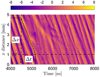
Figure 4. Normalized azimuthal electric field strength  distribution annotated to calculate wavenumber, frequency and wave speed of the resultant wave-like behaviour.
Download figure:
Standard image High-resolution imageIt should be noted that in the numerical model both the electron temperature and electron number density oscillate between approximately  and
and  , and
, and  m−3 and
  m−3, respectively, after the instability saturates. The values of the phase velocity, wavenumber and frequency calculated from equations (4a
), (4b
) and (6) do not account for these oscillations, using instead the instantaneous values for electron temperature and number density at 4500 ns of
m−3, respectively, after the instability saturates. The values of the phase velocity, wavenumber and frequency calculated from equations (4a
), (4b
) and (6) do not account for these oscillations, using instead the instantaneous values for electron temperature and number density at 4500 ns of  and
and  m−3, respectively. This is a likely explanation for the remaining discrepancy between the numerically calculated wavenumber and the theoretical value as the theoretical value is sensitive to these parameters.
The dispersion relationship of the EDI was calculated numerically by taking a two-dimensional fast Fourier transform of the azimuthal electric field from PlasmaSim in MATLAB [41] to convert it to a wavenumber–frequency diagram, as shown in figure 5. The numerical and analytical dispersion relationships show good agreement, with the wavenumber of the largest growth rate in figure 5 being close to the analytically calculated value of ![$[k]_\mathrm{max}$](https://content.cld.iop.org/journals/0022-3727/56/36/365203/revision2/dacd7f6ieqn90.gif) and
and ![$[\omega_R]_\mathrm{max}$](https://content.cld.iop.org/journals/0022-3727/56/36/365203/revision2/dacd7f6ieqn91.gif) for the EDI from equations (4a
) and (4b
). These results were compared to Lafleur et al's [12] results finding the same dispersion relationship despite Lafleur et al using a 2D-3 V axial–azimuthal PIC model. This gives confidence in the one-dimensional model retaining enough complexity to model the EDI sufficiently despite the dimensionality reduction.
for the EDI from equations (4a
) and (4b
). These results were compared to Lafleur et al's [12] results finding the same dispersion relationship despite Lafleur et al using a 2D-3 V axial–azimuthal PIC model. This gives confidence in the one-dimensional model retaining enough complexity to model the EDI sufficiently despite the dimensionality reduction.
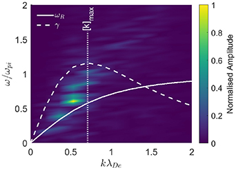
Figure 5. Wavenumber–frequency diagram for wave-like behaviour exhibited by azimuthal electric field showing the contour of a numerically obtained dispersion relationship and a dashed line showing the predicted analytical dispersion relationship from equation (3a ) (growth rate γ scaled by a factor of 12).
Download figure:
Standard image High-resolution imageThe electron cross-field mobility calculated from equation (11) and averaged over the time period after instability saturation (6 µs–10 µs) was found as 5.38 m2 V−1 s−1. To reduce the effects of statistical variation, the result was averaged over five independent simulation runs with a standard deviation of 0.94 m2 V−1 s−1, agreeing with the cross-field mobility parameter obtained by Lafleur [35] for similar simulation parameters.
3.2. Effect of unsteady forcing
Initial investigations focused on applying forcing at frequencies at or near the fundamental plasma frequencies, the electron cyclotron frequency  , the electron plasma frequency
  and the ion plasma frequency
  . Three forcing amplitudes AEF of 10 V cm−1, 50 V cm−1 and 100 V cm−1 were tested. The resulting cross-field mobility increased significantly from the baseline value by up to a factor of 20 times when forcing at the electron cyclotron frequency with the largest increase at a forcing amplitude of 100 V cm−1 and the smallest increase at an amplitude of 10 V cm−1. Only a small increase in cross-field mobility was noted when forcing at the electron plasma frequency, as shown in figure 6; however, this was not judged to be statistically significant. A slight reduction in cross-field mobility was observed forcing at the ion plasma frequency; however, this was only statistically significant at a forcing amplitude of 50 V cm−1.

Figure 6. Electron cross-field mobility of plasma for  of specified plasma fundamental frequency at specified forcing amplitudes
  where error bars and dashed red line show one standard deviation from the value.
Download figure:
Standard image High-resolution imageThe temporal spectral amplitude distribution for the azimuthal electric field was compared with the baseline distribution for each forcing frequency. To reduce the effects of statistical noise, the amplitude spectrum for the baseline test case was averaged over five independent simulation runs to obtain the expected distribution whilst the amplitude spectrum for the forced case was averaged over three independent runs. Significant divergences from the baseline distribution were identified for forcing frequencies matching the electron cyclotron frequency and the ion plasma frequency, as can be seen from figures 7 and 8, respectively. Forcing at the electron cyclotron frequency resulted in a reduction in spectral amplitude around the frequency of maximum growth rate of the EDI ![$[\omega_R]_{\mathrm{max}}$](https://content.cld.iop.org/journals/0022-3727/56/36/365203/revision2/dacd7f6ieqn97.gif) whilst all other frequencies saw an increase in amplitude, particularly for frequencies exceeding the 'so-called' Hall circulation frequency
whilst all other frequencies saw an increase in amplitude, particularly for frequencies exceeding the 'so-called' Hall circulation frequency  where
where  is the drift velocity
  . Conversely, forcing at the ion plasma frequency leads to an increase in spectral amplitude for frequencies between
  and ωE with a reduction in the spectral amplitude for frequencies greater than ωE or lower than
  , the amplitude of the peaks associated with the electron cyclotron frequency and its resonances appeared to be damped when forcing at this frequency was applied.
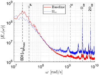
Figure 7. Azimuthal electric field spectral amplitude distribution of the baseline case compared to the forced case at electron cyclotron frequency with  of 100 V cm−1.
Download figure:
Standard image High-resolution image
Figure 8. Azimuthal electric field spectral amplitude distribution of the baseline case compared to the forced case at ion plasma frequency with  of 100 V cm−1.
Download figure:
Standard image High-resolution imageTo attempt to fully characterize the effects of unsteady forcing, a wider range of frequencies from the MHz range up to the GHz range were investigated. Simulations were run with forcing frequencies  from
from  Hz to
Hz to  Hz in logarithmic steps, i.e 106 Hz, 106.1 Hz, 106.2 Hz etc, to encompass the whole range. Again, three forcing amplitudes
  of 10 V cm−1, 50 V cm−1 and 100 V cm−1 were tested to quantify the effects of varying forcing amplitude. The resultant power spectrum data and associated cross-field mobility were averaged over three independent simulation runs similarly to above.
Approximate forcing effects can be grouped roughly according to the qualitatively observed effects in different frequency bands. To aid discussion, the 'low' frequency band shall be frequencies below the ion plasma frequency  , 'mid-range' frequencies shall be between
  and the Hall circulation frequency
  and 'high' frequencies shall be frequencies above the Hall circulation frequency. Forcing frequencies
  in the low frequency range, below the ion plasma frequency, typically resulted in spectral amplitude reduction in the low frequency range, as demonstrated in figure 9. Furthermore, above
  , the spectral amplitude showed a characteristic reduction, particularly around the electron cyclotron frequency resonances and the Hall circulation frequency. No obvious resonant behaviour was observed at multiples of the forcing frequency in this range.

Figure 9. Azimuthal electric field spectral amplitude distribution of the baseline case compared to the typical forced case in the low-frequency range ( Hz) with
  of 50 V cm−1.
Download figure:
Standard image High-resolution imageMid-range forcing for  between the ion plasma frequency
  and the Hall circulation frequency
  resulted in interesting behaviour whereby large peaks in amplitude centred on the forcing frequency
  and its resonances appear in the spectral amplitude distribution for the azimuthal electric field. An example of this behaviour is shown in figure 10, demonstrating a coupling between the axial and azimuthal electric field behaviour. Mid-range forcing also appears to reduce the spectral amplitude in both the high- and low- frequency ranges. As the forcing frequency approaches
  , the amplitude of the electron cyclotron peak and its resonances become increasingly damped, potentially indicating a coupling between the mid-range frequency modes and the high frequency electron cyclotron modes.
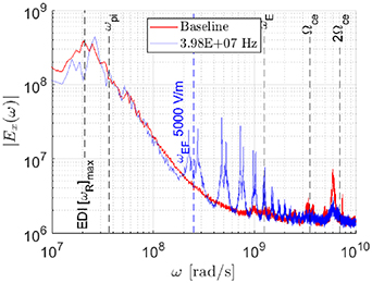
Figure 10. Azimuthal electric field spectral amplitude distribution of the baseline case compared to the typical forced case in the mid-frequency range ( Hz) with
  of 50 V cm−1.
Download figure:
Standard image High-resolution imageFigure 11 shows a characteristic response of the plasma when forced within the high-frequency range, demonstrating the observed phenomena of 'frequency lock-in'. When the plasma is forced at a frequency close to the electron cyclotron frequency, the peak typically located at  is observed to shift slightly away from its usual position towards the forcing frequency or lock-in frequency. Similar behaviour is observed at the resonances of the electron cyclotron frequency, sometimes with a significant amplitude reduction or peak sharpening at the other resonances. When
  is not located near an electron cyclotron frequency resonance, no significant change in the spectral amplitude distribution is observed. Forcing close to the Hall circulation frequency
  and its resonances appears to amplify the other Hall circulation resonances.
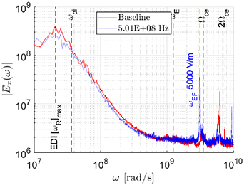
Figure 11. Azimuthal electric field spectral amplitude distribution of the baseline case compared to the typical forced case in the high-frequency range ( Hz) with
  of 50 V cm−1.
Download figure:
Standard image High-resolution imageGenerally speaking, increasing the amplitude of the forcing function appears to increase the change in the observed spectral amplitude. Forcing at 10 V cm−1 does not appear to significantly reduce the low-frequency spectral amplitude compared to forcing at 50 V cm−1 when  is in the low-frequency range. When
  is in the mid- to high-frequency region, the response for 10 V cm−1 amplitude is similar to that observed for the higher forcing amplitudes tested.
The cross-field mobility calculated for the plasma at each forcing condition over a range of frequencies is shown in figures 12–14 for forcing amplitudes of 10 V cm−1, 50 V cm−1 and 100 V cm−1, respectively, and compared to the expected value calculated from the unforced baseline case. Taking into account the statistical variation in the result output by the PIC algorithm, the figures show both the mean value and the region of one standard deviation from the mean. The mean baseline cross-field mobility is represented by a horizontal red line with the standard deviation of this shown by two dashed horizontal red lines. Statistically significant results that showed a deviation of the cross-field mobility from the baseline value were identified using a two-sample, two-tailed t-test at the 5% confidence level and are circled in red.
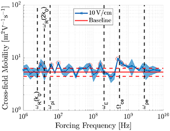
Figure 12. Cross-field mobility of plasma excited at a given forcing frequency  at a forcing amplitude
  of 10 V cm−1.
Download figure:
Standard image High-resolution image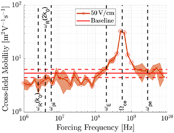
Figure 13. Cross-field mobility of plasma excited at a given forcing frequency  at a forcing amplitude
  of 50 V cm−1.
Download figure:
Standard image High-resolution image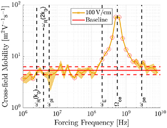
Figure 14. Cross-field mobility of plasma excited at a given forcing frequency  at a forcing amplitude
  of 100 V cm−1.
Download figure:
Standard image High-resolution imageAs expected from the prior investigation of plasma fundamental frequencies, for all three forcing amplitudes tested the cross-field mobility peaks when the forcing frequency is close to  with cross-field mobility increasing with amplitude. There is a reduction in cross-field mobility by a factor of up to a half relative to the baseline test case for forcing frequencies close to the frequency of the fundamental cyclotron harmonic
  and its resonances; this is most pronounced for a forcing amplitude of 50 V cm−1. At the same forcing amplitude, the cross-field mobility appears to be reduced somewhat for forcing frequencies in the range between the ion plasma frequency and the Hall circulation frequency, and no such effect is distinguishable for the other trial forcing amplitudes. Forcing at 10 V cm−1 appears to result in the smallest deviation in cross-field mobility to the baseline case for low- and mid-range frequencies.
4. Discussion
4.1. Significance of frequency of cyclotron harmonics
The reduction in cross-field mobility in the low frequency range is centred upon the frequency of the EDI's unstable cyclotron harmonics  The frequencies of these harmonics are calculated from the dispersion relationship for the EDI from the equation of angular wave frequency (3a
). Substituting in the unstable cyclotron wavenumbers nk0 to this equation gives the wave frequency as
The frequencies of these harmonics are calculated from the dispersion relationship for the EDI from the equation of angular wave frequency (3a
). Substituting in the unstable cyclotron wavenumbers nk0 to this equation gives the wave frequency as

where  and
and  is a function of the electron temperature. Forcing at the frequency
  was observed to reduce the temporal spectral amplitude of frequencies other than those corresponding to an unstable wavemode in the low frequency region, potentially as a result of energy pathways amplifying the unstable EDI mode or as a result of frequency lock-in type behaviours. Figure 15 demonstrates this behaviour for forcing at the frequency of the fundamental cyclotron harmonic
  for the temporal spectral distribution. Observing the region of the spectrum between
  rad s−1 and
  rad s−1, the spectral amplitude for the forced plasma shows peaks at
  ,
,  and
and  with a reduction in spectral amplitude everywhere else compared to the baseline case. Similar results were observed for cases where forcing is applied at the frequencies of two other unstable cyclotron harmonics
  and
and  .
.
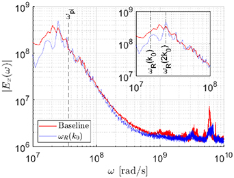
Figure 15. Azimuthal electric field temporal spectral amplitude distribution of baseline case compared to case forced at fundamental cyclotron frequency k0 with  of 50 V cm−1.
Download figure:
Standard image High-resolution imageComparing the development of the spatial spectral amplitude distribution for the azimuthal potential field of the baseline case shown in figure 16 with that forced at the frequency of the fundamental cyclotron harmonic  shown in figure 17, it can be seen that forcing induces a reduction in spectral amplitude for wavemodes that are not excited,
  ,
,  , whilst the excited wavemode k0 sees an increase in amplitude. Counterintuitively, we see a reduction not an increase in cross-field mobility by forcing at the frequency of the unstable modes of the EDI. Referring back to equation (9), it is known that the cross-field mobility is dependent on the cross-correlation term
  . Calculating this term for the baseline case and comparing it with the calculated term for the forced case at the frequency of the fundamental cyclotron harmonic at 50 V cm−1 shows a reduction of over 50% for the forced case. One possible theory for the reduction could be due to the forcing causing Ex
and
. Calculating this term for the baseline case and comparing it with the calculated term for the forced case at the frequency of the fundamental cyclotron harmonic at 50 V cm−1 shows a reduction of over 50% for the forced case. One possible theory for the reduction could be due to the forcing causing Ex
and  to oscillate out of phase, reducing
  and the resultant cross-field mobility.

Figure 16. Development of plasma azimuthal potential field spatial spectral amplitude distribution of the baseline case over the first 4 µs of simulation time with  of 50 V cm−1.
Download figure:
Standard image High-resolution image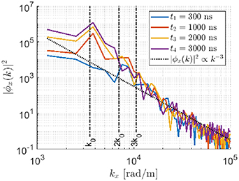
Figure 17. Development of azimuthal potential field spatial spectral amplitude distribution of plasma forced at fundamental cyclotron frequency  over the first 4 µs of simulation time with
  of 50 V cm−1.
Download figure:
Standard image High-resolution image
It was observed from the spatial Fourier transform of the potential field that  , as illustrated in figure 16. This establishes an energy–wavenumber relationship seemingly similar to those predicted by Kolmogorov cascade theory whereby a turbulent field's spectral amplitude is proportional to k−n
where n is a constant to be determined [42, 43]. The
, as illustrated in figure 16. This establishes an energy–wavenumber relationship seemingly similar to those predicted by Kolmogorov cascade theory whereby a turbulent field's spectral amplitude is proportional to k−n
where n is a constant to be determined [42, 43]. The  relationship has been observed to hold for instabilities in tokamak fusion plasmas studied by Qi [44], although more work is required to determine if there is any applicable similarity to tokamak instabilities here that could also be exploited for HETs and on the significance of the
  relationship overall.
4.2. Significance of the electron cyclotron frequency
Forcing close to the electron cyclotron frequency led to a large increase in cross-field mobility. It is theorized that this could be a result of disruption to the circular motion of the electrons normally oscillating at that frequency in the E × B field, causing the electrons to break confinement. Whilst promoting the electron mobility classically would seem to be a detriment to HET systems, due to the reduction in current utilization efficiency, it could also be a pathway to reducing the anode voltage of such a system, enabling the possibility of a direct drive architecture.
5. Conclusion
Unsteady forcing of the axial electric field was successfully demonstrated as a method for manipulating plasma turbulence within the azimuthal electric field of a cross-field E×B device in simulation using a reduced-order 1D-3 V electrostatic PIC model. Wider characterization of the effects of unsteady forcing on the baseline test case for frequencies between  Hz and
  Hz at three different forcing amplitudes, 10 V cm−1, 50 V cm−1 and 100 V cm−1 was carried out. This led to a conclusion that a link between the electron cyclotron frequency
  and the frequency of maximum growth rate of the EDI
 ![$[\omega_R]_\mathrm{max}$](https://content.cld.iop.org/journals/0022-3727/56/36/365203/revision2/dacd7f6ieqn166.gif) exists; indicated by a reduction of the temporal spectral amplitude corresponding to
exists; indicated by a reduction of the temporal spectral amplitude corresponding to ![$[\omega_R]_\mathrm{max}$](https://content.cld.iop.org/journals/0022-3727/56/36/365203/revision2/dacd7f6ieqn167.gif) for the EDI when forcing at the electron cyclotron frequency
for the EDI when forcing at the electron cyclotron frequency  and vice versa. Investigating the effects on azimuthal electric field spectral response to a forcing frequency three main frequency bands were identified: forcing within the range
  led to a spectral amplitude reduction in the range
  to
to  . Forcing in the range of frequencies
  resulted in a peak in spectral amplitude at the forcing frequency and its harmonics and a spectral amplitude reduction in the range
  . Damping of the peak corresponding to the electron cyclotron frequency was observed as the forcing frequency approached
  . Forcing in the range
  demonstrated frequency 'lock-in' behaviour that was observed for forcing frequencies close to the electron cyclotron frequency. Forcing in this range also resulted in amplification of the spectral amplitude of the peaks corresponding to the Hall circulation frequency and its resonances when forcing at said frequency.
The electron cross-field mobility was evaluated and compared to the baseline value for each forcing frequency. It was found that forcing at the frequency of the fundamental cyclotron harmonics  resulted in a significant reduction in cross-field mobility. A theory for the reduction was presented whereby the reduction in cross-field mobility could result from forcing causing the electric field and the electron density distribution to oscillate out of phase with one another, reducing the resultant cross-field mobility. Conversely, forcing at frequencies close to the electron cyclotron frequency led to a significant increase in cross-field mobility, thought to be as a result of disruption to the circular motion of the electrons in the E × B field.
Future areas of interest diverging from these findings, such as mapping of energy pathways between the axial electric field and azimuthal field, could be investigated further. Additional testing of these results on an expanded parameter set with an alternative baseline case would help to reinforce the conclusions made in this paper. In a similar vein, a sensitivity analysis of the results of the study to the baseline plasma parameters given in table 1 was not performed and could be a worthwhile area of future research to confirm the paper's findings. Due to computational time limitations, the forcing amplitude was not optimized with 10 V cm−1, 50 V cm−1 and 100 V cm−1 simply chosen heuristically as  ,
,  and
and  , respectively. A logical extension of this study could include a detailed optimization of the forcing amplitude; however, this is left as a topic for future research. It is a limitation of the model that non-elastic collisions between electrons and neutrals are not captured and therefore ionization processes are not self-consistently solved for in the replacement scheme of the ions and electrons. Whilst the scheme is in line with the work of Lafleur et al [35], the current replacement scheme is non-physical and a higher fidelity model should consider these effects. Furthermore, the extent to which the 1D simulation has impacted the findings of this paper should be investigated further by testing these results on a higher-order 2D model of the thruster that accurately models the non-uniform nature of the axial electric field. This could verify the results obtained for forcing at the frequencies of the fundamental cyclotron harmonics and electron cyclotron frequencies. This would make way for experimental tests that may yield the development of a high current utilization efficiency HET or a direct-drive HET.
Data availability statement
The data cannot be made publicly available upon publication because they are not available in a format that is sufficiently accessible or reusable by other researchers. The data that support the findings of this study are available upon reasonable request from the authors.