
Abstract
A fresh approach to the design of metamaterials formed from closely spaced helices is developed based on the retrieved values of electric and magnetic coupling coefficients between adjacent helices. A coupling retrieval method has been implemented to obtain numerical and experimental values for both electric- and magnetic-coupling coefficients between helical elements. Couplings between both right- and left-handed helices in side-by-side and axial arrangements are evaluated providing both positive and negative electric-, as well as magnetic-coupling components. The dependence of coupling strength on separation distance, relative axial rotation, helical pitch and the geometrical arrangement of the helices has been quantified both numerically and experimentally and a geometry giving zero net-coupling between very close helices is illustrated.
Export citation and abstract BibTeX RIS

Original content from this work may be used under the terms of the Creative Commons Attribution 4.0 license. Any further distribution of this work must maintain attribution to the author(s) and the title of the work, journal citation and DOI.
1. Introduction
Microwave electromagnetic metamaterials are artificially created structures that often consist of an array of sub-wavelength elements. Such structures can provide an electromagnetic response, as represented by the permittivity and permeability, that is not found in nature and not observed in the constituent materials. The initial upsurge of interest in such metamaterials was triggered by verification of novel effects that arise when negative permeability and negative permittivity are simultaneously realized [1]. In order to construct such a metamaterial with predefined properties it is essential first to know the response of individual elements, 'meta-atoms', and secondly how such meta-atoms couple to each other when closely spaced. This knowledge then allows one to predict the macroscopic electromagnetic properties of the overall structure formed from many of these meta-atoms. Early work considered that metamaterials formed of coupled magnetic dipoles are simply additive systems [1]. However, it was soon realised that in a system of closely-packed electromagnetic resonators in the vicinity of the resonant frequency of the meta-atoms it is not just the individual properties of resonant elements that define the metamaterial properties. The inter-element interaction (or coupling) was shown to create slow waves of excitation currents in the meta-atoms. In the case of split ring resonators (SRRs) with soldered capacitors for which the interaction between the elements is almost entirely magnetic, these slow waves were labelled magnetoinductive (MI) waves [2, 3]. The existence of MI waves has been shown for different frequency ranges [4] and they are already used in various metamaterial applications in the areas of magnetic resonance imaging [5] and for wireless power transfer [6]. The dispersion of the MI waves is strongly affected by the coupling coefficient [7, 8], which crucially depends on the relative orientation of the elements. The case of SRR elements has been fully studied in [9, 10] and the influence of the operating frequency explored in [11].
In the general case, the coupling coefficient between elements is comprised of both a magnetic and an electric part [11]. Magnetic coupling  arises from the time-dependent current flowing in an element producing a magnetic field, which in turn excites a current in a neighboring element. Electric coupling
  is due to the time-dependent charge distribution in the first element creating an electric field, which causes a charge distribution in the second element. Both coupling constants are strongly anisotropic [9] and, in general, are complex quantities due to retardation effects [4]. Even if retardation is negligible, the coupling anisotropy means that both the relative position and the orientation of the elements as well as their shape strongly influence the value and the sign of the coupling [9]. (Note that at higher frequencies the magnetic coupling may also be strongly affected by the kinetic inductance due to the conduction electron's inertia [9].)
Although coupling between SRRs has been studied extensively, split rings are only one of many possible elements to use as meta-atoms. Another very important meta-atom is a simple helix. These have been widely used as microwave metamaterial elements since this topic emerged. Compared to the SRRs they posses several useful properties; of particular note is that they are significantly sub-wavelength in size relative to their resonant wavelength and they have both electric and magnetic dipole moments that can have different orientations depending on the helical geometry. Furthermore they can also provide a chiral response. Because of this, helices have been optimised and used to control the effective properties of metamaterials such as the dielectric, magnetic, and chiral susceptibilities [12, 13] the reflectivity, transmissivity, and absorption of metamaterial layers [14–18], operational bandwidth [15] as well as circular polarization conversion [19]. Moreover helical elements have been also used for superdirective antenna applications [20], to construct artificial magnetic conductors [21], and to design metasurfaces with broadband negative mode index [22].
Here we explore the near-field electromagnetic coupling between helical resonators at low GHz frequencies. In section 2 the theoretical background and the methods used to retrieve both the magnetic and electric coupling coefficients are presented. Numerical modelling is described in section 3, and the experimental arrangement is presented in section 4. Section 5 considers closely arranged helices with different orientations and we explore how the magnetic and electric couplings depend on the angle between their axes and the distance between them. In section 6 we demonstrate how the helix handedness affects the sign of couplings and in section 7 numerical results for helices of different shape having different numbers of turns are explored numerically. Finally conclusions and possible applications of the presented results are discussed in section 8.
2. Analytical model
To study the near-field coupling between meta-atoms one can choose one of two approaches, both of which are fully described and applied in the case of SRRs in the work of Tatarchuk [9]. The first one, labelled a circuit approach, is based on an LCR circuit approximation. This is a reasonable assumption in most cases as the meta-atoms are usually significantly smaller than the wavelength of the operational frequencies. Here a simple system comprised of two identical interacting resonant elements is studied with the equivalent circuit shown in figure 1.

Figure 1. Equivalent circuit for two coupled rings. L is the self inductance of the individual element, C is the self capacitance, R0 is the electric resistance, V1 and V2 are the driving voltage for each of the elements, and I1 and I2 are the currents M and K are the mutual inductance and capacitance respectively.
Download figure:
Standard image High-resolution imageKirchhoff's voltage equations for this case can be written in the following form:
where L is the self inductance of the individual element, C is the self capacitance, R0 is the electric resistance, V1 and V2 are the driving voltage for each of the elements, I1 and I2 are the currents, M and K are the mutual inductance and capacitance respectively, Z0 is the impedance of the individual element, Q its quality factor and  is the resonant frequency.
Coupling coefficients represent the interaction terms between elements and can be defined as:
The minus sign has been chosen for the electric coupling so that the total coupling is  . In the further discussion we will refer to the absolute value of coupling components as the corresponding coupling strength. Assuming that only the first element is driven (
 ) and using these definitions of couplings we can transform (1)–(3) into the following form:
This approach gives us a useful way to analyse the coupling coefficients based on the ratio of currents in each of the interacting elements. A coupling retrieval method based on this is described in the next subsection. However it does not allow us to analytically study the behaviour of electric and magnetic coupling separately.
To address this, a second analytic approach is introduced. The spatial current and charge distributions in each of two identical interacting elements are used in order to calculate their mutual energy that can be directly used to obtain M and K in the following forms:
Here  and
and  are dimensionless normalised volume current densities in the first and second element respectively,
  and
and  are the dimensionless charge densities, µ0 is the free-space permeability, ε0 is the free space permittivity, k is the free-space wave number,
  is the volume element of the meta-atom i and ri
is its position vector.
is the volume element of the meta-atom i and ri
is its position vector.
To obtain values for the coupling coefficients using equations (6) and (7), one should not only know the values of the inductance and capacitance of the elements used, but also have a good analytic approximation for the charge and current distributions in them. This makes this approach impractical if elements having complex shapes are used. However, even without the specific details, these formulae provide useful information. For instance, as the denominator in both formulae is on average proportional to the distance between the elements, one may conclude that the coupling dependence on distance in the near-field should be close to  where d is the distance between the centres of the elements. Moreover the currents allow one to illustrate how the sign of coupling is defined for the simple case of similar elements: if the current in one of the elements creates a magnetic field that supports the same direction of current in the second element, then the magnetic coupling is positive, otherwise it is negative. A similar pattern is also true for the electric dipole orientation corresponding to the electric coupling: if electric charges in one element induce the same orientation of charges in second element, then the electric coupling is positive.
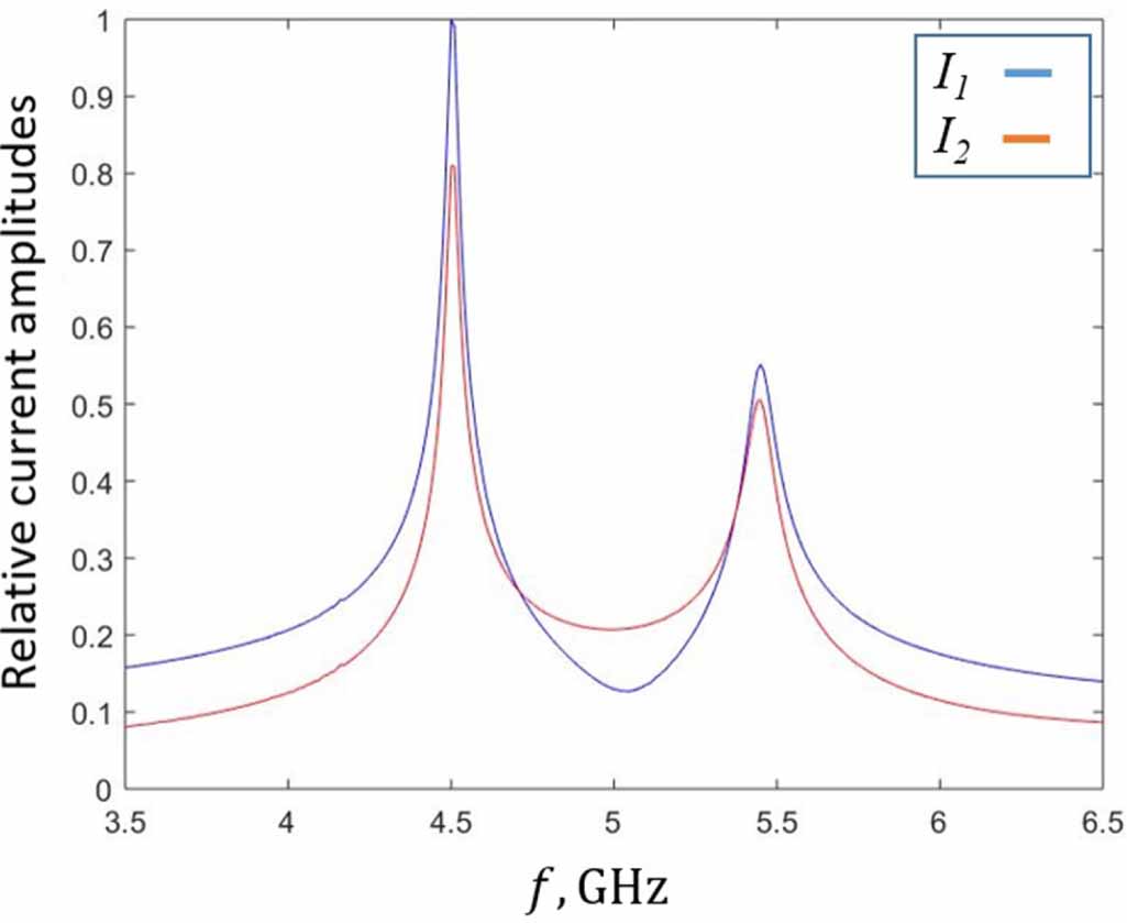
To illustrate the influence of the sign of the coupling coefficients, an example of analytically calculated currents is shown on figure 2. Normalised frequency dependence of the current amplitude for the case of one element is shown in figure 2(a). In figures 2(b) and (c) there are normalised frequency dependencies of the current amplitudes and phase difference between these currents for 2 interacting elements with a magnetic coupling coefficient  for b and
  for c. It can be seen that although the splitting of the resonance curve is the same for the same absolute values of coupling, the phase difference between currents in the elements is different. For the positive coupling case the elements are in phase at the lower frequency resonance and in antiphase at the higher frequency resonance. However for negative coupling the currents for the lower frequency resonance are in antiphase, while for the higher frequency one they are in phase.
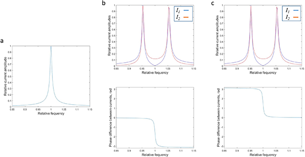
Figure 2. (a) Analytic frequency dependence for current amplitude in a single resonating element. (b) Analytic frequency dependence for current amplitudes and phase differences between them for two coupled element with a magnetic coupling coefficient κ = 0.2. (c) Analytic frequency dependence for current amplitudes and phase differences between them for two coupled element with a magnetic coupling coefficient  .
.
Download figure:
Standard image High-resolution imageTo retrieve the values of both magnetic and electric coupling coefficients separately from measurement or simulation data, a coupling retrieval method has been proposed by one of the current authors in a previous work [23] and then improved upon for the dense metamaterial case in [24]. The retrieval procedure is based on the analysis of equation (5). The coupling coefficient on the right-hand side of (5) can be seen to have two contributions, a magnetic term which is independent of frequency, and an electric term which will vary linearly with the parameter  . It is possible to evaluate both of these components by taking a least squares linear fit (with
  and
and  used as the fit parameters) of the left hand side of equation (5). This data is obtained using a frequency dependent ratio of the currents in each element that can be acquired either experimentally or numerically. This method is valid also when there is retardation and the coupling constants are complex; analysing separately the real and the imaginary parts of (5) yields two curves, from which the complex values of couplings can be retrieved. This method allows one to deduce the magnetic and the electric coupling coefficients if the frequency dependence of the currents in both elements are known and only one of the two elements is fed. (Note that both of these requirements may not be true in a particular experimental setup.)
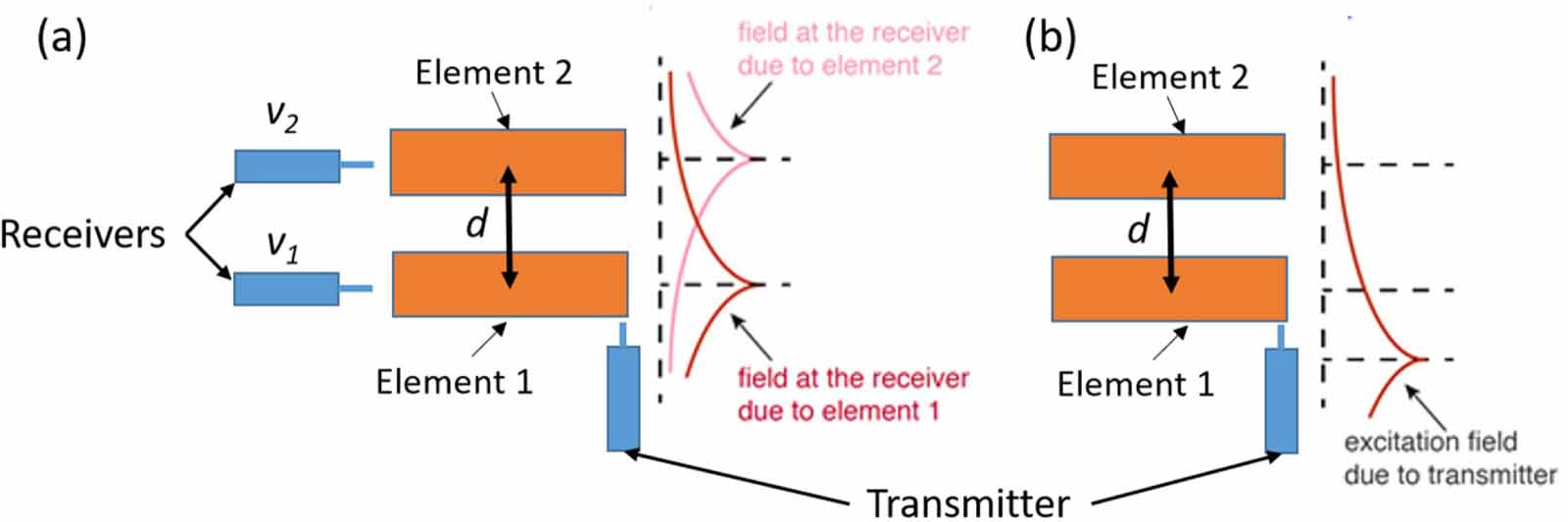
The technique usually employed to determine the currents of two interacting elements 1 and 2, with element 1 being excited, is to place a small exciting (transmitting) antenna close to element 1, and a small receiving antenna next to each of the elements 1 and 2. This can be implemented both in experiment and in COMSOL modelling which will be discussed in the following section. However for the closely packed structure studied in [24], the voltage induced in the receiver will capture the superposition of the fields produced by the current of the primary element and, to a smaller extent, by the neighbouring element as well, as illustrated in figure 3(a). Moreover the influence of the second element may be different for the data measured next to elements 1 and 2 due to the possible asymmetry of their geometry. In addition there is a weak contribution arising directly from the transmitter. However, as the receiver is commonly positioned on the far side of the element away from the feeding probe, which itself is very sub-wavelength, the signal from it at the point of measurement is two orders of magnitude smaller than the one from either of the elements at their resonance frequencies. Further this weak direct signal from the exciting probe can be estimated and easily subtracted from the measurements and all further discussion will assume that subtraction of this direct transmitted signal is already completed.

Figure 3. (a) Overlapping coefficient accounts for a stray field induced by the current in element 1 while measuring the field of the current in element 2 and vice versa. (b) Parasitic excitation coefficient accounts for a weak direct excitation field from a small transmitter placed next to element 1 affecting directly element 2.
Download figure:
Standard image High-resolution imageTo take the influence of the other element into account it is necessary to introduce overlap coefficients α1 for the second element contribution to the measurement recorded in the receiver at element 1 and α2 for the first element contribution to the measurement at element 2. The relationship between measured voltages v1 and v2 and the currents I1 and I2 may thus be written as,

The corresponding ratio of currents that are used in the equation (5) may be written as,
Also, in case of a densely packed structure, the transmitter will excite not only element 1 but, to a smaller extent, also element 2, as illustrated in figure 3(b). Introducing a correction factor to account for this parasitic excitation  , results in equations (1) and (2) changing to


 is a mutual inductance between elements. Now, expressing I1 from equation (10), substituting it to equation (11) and solving it for I2 we obtain:
The ratio of currents in this case can be written as:
that can be finally rearranged in the form of equation (5).
By taking into account both of these correction factors we obtain a method for determining separately the magnetic and the electric coupling coefficients in a densely packed metamaterial. It is valid for metamaterial elements of different shapes and resonant frequencies as the only crucial limitation is for meta-atoms and their spacing to be much smaller than the operating wavelength.
3. Numerical modelling method
In this section, an overview of the numerical method that is used to complement the experimental work presented is discussed. The finite element method (FEM) is implemented using the frequency domain solver of the commercially available package COMSOL Multiphysics (Licence number - 7075 265).
Maxwell's equations are solved over the spherical volume with  and
and  and with a radius that equates to
  at the resonant frequency of the helices. The examined structure consists of two identical copper helices and a small electric probe feeding the first one. The exciting probe is significantly sub-wavelength and operates away from its resonance. Thus it is very weakly coupled to the elements in order to avoid it causing a significant shift in the resonant frequency of the first helix. The probe is driven by a lumped port. It defines the oscillating voltage in the probe with 1 V amplitude over the set frequency range. The overall model volume is limited by a perfectly matched layer (PML) to absorb the excited mode from the source port [25]. Impedance boundary conditions are used for all conductive boundaries in the model.
An example of modelled helices geometry is demonstrated on figure 4, where number of turns n = 4.5, length l = 3 mm, outer radius R = 1 mm, and the wire width w = 0.2 mm. The distance between helix centres is d = 2.4 mm (0.4 mm between edges).
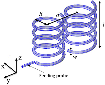
Figure 4. Geometry of the COMSOL model for the two right handed helix structures having the following parameters: number of turns n = 4.5, length l = 3 mm, radius R = 1 mm, wire diameter w = 0.2 mm. The distance between helix centres is d = 2.4 mm.
Download figure:
Standard image High-resolution imageDue to the skin effect, the current at the studied frequencies would propagate, in pure copper, within a skin layer of around 1 micrometer thickness. However there is a surface roughness of order 6 micrometers [26]. Thus the effective copper conductivity is much reduced. The value for this effective conductivity was established by matching the quality factor of the single helix obtained from the experiment to the numerical model. This resulted in an effective resistivity of  .
.
The frequency dependence of the electric current densities I1 and I2 are obtained at the surface of the third turn of each helix using the point evaluation tool in COMSOL. This allows us to avoid the signal overlapping problem, however the parasitic excitation can not be found directly, as it is impossible to prevent the field from the transmitter interacting directly with the second element. However it is still possible to estimate its value. As the frequency dependence of currents in the resonant elements is not proportional to the frequency dependence of the feeding voltage, and it is not possible to calculate the feed of the second helix exactly, the calculation of β was based on the value of currents away from resonance where the currents can be assumed to behave proportionally to the feeding voltage. Taking this into account, the overlapping coefficient can be found as a ratio of current density measured in the second element in the absence of the first one to the current density in the first element alone as in figures 5(b) and (a) respectively. However, this estimate ( ) will be different to the actual value of parasitic excitation.
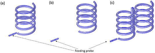
Figure 5. Geometry of the structures used to define the parasitic correction factor β: (a) second element is removed; (b) first element is removed; (c) first element is shorted.
Download figure:
Standard image High-resolution imageIn the case of two helices there are two sources of charges in the first one. First, they are excited due to the induced feeding voltage, resulting in a charge distribution associated with the resonance of the helix and this governs the electric coupling. However as the feeding in the studied case is not direct the feeding probe creates an external field, which induces electrostatic charge on the subwavelength metallic helix. This electrostatic charge also contributes to parasitic excitation and has to be taken into account. Thus to find another estimate of β we short the first helix using a conductive rod connecting all turns of the helix (figure 5), and  can be obtained by finding the ratio of the current density in this case to the one from figure 5(a). The electrostatic contribution in this case can is expected to be stronger than for the initial case due to the larger metallic surface of the shorted helix. As a result, as an estimate for the coupling retrieval method one can use the mean value of
  and
and  . The systematic error associated with this value will be the dominant source of uncertainty for the described model. A way to estimate the resulting uncertainty in coupling values will be discussed in the next subsection.
3.1. Coupling retrieval for numerical data
As an example of the application of the coupling retrieval method to numerical data we shall analyse the simple structure shown in figure 6. This structure consists of two right-handed helices with the parameters given in the previous section. The lowest resonant frequency of each helix is f0 = 5.1 GHz and the quality factor is Q = 58. In the following sections we will label such structures 'normal' as the line connecting the helices centres is orthogonal to the helices axes. Here the start and the end point of the helices are oriented in such a way that the electric dipole moments e1 and e2 are parallel to each other and lie in the yz plane as demonstrated in figure 6. As the electric dipoles here are not in line with the magnetic ones (because of the non-integer number of turns), the axial orientation of each of the helices will have a significant influence on their coupling, which will be further described in the following sections.

Figure 6. Geometry of the COMSOL model for the two right handed helix structures with the schematic representation of electric e1 and magnetic m1 dipole moments orientation at the lowest resonance of the structure.
Download figure:
Standard image High-resolution imageThe frequency dependence of the relative current densities (I1 and I2) presented in figure 7 have been obtained as discussed in the previous section. The phase difference  between them is shown in figure 8.
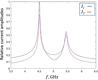
Figure 7. Numerical (FEM) results for frequency dependence of the current density amplitudes for two interacting helices. Distance between the helices is d = 2.4 mm.
Download figure:
Standard image High-resolution image
Figure 8. Numerical results for the frequency dependence of the phase difference between current densities in two interacting helices. Distance between the helices is d = 2.4 mm.
Download figure:
Standard image High-resolution imageBefore applying the retrieval method to this data, the parasitic excitation coefficient β = 0.17 has been obtained as described above. Now by applying the formula (16) to these data the following dependencies of  over ν2 can be obtained for both real, figure 9 and imaginary, figure 10 parts of the coupling coefficients. The red line shows a linear fit to the model data. As is expected, the behaviour is primarily linear. The peaks near the resonant frequencies correspond to the fact that the exciting probe couples to the first element and shifts its resonant frequency slightly. Thus the near zero condition of
  shifts relative to the one of
  resulting in the non linear behaviour of equation (16) near the resonance. In cases where the feeding system affects the resonance significantly, an effective ω0 can be used as the frequency where the zero condition of
  is satisfied. The weak curvature at higher frequencies is related to retardation effects. Estimated random uncertainties are obtained using the standard deviation method and are about 0.5
 .
.

Figure 9. Blue line corresponds to the real part of the numerically obtained dependence of  against ν2 for the currents shown in figures 7 and 8. Red line is a linear fit.
Download figure:
Standard image High-resolution image
Figure 10. Blue line corresponds to the imaginary part of the numerically obtained dependence of  against ν2 for the currents shown in figures 7 and 8. Red line is a linear fit.
Download figure:
Standard image High-resolution imageNow, using the linear fit across the whole frequency range we obtain the coupling coefficients as  and
and  . It can be seen that both magnetic and electric coupling are negative, and retardation (imaginary part) is negligible because of the small size of the structure
  .
.
In order to validate the method and to estimate the uncertainty, the same approach has been applied to model data obtained for the same pair of helices but fed with the probe oriented along different directions. The results were obtained for the probe lying along the x-axis and the z-axis as well as ones at 45 degrees to each axis. In these geometries the coupling between elements stays the same, while the parasitic excitation changes significantly. The mean values of the coupling coefficients obtained for those geometries are  and
and  with uncertainties of
  and
and  , which are mainly connected to the systematic error in β evaluation.
4. Experimental setup
In this section the experimental arrangement used to obtain the coupling data from the helix structures discussed in the previous sections is described. Copper helices with the same parameters as used for modelling have been manufactured by Huidong Linglong Spring Co. A photograph of two right handed helices is shown in figure 11(a). The experimental setup is schematically shown in figure 11(b). Two electric field probes were used. For this purpose we have used a stripped coaxial cable with outer radius of 1 mm, inner wire radius 0.1 mm with a stripped part length of 2 mm. The first probe is used for excitation, while the second is a receiver to measure values of v1 and v2, used in combination with a 40 GHz Vector Network Analyzer (Anritsu MS4644A). Positioning of the probes was controlled to a precision of 0.1 mm using a computer controlled XYZ-translation stage, and the helices were arranged manually so that the end of each helix was positioned close to the corresponding probe (figure 11(a)). The end and start points of the helices are positioned the same way as in the numerical model (figure 4).

Figure 11. (a) Photograph of the experimental arrangement for the two helix coupling retrieval measurement. (b) Schematic representation of the general experimental arrangement for coupling retrieval measurements.
Download figure:
Standard image High-resolution imageTo calculate the overlap coefficient a similar arrangement was used, but with only the first element present. Two measurements are taken, one  with the probe just next to the first helix, and then
  at the place where the second element should be. The overlap coefficient can than be estimated as
  . The same measurement was done for α2, but the fed element was now treated as the second one, and
  was measured at the place where the 1st element would be. We are using the value of the overlap coefficient averaged across the frequency range in order to avoid additional sources of noise in the resulting current data. This noise can be taken into account as the statistical error in the value of the overlap coefficient.
The parasitic excitation has been estimated using the same arrangement as used for the COMSOL data (figures 5(a) and (b)) as the frequency averaged ratio of the signal measured from the second element in the absence of the first one to  . Here we not only take into account the statistical error but also assume a level of systematic uncertainty at the same level as obtained in the numerical modelling.
4.1. Coupling retrieval for the experimental data
Values for currents in each element were obtained as discussed in previous sections and the frequency dependence for the current amplitudes are shown in figure 12 and their phase differences in figure 13. A series of five field measurements described in section 4 have been done, and the averaged value of phase difference between currents have been taken. Statistical uncertainty is marked in grey. Overlapping coefficients used are  and
and  and the parasitic excitation is
  . The resulting currents and the phase difference between them are in a good agreement with the COMSOL model results.

Figure 12. Frequency dependence of the normalised current amplitudes in two interacting helices obtained using corresponding experimental signals. Distance between helix centres is d = 2.4 mm.
Download figure:
Standard image High-resolution image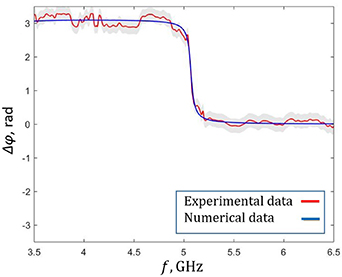
Figure 13. Frequency dependence of the phase difference between currents in two interacting helices obtained from corresponding experimental signals. Distance between helix centres is d = 2.4 mm. Shaded area corresponds to the statistical error.
Download figure:
Standard image High-resolution imageBy using the same method as for the numerical data, the experimental dependencies of  as a function of ν2 are obtained for both the real and imaginary parts of the coupling: see figures 14 and 15 respectively. Again the averaged values of coupling have been taken and statistical uncertainty calculated. Grey shaded area corresponds to the statistical error. It can be seen that the least uncertain values are observed near the resonance of the structure, where the noise to signal ratio is low. However the majority of the data is measured away from the resonance where signal values are low and the noise to signal ratio is high that is further accentuated due to dividing one of the weak signals by the other. Now, again taking a linear fit across the whole frequency range we obtain the following values of coupling coefficients:
  and
and  with uncertainties of
  and
and  . The uncertainties are found based on the systematic and statistical uncertainties discussed above and the standard deviation. These results agree to within the experimental uncertainty with the numerical ones.

Figure 14. Blue dots correspond to the real part of the experimental dependence of  on ν2 for the currents shown in figures 12 and 13. Red line is the linear fit. Shaded area corresponds to the statistical error. Black dashed lines indicate the resonance frequencies of the pair.
Download figure:
Standard image High-resolution image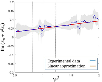
Figure 15. Blue dots correspond to the imaginary part of the experimental dependence of  on ν2 for the currents shown in figures 12 and 13. Red line is the linear fit. Shaded area corresponds to the statistical error. Black dashed lines indicate the resonance frequencies of the pair.
Download figure:
Standard image High-resolution image5. Influence of the mutual arrangement of the helices
5.1. Normal configuration
As stated in previous sections, coupling between helices is strongly anisotropic. Thus, to be able to construct complex metamaterial structures it is important to study different orientations of the helical elements. To begin with we consider the structure of closely arranged 4.5-turn copper helices that were discussed in previous sections (l = 3 mm, R = 1 mm, f0 = 5.1 GHz and Q = 58). As has been shown before, the electric and magnetic coupling coefficients for the normal configuration with 2.4 mm centre to centre distance are both negative and the magnetic one is dominant. First we consider rotation of the second element around its own axis with the first one being fixed. The angle dependencies for the real values of both  and
and  are shown on figure 16(a), and an illustration of the element's arrangements are presented on figures 16(b) and (c) respectively. As has been shown before, the imaginary parts of coupling are small for such sub-wavelength structures and may be neglected for such closely arranged elements. Thus only the real parts of coupling will be examined in this section. To show the effect of the systematic uncertainty discussed in the previous sections, coupling values corresponding to both high and low estimates of parasitic excitations are presented. As the value of β does not change with the rotation of the second helix, the uncertainty limits are the same for all the points on the graph. It can be seen that both couplings are negative at all rotation angles. The relative change of the strength of the magnetic coupling with rotation angle is small compared to the change of the electric contribution. This is because the charge density of the lowest order mode of the helix is concentrated at the ends of the element, thus the optimal way to induce charges in the second element is to arrange one of its ends close to one of the ends of the first element. This is a strong perturbation with rotation angle compared to that associated with the inhomogeneous distribution of currents giving a small variation for the magnetic coupling. Experimental values of couplings obtained for this configuration
  and
and  are in good agreement with numerical ones.

Figure 16. (a) Numerical results for the dependence of the electric and magnetic coupling coefficients on the axial rotation angle of the second element in the normal configuration. (b) and (c) COMSOL models for 0 and 180 degrees rotation respectively.
Download figure:
Standard image High-resolution image5.2. Axial configuration
Now we move to the 'axial' configuration when the axes of the helices are arranged on the same line and explore the same rotation of the second element as for the previous geometry. We consider the same helices as before with a 0.4 mm gap between ends (d = 3.4 mm). The angle dependencies for the real values of both  and
and  are shown in figure 17(a), and illustrations of the element's arrangement are demonstrated in figures 16(b) and (c) respectively. Again, the coupling values corresponding to both high and low estimates of parasitic excitation are presented.
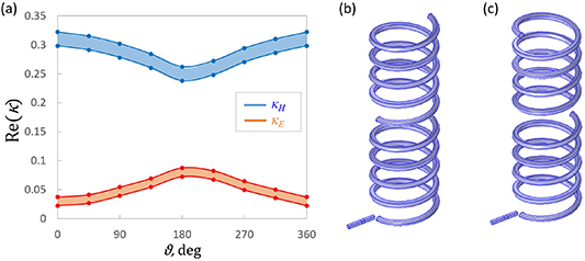
Figure 17. (a) Numerical results for the dependence of the electric and magnetic coupling coefficients on the axial rotation angle of the second element in axial configuration. (b) and (c) COMSOL models for 0 and 180 degrees rotation respectively.
Download figure:
Standard image High-resolution imageIn this configuration couplings are now both positive as the electric and magnetic dipoles of the first element support the same orientation dipoles in the second one. The value of  has again only minor dependence on the rotation angle, while the electric one changes dramatically due to the same reasons as for the normal arrangement. Experimental results for 0 degree rotation are,
  and
and  , and for the 180 one,
  and
and  . The relatively weak
  compared to the normal arrangement case corresponds to the fact that only one end of the first element's effective electric dipole is close to the second element, while the other end of the dipole is shielded by both helices.
5.3. Zero configuration
In the above sections we have found that couplings for the normal arrangement are both negative, and in the axial arrangement, they are both positive, so it is interesting to consider a possible geometry that provides zero value of total coupling. Previous published work has shown that a zero coupling condition can be obtained for split ring resonators [27]. For the helices zero coupling can be obtained in the following way: we start with the normal structure and shift the second helix vertically along its axis. At some point, that is strongly dependent on the geometry of the helices, we will find a position which gives no splitting of the resonance curve. The FEM model of this point for our helices is shown in figure 18 with a spacing along the x axis of 0.4 mm and a Z axis shift of 2.1 mm that is 62 of the helix length. At this position the coupling values for these helices are
  and
and  . Total coupling in this configuration is zero with equal magnitude positive magnetic and negative electric components. Relatively high uncertainties arise from the estimation of the parasitic excitation, which does not scale down since the value of β stays at the level of 0.2.
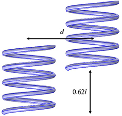
Figure 18. Geometry of the two element structure with zero total coupling.
Download figure:
Standard image High-resolution imageConfiguration of helices similar to the ones discussed in this section have been already implemented in various metamaterial arrays [14–16]. However, the knowledge of coupling between nearest elements, obtained using the discussed retrieval method, allows one to further optimise the metamaterial performance and even construct arrays with predefined dispersion properties. For instance, the analytical approach that connects the dispersion properties of metamaterial to the magnetic coupling coefficients between individual elements can be found in [3, 4, 7]. Based on this, the correct coupling coefficients are chosen for the desired performance, and then the presented coupling retrieval method is used to find the element configuration with the particular coupling. In the following sections we will discuss the behaviour of coupling values in several particular situations and point out their possible practical applications. In the following sections we will discuss the behaviour of coupling values in several particular situations and point out their possible practical applications.
6. Magnetic and electric coupling dependence on the distance between helices
This section is dedicated to experimental and numerical results for the dependence on the distance between them of the coupling coefficients of two helices for both normal and axial configurations. We will consider structures formed from the two helices discussed in the previous sections and vary their centre to centre distance d. Numerical and experimental results of  and
and  dependence on d are presented on figures 19 and 20 for normal and axial configurations respectively. Uncertainties in the experimental results are marked with error bars and the statistical error in the numerical ones is indicated by the coupling values corresponding to both high and low estimates of parasitic excitation. It is important to notice that as the distance between elements grows, the feeding probe excites the second element much less and the parasitic excitation coefficient becomes smaller and the width between the two uncertainty bounds diminishes accordingly.
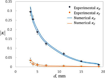
Figure 19. Numerical and experimental results for the electric and magnetic coupling dependence on the distance between helices in the normal configuration.
Download figure:
Standard image High-resolution image
Figure 20. Numerical and experimental results for the electric and magnetic coupling dependence on the distance between helices in the axial configuration.
Download figure:
Standard image High-resolution imageExperimental results appear to be in good agreement with numerical ones for all distances and both geometries. As may be expected both electric and magnetic couplings weaken with d. In order to compare this data with analytical equations (6) and (7) it is useful to rearrange the data for the magnetic coupling into a log-log plot as shown on figure 21. It can be seen that the slopes for both normal and axial configurations are of order −1.2 that corresponds to  dependence suggested by the analytical calculations, which predicts a slope of −1. The difference is readily explained by the fact that helices are not point dipoles and
  at small distances.
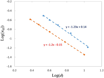
Figure 21. Numerical and experimental results for the absolute values of electric and magnetic coupling dependence on the distance between helices in normal (red) and axial (blue) configurations.
Download figure:
Standard image High-resolution imageThe coupling dependence on the distance between elements, while being helpful in the design of metamaterial arrays, may be particularly useful for the metamaterial inspired applications such as miniature superdirective antennas, where both the spacing and the coupling strength have to be tuned in order to obtain close to theoretical maximum antenna performance. The general approach to the design and characterisation of such structures is found in [20].
7. Different handed helices
In previous sections we have studied couplings between two right handed helices. Identical results, except for the axial rotation when equivalent angles are of opposite sign, can be obtained for two left handed ones. However the combination of right and left handed helices provides a very different response. In figure 22 one can see the geometries and corresponding coupling values for both a normal and axial pair formed from one right handed and one left handed 4.5-turn helix. It can be seen that magnetic couplings in this case have the same sign and approximately the same amplitude as for the same handed case. However the sign of the electric coupling has changed. This happens because magnetic coupling is the dominant contribution in this structure, so the current in the second element flows in the opposite direction compared to the first one. Thus, for the left handed helix, in normal configurations, the negative magnetic coupling results in the opposite direction of current flow which induces electric charges with the same vertical distribution as in the first one. As a result the charge distribution at the second element corresponds to positive electric coupling. Moreover as  and
and  counteract each other the total coupling strength for the different handed helices is much smaller then for the same handed ones. Distribution of charges and currents for this case is schematically shown in figure 23.
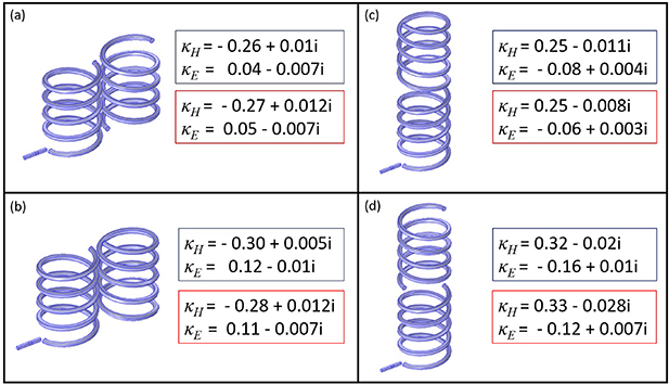
Figure 22. Normal ((a) and (b)) and axial ((c) and (d)) geometries of pairs of right and left handed 4.5-turn helices with 0 and 180 degrees rotation of the second element respectively, with the corresponding numerical (blue) and experimental (red) results for the electric and magnetic coupling coefficients.
Download figure:
Standard image High-resolution image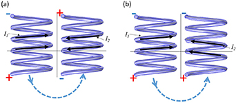
Figure 23. Schematic representation of the charges and currents distributions for the same (a) and the opposite (b) handed helices.
Download figure:
Standard image High-resolution imageThe use of helices with different handedness provides greater control over coupling values for a set distance between elements that may be used in cases where an exact value of coupling is required to obtain the theoretical maximum performance, for instance, the design of artificial magnetic conductors [21]. The analytical approach that may be used to find the coupling coefficients required for a particular AMC response is found in [28]. In addition to this, knowledge of particular coupling values may be used to optimise the response of structures where different handed helices are used to provide metamaterial absorbers [15, 17, 18] or polarization converters [19].
8. Geometric parameters influence on coupling
8.1. Number of turns
In previous sections we have considered only helices with 4.5 turns. To illustrate how electric coupling is affected by the distribution of charge densities we will now examine the case of 5-turn right handed helices with all other parameters staying the same. The resonant frequency of such helices is f0 = 5 GHz. Numerical results for normal and axial configurations of such helices are shown on figure 24. It can be seen that for the axial configuration the relative charge distributions have stayed the same and thus the coupling values are at the same level. However for the normal one, when charges are in the closest arrangement figure 24(b), an electric coupling of −0.16 is found, that is much stronger than the maximum value for the 4.5-turn case (−0.11). On the other hand, when both elements are 180 degrees rotated figure 24(a), and so quite far apart, the electric coupling is decreased to  . The magnitude of the magnetic coupling in these cases are similar to that of the 4.5-turn case, as current distributions stay almost the same.

Figure 24. Normal ((a) and (b)) and axial ((c) and (d)) geometries of pairs of 5-turn helices with 0 and 180 degrees rotation of the second element respectively, with the corresponding numerical (blue) and experimental (red) results for the electric and magnetic coupling coefficients.
Download figure:
Standard image High-resolution image8.2. Axial pitch
We now consider changing the axial pitch of the helices, by stretching them in the axial direction. Both numerical and experimental results for normal and axial configurations of 5-turn helices with l = 11 mm are presented in figure 25. The other parameters of the helices are still the same as before. The electric coupling in this case has a similar magnitude compared to previous cases and follows the same pattern: the stronger electric coupling is observed when the electric charge concentrations are closer to each other. However, as the magnetic flux produced by more sparsely arranged loops is no longer so well confined within the helix an overlap of magnetic fields can be observed not only between helices as a whole but also between the individual loops. This leads to stronger magnetic coupling in the normal arrangement compared to l = 3 mm case. On the other hand, the z component of the magnetic flux at the top and bottom of the helices becomes smaller and thus, weaker magnetic coupling is obtained in the axial configuration.
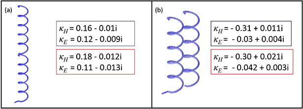
Figure 25. Normal (a) and axial (b) geometries of pairs of 5-turn stretched helices, with the corresponding numerical (blue) and experimental (red) results for the electric and magnetic coupling coefficients.
Download figure:
Standard image High-resolution imageIf the axial pitch is smaller with the total height of the helix being 1.2 mm, as shown in figure 26, the effect is of course the opposite. The magnetic field here is more solenoid-like, thus less magnetic flux overlaps with the neighboring helix in the normal arrangement reducing the negative magnetic coupling in case (a). On the other hand the positive coupling in the axial configuration becomes even stronger.
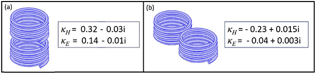
Figure 26. Normal (a) and axial (b) geometries of pairs of 5-turn shrunk helices, with the corresponding numerical (blue) and experimental (red) results for the electric and magnetic coupling coefficients.
Download figure:
Standard image High-resolution image8.3. Capped helices
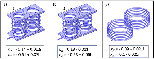
In the previous sections magnetic coupling has been dominant between helical elements. Here we will examine elements that have a dominant electric coupling component. To design such elements we add metallic caps (cap size A = 2.2 mm) to the top and bottom of the 5-turn helices considered in the first subsection of this section. Holes with radius  = 0.9 mm are left in the center of the caps to reduce magnetic shielding by the caps. The resonance frequency of this structure is reduced to 3.9 GHz due to the higher self capacitance of the elements. In figure 27 coupling coefficients are shown for capped helices with the same (a) and different (b) handedness in the normal configuration. Electric coupling here is dominant, at the level of
  , while the magnetic coupling is smaller than in the previous cases due to the partial magnetic field shielding by the metallic caps. Hence, the charge and current distributions are governed by electric coupling, so in the case of different handed helices, the magnetic coupling changes sign.
Figure 27. Geometries and corresponding numerical results for the electric and magnetic coupling coefficients for the normal arrangement pairs of 5-turn capped helices: (a) same handed helices; (b) different handed helices; (c) different handed helices with total coupling tending to 0.
Download figure:
Standard image High-resolution image
This provides an alternate route to obtain a geometry with zero total coupling. First, in order to reduce electric coupling, one may replace the caps at the ends of the helices with flat round discs. Secondly, to strengthen magnetic coupling, the inner radius of the hole in the discs should be increased. Then for a structure with helix radius R = 4 mm, hole radius  = 3.8 mm, and cap radius
  = 4.2 mm it is possible to obtain zero coupling with opposite handed helices,
  and
and  when the distance between centers is a = 5 mm. The geometry is illustrated on figure 27. Such structures may be implemented for elaborate metamaterial devices where careful control of collective effects between meta-atoms is required. The coupling coefficients between helices can be adjusted for the particular applications depending on the performance requirements. For instance superdirective antennas can benefit from elements with low quality factor [20]; a small number of turns is necessary for artificial magnetic conductor structures [21]; while large negative values of coupling provided by capped helices allows one to design broadband surfaces with negative mode index [22]. Finally the mutual orientation of electric and magnetic dipoles in helices is important for the polarisation control of radiated signal in antenna applications as well as for the passive structures used for the polarisation conversion.
9. Conclusions
In this work the coupling retrieval method has been implemented to obtain numerical and experimental values for both electric and magnetic coupling coefficients between helical elements. First we explored the interaction between pairs of identical half-integer turn right (or left) handed copper helices and then opposite handed helices in both normal and axial configurations. It has been shown that for such elements magnetic coupling is dominant and the sign of both electric and magnetic couplings depends on the mutual arrangement of elements. The use of the different handed helices gives an opportunity to explore structures in which electric and magnetic couplings have different signs. The influence of axial rotation of helices on  and
and  as well as the dependence of couplings on the distance between element centres has been studied. The effects of the number of turns and the axial pitch has been explored and a way to produce a structure of capped helices with dominant electric coupling has been modelled. Furthermore, the geometries with both negative and positive
  and
and  as well as all their possible combinations have been demonstrated including the two geometries where the electric and magnetic coupling have the same amplitude and opposite sign so that the total coupling is zero so there is no splitting of the resonance curve.
Results of this work can be used to construct metamaterials with predefined properties including broadband metasurfaces with negative mode index, sub-wavelength superdirective antenna arrays and artificial magnetic conductors. For these and other possible metamaterial structures the coupling coefficients between helical elements will be used to meet the analytical conditions and maximise the performance of the structure.
Acknowledgments
We acknowledge financial support from the Engineering and Physical Sciences Research Council (EPSRC) of the United Kingdom via the EPSRC Centre for Doctoral Training in Metamaterials (Grant No. EP/L015331/1). We also acknowledge financial support from the Defence Science and Technology Laboratory (Dstl) (Contract No. DSTLX1000133579).
Data availability statement
The data that support the findings of this study are available upon reasonable request from the authors.