

Abstract
We study a heavy–heavy–light three-body system confined to one space dimension in the regime where an excited state in the heavy–light subsystems becomes weakly bound. The associated two-body system is characterized by (i) the structure of the weakly-bound excited heavy–light state and (ii) the presence of deeply-bound heavy–light states. The consequences of these aspects for the behavior of the three-body system are analyzed. We find a strong indication for universal behavior of both three-body binding energies and wave functions for different weakly-bound excited states in the heavy–light subsystems.
Export citation and abstract BibTeX RIS

Original content from this work may be used under the terms of the Creative Commons Attribution 4.0 licence. Any further distribution of this work must maintain attribution to the author(s) and the title of the work, journal citation and DOI.
1. Introduction
Already relatively simple few-body systems, like a configuration of three pairwise interacting identical bosons in three dimensions, display rich features as the Efimov effect [1, 2]. This is the emergence of an infinite sequence of universal three-body bound states provided there are at least two s-wave resonant pair-interactions. Here, universality means that the three-body states are independent of the details of the two-body interaction [3, 4]. The Efimov effect is enhanced in a two-component three-body system with a large mass ratio between the two species [5–7]. The existence of these Efimov states is strongly restricted to particular values of the total angular momentum [8, 9], the dimension of space [10–12], and the symmetry of the weakly-bound (or virtual) two-body state [13–15], including combinations thereof. Changing any of these system properties may prohibit the Efimov effect, however, there can still be universal three-body bound states [9, 11, 14, 16].
Recently, we have proven universality [17, 18] in a heavy–heavy–light three-body system, which is confined to one dimension (1D). The universality requires the heavy–light interactions to be tuned towards the ground-state threshold, that is the binding energy of the ground state approaches zero. Indeed, in this limit, the three-body binding energies and wave functions for arbitrary short-range two-body interactions converge to the respective ones found for the zero-range interaction.
In this article we study the universality of the same three-body system provided the heavy–light interactions are tuned towards an excited-state threshold, that is the binding energy of an excited state approaches zero. This situation occurs in most experiments employing ultracold atoms. In comparison to the case of the ground-state threshold, this implies (i) that the weakly-bound heavy–light state can either be symmetric or antisymmetric and (ii) the presence of deeply-bound heavy–light states. We analyze such three-body systems by solving the Faddeev equations numerically for different finite-range potentials. We identify the same universal behavior for three-body binding energies, regardless of whether the threshold is characterized by a symmetric or antisymmetric weakly-bound heavy–light state. In contrast, we demonstrate that the universal limit of the corresponding three-body wave functions is distinct for these two different symmetries. Moreover, within the separable approximation [19–21] of the finite-range interactions, we find that the deeply-bound heavy–light states play a crucial role in the universal limit. The three-body bound states presented in this article belong to the class of so-called bound states in a continuum [22–24].
Our research supports the increasing interest in few- and many-body systems confined to low dimensions. Already many decades ago, the Tonks–Girardeau gas [25, 26] and the Lieb–Liniger model [27, 28] have been considered, which are based on the zero-range contact interaction [29]. Three-body systems in 1D have recently [30–32] attracted increasing attention. In particular, studies on the inclusion of three-body interactions [33–35], on three-body systems of two different species [17, 36], and on the accuracy of adiabatic methods [17, 37] have been performed.
Not only theoretical studies but also experimental measurements of few-body effects in low dimensions are nowadays feasible. For this purpose, ultracold gases are confined via anisotropic traps leading to cigar- or tube-shaped configurations [38, 39]. Moreover, the strength of interactions in ultracold gases can be tuned over the scope of many orders of magnitude with the help of Feshbach resonances [40] or so-called confinement-induced resonances [41, 42]. Experimental observations of few-body effects have been brought to an entirely new level of detail by manipulating ultracold atoms on the single-atom scale [43, 44], ensuring pure few-body effects.
Most theoretical studies [17, 34–37, 45, 46] of three-body systems confined along two directions are based on 1D models. This complexity reduction offers the advantage of a simple and intuitive description revealing the underlying three-body properties. However, it is important to keep in mind that experiments employing these confined systems are always performed in quasi-1D. The conditions to reproduce the results predicted by a pure 2D model in a quasi-2D experiment and accordingly by a 1D model in a quasi-1D setup have been discussed in references [47–49].
Our article is organized as follows. In section 2 we introduce the class of three-body systems, which is the focus of our study and precisely formulate our goals. We present in section 3 the corresponding energies and wave functions of three-body bound states in the system. In particular, we analyze the universal behavior of these quantities close to different energy thresholds of the two-body system. Next, we discuss in section 4 the influence of deeply-bound two-body states on the universal behavior of the three-body system. Finally, we conclude by summarizing our results and presenting an outlook in section 5. To keep our article self-contained, but focused on the central ideas we collect in appendix
2. The three-body system
In this section we first introduce a one-dimensional two-body system governed by a pair interaction. Next, by adding a third particle we arrive at the class of three-body systems, which is the focus of this article. We then present characteristic quantities of the three-body system, which are central to our subsequent studies. Finally, we describe the analytical and numerical methods employed to determine the three-body binding energies and wave functions.
2.1. Two interacting particles
We consider a two-body system consisting of a heavy particle of mass M and a light one of mass m, both constrained to 1D and interacting via a potential of finite range ξ0. We define the mass ratio α ≡ M/m of the two particles in the heavy–light system.
After eliminating the heavy–light center-of-mass coordinate, the system is governed by the stationary Schrödinger equation

for the two-body wave function  of the relative motion presented in dimensionless units. Here, ξ denotes the relative coordinate of the light particle with respect to the heavy one in units of the characteristic length ξ0.
The two-body binding energy  and the potential

are both given in units of  with the Planck constant ℏ and the reduced mass μ ≡ M/(1 + α) of the heavy–light system. Here, v0 denotes the magnitude and f the shape of the interaction potential.
We assume an attractive interaction with v0 < 0 and ∫dξf(ξ) > 0, as well as a symmetric shape f, that is  . Moreover, we choose v such that it describes a short-range interaction, i.e.
  as
as  .
.
In particular, we perform the analysis in this article for different two-body interactions of finite-range, namely a potential having the polynomially decaying shape

of the cube of a Lorentzian, and one with the shape

of a Gaussian decaying exponentially.
In contrast to the zero-range interaction of shape

the finite-range potentials whose shapes are determined by equations (3) and (4) can support more than a single bound state, depending on the magnitude v0.
We label the two-body wave function  and the binding energy
  as solutions of equation (1) by the index r, where r = 0, 1, 2, ... denotes the number of nodes of
  . Even values of r indicate symmetric two-body wave functions, whereas odd values indicate antisymmetric ones, that is

2.2. Three interacting particles
We now add a third particle to the two-body system, also constrained to 1D and identical to the other heavy particle of mass M. We assume the same interaction between each heavy and the light particle as introduced in section 2.1, but no interaction between the two heavy ones. The resulting three-body system is depicted in figure 1. Here, y23 denotes the relative coordinate between the two heavy particles (called here particles 2 and 3) and x1 the relative coordinate of the light particle (particle 1) with respect to the center of mass C of the two heavy ones, both in units of the characteristic length ξ0.

Figure 1. Jacobi-coordinates x1 and y23 for the three-body system consisting of one light particle of mass m (blue) and two heavy ones of mass M (red), all confined to 1D. Here, C denotes the center of mass of the two heavy particles.
Download figure:
Standard image High-resolution imageBy eliminating the center-of-mass motion of this heavy–heavy–light system, we arrive at the Schrödinger equation
for the three-body wave function  of the two relative motions in coordinate representation. The coefficients αx
≡ (1 + 2α)/[2(1 + α)] and αy
≡ 2/(1 + α) depend only on the mass ratio α, and
of the two relative motions in coordinate representation. The coefficients αx
≡ (1 + 2α)/[2(1 + α)] and αy
≡ 2/(1 + α) depend only on the mass ratio α, and  is the dimensionless three-body energy in units of
  .
.
2.3. Formulation of the problem
In this article, we determine the energies and wave functions of bound states in the three-body system, provided the heavy–light subsystems support a weakly-bound excited state, that is  for r = 1, 2, 3. We are mainly interested in the question of whether or not there exist three-body quantities that show universal behavior in these cases. Universality denotes the property of physical quantities to show a behavior that is independent of the short-range details of the interparticle interactions.
In reference [17], we have studied the situation when the heavy–light system is tuned to the ground-state threshold (r = 0). We have found universality in terms of both energies and corresponding wave functions of three-body bound states for  . In this limit, we have proven that for arbitrary attractive short-range heavy–light interactions obeying the conditions in section 2.1, the three-body energies and wave functions converge to the respective ones induced by a heavy–light contact interaction of shape fδ
, equation (5).
. In this limit, we have proven that for arbitrary attractive short-range heavy–light interactions obeying the conditions in section 2.1, the three-body energies and wave functions converge to the respective ones induced by a heavy–light contact interaction of shape fδ
, equation (5).
The differences between the ground- and an excited-state threshold are as follows. Tuning the heavy–light subsystems to an excited-state energy threshold immediately implies (i) a different number r of nodes and therefore a possibly different symmetry of the corresponding weakly-bound two-body bound state, and (ii) the existence of deeply-bound two-body states, whose binding energy does not approach zero. Depending on the symmetry of the weakly-bound two-body wave function, equation (6), we speak of even-numbered (r = 0, 2, ...) and odd-numbered (r = 1, 3, ...) thresholds.
We analyze the effect of both features on the universal behavior of energies and wave functions of three-body bound states close to an excited-state threshold in the heavy–light subsystems. We emphasize that there are two kinds of three-body bound states, namely (i) excited three-body bound states associated with the respective threshold, and (ii) deeply-lying three-body bound states. (i) The excited three-body bound states are embedded in a continuum that originates from deeply-bound heavy–light states in combination with an unbound heavy particle. For these states we expect a universal behavior. (ii) The deeply-bound three-body states keep a finite size when the excited-state threshold is approached, hence we expect them to be sensitive to the details of the interaction. For this reason, they do not show universal behavior and we refrain from analyzing them in this article.
The excited three-body states are so-called bound states in the continuum [24]. These states have a real-valued energy, but are positioned in the continuum of scattering states, that is  . Bound states in the continuum have been predicted [22, 23, 50] and realized [51–54] in a variety of physical systems. There are several mechanisms that can protect these states against decay into the continuum states, e.g. modulation of the interaction potential [22, 23], interference of resonances [50] and symmetry protection [51, 52]. For example the latter might be of relevance in our three-body system, as depending on the threshold r, the three-body bound states display a different symmetry than the continuum in which it is embedded. Nevertheless, we want to emphasize that in the current article the focus lies on obtaining such bound states in the continuum, and most importantly in analyzing their universality. We therefore refrain here from a deeper investigation of the underlying mechanism that allows their existence.
Apart from bound states, we want to mention that there can further exist three-body resonances [55–57] that are also located above the lowest two-body energy threshold, . These resonances are however characterized by a non-vanishing imaginary part
  of the three-body energy and are not studied in the present article.
Similar to the results [17] found near the ground-state threshold  , we expect a set of universal three-body bound states associated with each heavy–light threshold
  characterized by the index r. To distinguish between these sets, we introduce the notation
  for the energy of the nth three-body bound state |ψr,n
⟩ within the rth set. As shown in the following, we indicate with even and odd values of n the case of the two heavy particles being bosons or fermions, respectively.
for the energy of the nth three-body bound state |ψr,n
⟩ within the rth set. As shown in the following, we indicate with even and odd values of n the case of the two heavy particles being bosons or fermions, respectively.
In order to reveal the dependency of three-body universality on (i) the symmetry of the weakly-bound state and (ii) the existence of deeply-bound states in the heavy–light subsystems, we compare the energies and wave functions of three-body bound states for r > 0 with the corresponding ones for r = 0. Due to the reported [17] universality for r = 0, we can use the scale-invariant three-body binding energies and wave functions for the heavy–light contact interaction as representatives for this set of states. We therefore base our analysis on the following two quantities:
(a) The relative deviation

between the energy ratios  r,n
and
r,n
and  . Here,

denotes the ratio of the nth three-body bound state energy  within the rth set to the energy
  of the weakly-bound heavy–light bound state. Moreover, we define the ratio

between the corresponding three- and two-body energies found for the special case of a contact heavy–light interaction of shape fδ , equation (5).
(b) The fidelity

defined as the overlap between a three-body bound-state |ψr,n
⟩ for a finite-range heavy–light potential, and the corresponding state  for the contact interaction in arbitrary representation.
2.4. Methods
We solve equation (7) within the framework of the Faddeev equations [20, 58]. There we can easily incorporate the necessary boundary condition

to obtain three-body bound states embedded in a continuum. For this reason, we consider the homogeneous form of the Faddeev equations. In order to select other types of states, e.g. resonance or scattering states, a different form of the boundary condition and therefore of the Faddeev equations is required. However, in this article, we restrict ourselves to bound states in the continuum which obey equation (12).
We show in appendix
of the Faddeev component ϕ(2) evaluated at different arguments. Here, k23 denotes the relative momentum between particles 2 and 3, whereas p1 is the momentum of particle 1 relative to the center of mass of particles 2 and 3.
Moreover, the plus and minus signs in equation (13) distinguish the case of the two heavy particles being bosons or fermions. This is evident from considering the exchange of the two heavy particles being described by k23 → −k23 which leads to the exchange symmetry

for the total three-body wave function. As k23 is the momentum corresponding to the relative distance y23 between the two heavy particles, the symmetry (antisymmetry) of ψ(k23, p1) with respect to the line k23 = 0 directly relates via the Fourier transform to the symmetry (antisymmetry) of the wave function ψ(y23, x1) with respect to the line y23 = 0 in coordinate space.
The separable expansion [19–21] simplifies the Faddeev equations (see appendix

in terms of products of functions depending on only one momentum variable. Here,  and the functions gν
and τν
≡ −ην
/(1 − ην
) are determined by the eigenvalue equation
and the functions gν
and τν
≡ −ην
/(1 − ην
) are determined by the eigenvalue equation

where

is the momentum representation of the heavy–light potential v(ξ), equation (2).
For a given r > 0 and ν ⩽ r the functions gν
can be related to the wave functions  of the two-body bound states, however with variable energy argument
  . Indeed, for a given v0, they are connected to each other only when
  [19, 20]. The term with ν = r describes the one close to the threshold and the terms with ν < r correspond to the deeply-bound heavy–light states. We can reveal the influence of the latter for the prediction of the correct three-body universality by excluding single terms with ν < r in the expansion, equation (15), and comparing the subsequent results to the ones without excluding them. This is performed in section 4.
For the functions φν
we derive in appendix
which yields the same energy solutions  as the Schrödinger equation (7).
As mentioned above, we consider in this article three-body bound states with the boundary conditions, equation (12), embedded in a continuum associated with deeply-bound heavy–light states together with an unbound heavy particle. They therefore correspond to real energy solutions  . The three-body bound state energy
  enters the kernels in equation (18) as a parameter, hence the solutions
  are obtained by varying over a suitable region
 and requiring eigenvalue unity (minus unity) for bosons (fermions). The functions φν
are obtained as the corresponding eigenvectors.
and requiring eigenvalue unity (minus unity) for bosons (fermions). The functions φν
are obtained as the corresponding eigenvectors.
Equation (18) is a system of coupled homogeneous Fredholm integral equations of the second kind. We solve it numerically by truncating the infinite number of expansion terms in equations (15) and (18) to a finite value νmax, and approximating the continuous interval for p and q by a discrete grid. This reduces equation (18) to a finite system of coupled matrix eigenvalue problems. In our analysis νmax = 10 has yielded sufficient convergence.
3. Results
In this section we present the energies and wave functions of three-body bound states associated with the two-body threshold  for r = 1,r = 2 and r = 3. For this purpose, we have solved equation (18) numerically for two finite-range interaction potentials of shape fL, equation (3), and fG, equation (4). By varying the magnitude v0 of the potential, we can tune the heavy–light subsystems to a particular threshold.
The mass ratio between heavy and light particles directly influences the number of three-body bound states [17, 36]. In the following we choose a mass ratio of α = M/m = 20 for which there is a total of six three-body bound states associated to the ground-state heavy–light threshold, three each for the case of bosonic and fermionic heavy particles. In the next subsections we show that the number of respective three-body bound states in one set remains the same near an excited-state heavy–light threshold.
The ratios  , equation (10), obtained for a contact heavy–light interaction and the mass ratio M/m = 20 are listed in table 1. Due to the scale-invariant nature of the delta-potential, they are independent of the heavy–light binding energy. Since all three-body binding energies associated with a weakly-bound heavy–light state lie below the corresponding two-body threshold, all ratios are smaller than −1.
Table 1. Energy ratios  , equation (10), for the two-body contact interaction fδ
, equation (5), and the mass ratio M/m = 20. As shown in reference [17], they represent the universal limits obtained for attractive short-range heavy–light interactions in the case
, equation (10), for the two-body contact interaction fδ
, equation (5), and the mass ratio M/m = 20. As shown in reference [17], they represent the universal limits obtained for attractive short-range heavy–light interactions in the case  .
.
| n | Bosons | Fermions |
|---|---|---|
| 0 | −2.7238 | — |
| 1 | — | −1.6517 |
| 2 | −1.3285 | — |
| 3 | — | −1.1240 |
| 4 | −1.0373 | — |
| 5 | — | −1.0004 |
3.1. Energy spectrum
We start by analyzing the universality in the energy spectrum of the three-body system. In figure 2 we present the relative deviation Δr,n
, equation (8), between the energy ratio r,n
, equation (9), obtained in the case of a finite-range heavy–light interaction and the energy ratio  , equation (10), for a zero-range heavy–light interaction, equation (5), as a function of the two-body binding energy
  . Throughout the subfigures we indicate by filled red and empty blue symbols the results for an interaction of shape fL, equation (3), and fG, equation (4), respectively. The top row shows Δ1,n
near the first excited heavy–light threshold,
. Throughout the subfigures we indicate by filled red and empty blue symbols the results for an interaction of shape fL, equation (3), and fG, equation (4), respectively. The top row shows Δ1,n
near the first excited heavy–light threshold,  , the central row Δ2,n
for
, the central row Δ2,n
for  , and the bottom row Δ3,n
for the third excited state,
, and the bottom row Δ3,n
for the third excited state,  . The left and right columns display the case of two heavy bosons (n = 0, 2, 4) or fermions (n = 1, 3, 5), respectively.
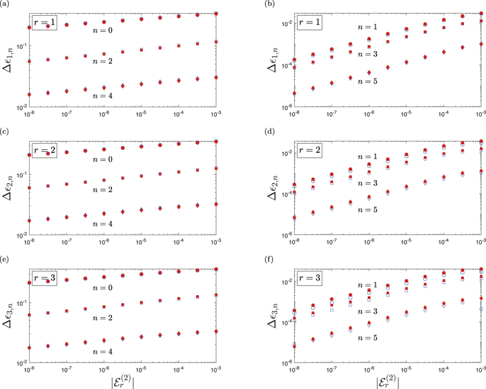
Figure 2. Relative deviation Δr,n
, equation (8), of the energy ratio r,n
, equation (9), from the energy ratio  , equation (10), as a function of the two-body binding energy
  . Here we present the results for the excited-state thresholds with r = 1 (top row), r = 2 (center row), and r = 3, (bottom row). The left and right columns distinguish between the case of two heavy bosons and two heavy fermions. The results are shown for finite-range potentials of shape fL, equation (3), (filled red symbols) and fG, equation (4), (empty blue symbols). For a mass ratio of M/m = 20 there are six three-body bound states associated to the individual heavy–light thresholds, three each for the case of bosons or fermions.
Download figure:
Standard image High-resolution imageFor all three thresholds (r = 1, 2, 3) and all three-body bound states (n = 0, ..., 5), the filled red and empty blue data sets are very close to each other. We highlight that this is true throughout the entire range of two-body energies displayed here. Moreover, the deviation between the red and blue data sets is decreasing as the threshold is approached. Thus, universality is indicated by the fact that near each threshold, the same energy ratios are achieved for the different finite-range interactions.
Next, we compare the universal behavior near the different heavy–light thresholds. For all considered cases r = 1, 2, 3, the relative deviations Δr,n
are decreasing strictly monotonically towards zero as  . Hence, the energy ratios r,n
associated to all three excited-state two-body thresholds converge towards the same limit values
. Hence, the energy ratios r,n
associated to all three excited-state two-body thresholds converge towards the same limit values  , table 1, as for the ground-state threshold. This explicitly implies that the universal limits of the three-body energies are identical for symmetric (r = 0, 2, ...) and antisymmetric (r = 1, 3, ...) weakly-bound states in the heavy–light subsystems. Moreover, we observe that for each three-body state labeled by n, the results for the considered thresholds r = 1, 2, 3 behave almost identical throughout the entire range of two-body binding energies.
In particular, the deviations Δr,n
appear to decrease as a power law, as indicated by the linear dependence in the double-logarithmic scale. The corresponding slopes, which in return denote the exponent of the power law, are listed in table 2 and have been obtained via linear regression and for the potential of Gaussian shape fG, equation (4). The slopes for r > 0 are smaller compared to those for r = 0. This relates to a slower convergence towards the universal three-body energies near excited-state thresholds compared to the ground-state one. The difference between the thresholds r = 0 and r > 0 is characterized by the presence of deeply-bound states in the latter cases. Hence these deeply-bound states have a crucial influence on how fast the universal limit is approached. Moreover, for each respective state labeled by n, we observe that the slopes are almost identical for all r > 0. We note that Δr,n
, equation (8), is defined as an absolute value, hence our analysis does not distinguish whether the limit values  are approached from above or below.
Table 2. Exponents of the suggested power law behavior of Δr,n
, equation (8), corresponding to the slopes of the linear dependence in the double-logarithmic scale, figure 2. These values have been obtained via a linear regression for the potential of Gaussian shape fG, equation (4). The corresponding results for r = 0 are analyzed in more detail in reference [17] and not shown explicitly in figure 2.
| r | n | Bosons | n | Fermions |
|---|---|---|---|---|
| 0 | 0 | 0.992 | 1 | 0.986 |
| 2 | 1.087 | 3 | 0.991 | |
| 4 | 1.000 | 5 | 0.989 | |
| 1 | 0 | 0.046 | 1 | 0.461 |
| 2 | 0.065 | 3 | 0.463 | |
| 4 | 0.057 | 5 | 0.488 | |
| 2 | 0 | 0.046 | 1 | 0.475 |
| 2 | 0.067 | 3 | 0.475 | |
| 4 | 0.057 | 5 | 0.468 | |
| 3 | 0 | 0.046 | 1 | 0.469 |
| 2 | 0.067 | 3 | 0.469 | |
| 4 | 0.056 | 5 | 0.485 |
We can further analyze the universal behavior for different excited three-body states characterized by the index n. In the case of fermions (odd n) the relative deviation of r,n
from  is much smaller and decreases much faster than in the case of bosons (even n) when approaching the threshold, as indicated by the different range of the vertical axes. Indeed, this is also reflected in the values of the corresponding slopes, table 2, which are almost a factor of ten larger for fermions compared to bosons. This striking difference in the universal behavior is a pure three-body effect due to the fact that the property of the two heavy particles being bosons or fermions does not change the heavy–light two-body problem. Finally, we observe a smaller deviation Δr,n
for states with larger index n.
is much smaller and decreases much faster than in the case of bosons (even n) when approaching the threshold, as indicated by the different range of the vertical axes. Indeed, this is also reflected in the values of the corresponding slopes, table 2, which are almost a factor of ten larger for fermions compared to bosons. This striking difference in the universal behavior is a pure three-body effect due to the fact that the property of the two heavy particles being bosons or fermions does not change the heavy–light two-body problem. Finally, we observe a smaller deviation Δr,n
for states with larger index n.
3.2. Wave functions
Having found that the universal limit of the three-body binding energies is the same when even-numbered and odd-numbered thresholds are approached, we now turn to the analysis in terms of the corresponding three-body wave functions. Since the wave functions carry the full information about a quantum state, we aim to obtain a deeper insight into three-body universality from their study.
For this purpose, we compare the three-body wave functions for the two finite-range potentials of shape fL, equation (3), and fG, equation (4), tuned near the excited-state thresholds r = 1, 2, 3, to the ones resulting from a contact heavy–light interaction with fδ
, equation (5), by means of the fidelity Fr,n
defined by equation (11). As previously mentioned we use the results for the contact interaction as scale-invariant representatives for the case r = 0. Moreover, in order to compare the universal behavior for weakly-bound excited heavy–light states of the same symmetry, we consider the overlap  of the three-body wave functions for the two odd-numbered thresholds r = 1 and r = 3.
In figure 3 we present the fidelity Fr,n
as a function of the two-body binding energy  . Throughout the subfigures we indicate by filled red and empty blue symbols the fidelities for a heavy–light interaction of shape fL, equation (3), and fG, equation (4), respectively. Analogous to figure 2, the top three rows show the results for three different heavy–light thresholds
  ,
,  and
and  , respectively. In the last row we separately display the overlap |⟨ψ3,n
|ψ1,n
⟩|2. The left and right columns distinguish the case of two heavy bosons (n = 0, 2, 4) or fermions (n = 1, 3, 5), respectively.
, respectively. In the last row we separately display the overlap |⟨ψ3,n
|ψ1,n
⟩|2. The left and right columns distinguish the case of two heavy bosons (n = 0, 2, 4) or fermions (n = 1, 3, 5), respectively.
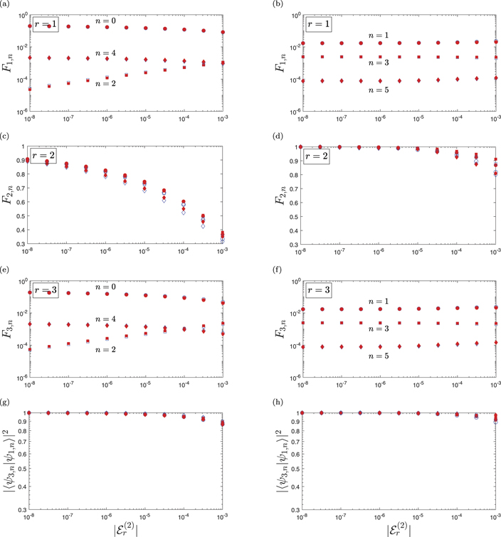
Figure 3. Fidelity Fr,n
, equation (11), as a function of the two-body binding energy  . We focus here on the excited-state thresholds r = 1 (top row), r = 2 (center-top row) and r = 3 (center-bottom row). Moreover, we display the overlap |⟨ψ3,n
|ψ1,n
⟩|2 (bottom row) between the three-body wave functions associated with the odd-numbered thresholds r = 1 and r = 3. The left and right columns distinguish between the case of two heavy bosons and two heavy fermions. The fidelities are presented for finite-range potentials of shape fL, equation (3) (filled red symbols) and fG, equation (4) (empty blue symbols). For a mass ratio of M/m = 20 there are six three-body bound states associated to the individual heavy–light thresholds, three each for the case of bosons or fermions.
. We focus here on the excited-state thresholds r = 1 (top row), r = 2 (center-top row) and r = 3 (center-bottom row). Moreover, we display the overlap |⟨ψ3,n
|ψ1,n
⟩|2 (bottom row) between the three-body wave functions associated with the odd-numbered thresholds r = 1 and r = 3. The left and right columns distinguish between the case of two heavy bosons and two heavy fermions. The fidelities are presented for finite-range potentials of shape fL, equation (3) (filled red symbols) and fG, equation (4) (empty blue symbols). For a mass ratio of M/m = 20 there are six three-body bound states associated to the individual heavy–light thresholds, three each for the case of bosons or fermions.
Download figure:
Standard image High-resolution imageA comparison of the fidelities between the two different finite-range heavy–light interactions shows a similar behavior as for the three-body energies. In all subfigures the corresponding red and blue data sets are very close to each other and thus suggest the universality of the wave functions of three-body bound states.
Next, we analyze the universal behavior of the fidelities for different weakly-bound states in the heavy–light subsystems. In contrast to the results for the energies, which show the same universal limit for all values of r, we observe that the fidelities near the three excited-state thresholds display a fundamentally different behavior. A fidelity of unity indicates that the two wave functions overlap perfectly and are therefore identical. On the other hand a vanishing fidelity indicates that the two wave functions ψr,n
and  are orthogonal. For the even-numbered threshold (r = 2) the fidelities F2,n
are increasing and approaching unity as the threshold is approached, as demonstrated in figures 3(c) and (d). Contrarily, for the odd-numbered thresholds (r = 1 and r = 3) the fidelities F1,n
and F3,n
are far below unity, as evident from figures 3(a), (b), (e) and (f). However, the overlap |⟨ψ3,n
|ψ1,n
⟩|2 between the three-body wave functions near the odd-numbered thresholds approaches again unity as
are orthogonal. For the even-numbered threshold (r = 2) the fidelities F2,n
are increasing and approaching unity as the threshold is approached, as demonstrated in figures 3(c) and (d). Contrarily, for the odd-numbered thresholds (r = 1 and r = 3) the fidelities F1,n
and F3,n
are far below unity, as evident from figures 3(a), (b), (e) and (f). However, the overlap |⟨ψ3,n
|ψ1,n
⟩|2 between the three-body wave functions near the odd-numbered thresholds approaches again unity as  , see figures 3(g) and (h).
To conclude, these results for the fidelities indicate that the three-body wave functions approach two distinct universal limits, one for symmetric, and another one for antisymmetric weakly-bound heavy–light states. The universal limits for the symmetric case are those for the zero-range contact interaction. On the other hand, the universal limits for the antisymmetric case might correspond to those obtained for an odd-wave pseudopotential [29]. We recall that such a dependence on the symmetry of the weakly-bound heavy–light state has not become apparent in the universal limit of the respective three-body energies.
Finally, we analyze the universal behavior for different excited three-body states characterized by the index n. Near the even-numbered threshold (r = 2), the fidelities F2,n
are larger for fermionic heavy particles (odd n) than for bosonic ones (even n) and the limit value for  is reached faster. This is in accordance with the results for the energies shown in figure 2. In contrast, near the odd-numbered thresholds (r = 1 and r = 3) the overlap |⟨ψ3,n
|ψ1,n
⟩|2 shows no significant difference between bosons and fermions. The fidelities F1,n
and F3,n
are far below unity and therefore we refrain from analyzing them in more detail.
is reached faster. This is in accordance with the results for the energies shown in figure 2. In contrast, near the odd-numbered thresholds (r = 1 and r = 3) the overlap |⟨ψ3,n
|ψ1,n
⟩|2 shows no significant difference between bosons and fermions. The fidelities F1,n
and F3,n
are far below unity and therefore we refrain from analyzing them in more detail.
In order to reinforce our results, we display contour plots of the wave functions in figure 4. We restrict ourselves here to the potential shape fG, equation (4), of the heavy–light interaction and to the most deeply-bound states for the case of bosons(n = 0) and fermions (n = 1). The wave functions are displayed in momentum space

scaled by the two-body energy  of the corresponding weakly-bound heavy–light state.
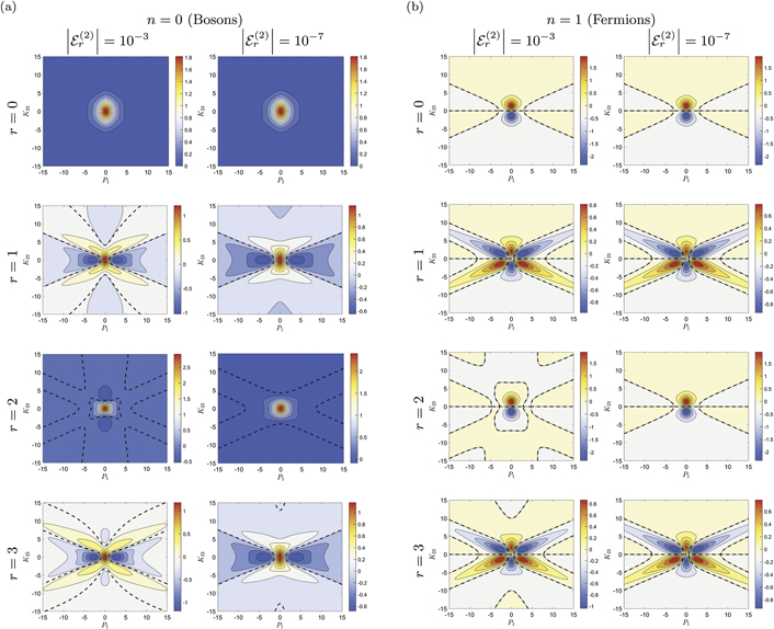
Figure 4. Contour plots of the normalized three-body wave functions ψr,n
(K23, P1) in the space spanned by the scaled momenta, equation (19), as obtained for the heavy–light interaction of shape fG, equation (4). The rows distinguish between the different two-body thresholds, r = 0 (top), r = 1 (center-top), r = 2 (center-bottom) and r = 3 (bottom). The diagrams are split into two halves, corresponding to (a) bosons (n = 0) and (b) fermions (n = 1). Each half is split again into two columns, the left column in each half shows the case of  , and the right column the case of
  . The contours where the wave functions vanish are highlighted by dashed black lines.
Download figure:
Standard image High-resolution imageThe four rows distinguish the two-body thresholds r = 0 (top), r = 1 (center-top), r = 2 (center-bottom) and r = 3 (bottom). The diagrams are split into two halves, the left one (a) corresponds to bosons (n = 0) whereas the right one (b) corresponds to fermions (n = 1). Each half is split again into two columns, the left column in each half displays the wave functions for the two-body binding energy  , and the right column for
  . The contours of zero value for the wave functions are highlighted by black dashed lines.
First we discuss the even-numbered thresholds. The three-body wave functions near the ground state threshold r = 0 (top) and the excited-state threshold r = 2 (center-bottom) look already very similar for the respective state n. This similarity is further enhanced when the two-body threshold is approached. This behavior is in line with the fidelities increasing towards unity as presented in figures 3(c) and (d). Hence, from this we deduce that the three-body wave functions for the even-numbered heavy–light thresholds approach the same universal limit.
Next, we consider the odd-numbered thresholds. As presented in figure 4, the three-body wave functions forr = 1 (center-top) and r = 3 (bottom) are very similar, but look fundamentally different from those obtained near the even-numbered thresholds r = 0 (top) and r = 2 (center-bottom). This is in agreement with the high overlap shown in figures 3(g) and (h) and the low values of the corresponding fidelities (figures 3(a), (b), (e) and (f)). As a result, this expresses that the same universal limit of the three-body wave functions is approached near all odd-numbered heavy–light thresholds. However, this limit is distinct from the limit near even-numbered thresholds.
Subsequently, we analyze the three-body wave functions depending on the index n in order to highlight differences and similarities between the cases of two heavy bosons (n = 0) and fermions (n = 1). This property of the two heavy particles can be identified for all values of r from the symmetry with respect to the line K23 = 0, as evident from figure 4 and summarized by equation (14). As pointed out already in section 2.4, this statement translates in coordinate space to the same symmetry with respect to the exchange y23 → −y23. As an example, the three-body wave functions in coordinate representation are displayed in reference [17] for the contact interaction (r = 0). However, already from figure 4 it is apparent that the bosonic wave functions have parity +1, whereas the fermionic ones have parity −1, which is summarized by equation (14).
For these two different kinds of heavy particles, we now discuss the speed of convergence towards a scale-invariant three-body bound state when a particular two-body threshold is approached. With scale-invariance we mean here that the wave functions expressed in the scaled momenta, equation (19), behave like a constant as a function of  . Near the ground-state threshold (r = 0) both bosonic (figure 4(a)) and fermionic (figure 4(b)) wave functions look identical for the presented two-body binding energies
  and
and  . This is because they have already reached the scale-invariant limit [17]. However, for the excited-state thresholds (r > 0), the structure of the bosonic wave functions (figure 4(a)) still changes quite significantly when decreasing the two-body binding energy. On the other hand, the fermionic wave functions (figure 4(b)) are already much closer to the scale-invariant regime. This behavior of the wave functions also enables a better understanding of the results presented in figure 3. Indeed, the fidelities for r = 2 are lower for bosons, figure 3(c), than for fermions, figure 3(d). Consequently, we observe a major difference between bosons and fermions in their speed of convergence towards the scale-invariant regime. This is in line with the results for the energy spectrum, discussed in subsection 3.1. In conclusion, we note that the difference in the wave functions having an extremum (bosons, figure 4(a)) or zero (fermions, figure 4(b)) at the line K23 = 0 might explain this faster convergence of the energies and wave functions for the fermionic case in comparison to the bosonic one.
Finally, we address another aspect of the universal behavior of the three-body bound states. Indeed, in each column of figure 4, that is for fixed two-body binding energies  , the wave functions for both bosons and fermions associated with the odd-numbered thresholds (r = 1 and r = 3) look very similar. We point out that this is true although the bosonic ones have not yet reached the scale-invariant regime. This also explains why the overlap |⟨ψ3,n
|ψ1,n
⟩|2 between the three-body wave functions near odd-numbered thresholds does not display a significant difference as shown in figure 3(g) for the bosonic, and in figure 3(h) for the fermionic case. We expect the same behavior when comparing the results for any two excited-state thresholds for which the associated weakly-bound states have the same symmetry, i.e. r = 2 and r = 4.
, the wave functions for both bosons and fermions associated with the odd-numbered thresholds (r = 1 and r = 3) look very similar. We point out that this is true although the bosonic ones have not yet reached the scale-invariant regime. This also explains why the overlap |⟨ψ3,n
|ψ1,n
⟩|2 between the three-body wave functions near odd-numbered thresholds does not display a significant difference as shown in figure 3(g) for the bosonic, and in figure 3(h) for the fermionic case. We expect the same behavior when comparing the results for any two excited-state thresholds for which the associated weakly-bound states have the same symmetry, i.e. r = 2 and r = 4.
4. Influence of deeply-bound two-body states on the three-body universality
In the preceding section we have found universality in the three-body system, when the heavy–light subsystems are tuned towards an excited-state threshold. In particular, the universality of the three-body wave functions depends on the symmetry of the weakly-bound state in the heavy–light subsystems. A natural question therefore arises whether the universal behavior is solely determined by this weakly-bound state.
In order to answer this question we analyze in this section the influence of deeply-bound heavy–light states on the universal limit in the three-body system. These deeply-bound states have a nonzero binding energy and are naturally implied when the heavy–light subsystems are tuned close to an excited-state threshold. We focus our attention here on the energy ratios r,n
, equation (9).
The separable expansion [19, 20], outlined in appendix  , each term in equation (15) with ν ⩽ r is related to a deeply-bound state in the heavy–light subsystem, provided the energy arguments
  coincide with the energy
  of the respective two-body state. Similarly, for
  , the term ν = r describes the weakly-bound two-body bound state. Thus, the influence of the deeply-bound two-body states on the universality of three-body bound states associated to a particular threshold (r > 0) can be tested by manually including and excluding different terms with ν < r.
Here we consider as an example the case r = 2 where there are two (ν = 0 and ν = 1) deeply-bound states in the heavy–light system in addition to the weakly-bound state with ν = 2. Moreover, the fermionic case (n = 1) is chosen because of its faster convergence in the limit of vanishing two-body binding energy  compared to the bosonic case. In figure 5 we illustrate the influence of the deeply-bound states on the energy ratio
  . This ratio converges towards r,n
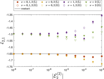
, equation (9), provided that all expansion terms are included in equations (15) and (18). To explore the influence of particular expansion terms on the three-body energy, we consider different combinations in the expansion as indicated by the legend. Filled symbols mark the results for an interaction potential of shape fL, equation (3), and empty ones for the shape fG, equation (4). We consider four different combinations:
. This ratio converges towards r,n
, equation (9), provided that all expansion terms are included in equations (15) and (18). To explore the influence of particular expansion terms on the three-body energy, we consider different combinations in the expansion as indicated by the legend. Filled symbols mark the results for an interaction potential of shape fL, equation (3), and empty ones for the shape fG, equation (4). We consider four different combinations:
- (a)(ν = 0, 1, 2; red dots) if both deeply-bound two-body states and the weakly-bound one are included, the ratio
 converges to the limit value for the contact interaction (black line).
 - (b)(ν = 0, 2; yellow squares) excluding the first excited heavy–light bound state (ν = 1) from the analysis has no observable impact on the limit value of the energy ratio.
- (c)(ν = 1, 2; purple diamonds) when excluding instead the heavy–light ground state, described by the term ν = 0, the energy ratio converges to a limit value that is different from of the contact interaction.
- (d)(ν = 2; green triangles) the exclusion of both deeply-bound states with ν = 0 and ν = 1 leads to the same (incorrect) limit value as for (c).


Figure 5. Ratio  of three-body binding energy to
  for r = 2, n = 1 and different numbers of separable terms in equations (15) and (18) as a function of
  . We manually include or exclude different expansion terms as indicated in the legend. Filled symbols display the results for the two-body interaction of shape fL, equation (3), and empty symbols for the shape fG, equation (4), accordingly. The exact result for the energy ratio 2,1 in the limit
  is indicated by a black line.
Download figure:
Standard image High-resolution image
As evident from figure 5 we observe that for all combinations (a)–(d) the limit values for the two finite-rage potentials of shape fL and fG coincide. This interaction-independent behavior is not visibly influenced by the presence or absence of the deeply-bound two-body states. Hence, it is the origin for the universality of the energy ratios r,n
, equation (9), presented in section 3.
On the other hand, the separable approximation, that is taking into account only the term ν = r = 2 corresponding to the weakly-bound state of the heavy–light subsystem, yields a value of  that does not coincide with 2,1. Therefore, the weakly-bound state alone is not sufficient to achieve an agreement with the universal limit for the ground-state two-body threshold. Hence, the result presented in section 3, that the three-body energies approach the same universal limit for all values of r, crucially relies on the presence of the deeply-bound two-body states and cannot be explained by the weakly-bound state ν = r = 2 alone. However, it seems that not all deeply-bound states are equally relevant. For the example presented here, it is the term ν = 0 that is important, whereas the term ν = 1 has a negligible effect on
  in the limit
  .
.
As a result, this analysis indicates that the separable approximation fails in predicting the correct limiting three-body energy ratios, whenever the heavy–light subsystems support deeply-bound two-body states (r > 0). However, in this article we have shown that the correct three-body energy ratios converge to the ones for the contact interaction. Indeed, the universal three-body energies for the finite-range potentials can be obtained when taking into account all deeply-bound states. A similar study on the separable approximation has been performed in reference [21] for three identical bosons in 3D.
5. Conclusion and outlook
In this article we have investigated the universality of a quantum mechanical heavy–heavy–light system constrained to 1D, provided the heavy–light subsystem is tuned to the energy threshold associated with a weakly-bound excited state. In comparison to the case of the ground-state threshold [17], the situation here differs in two main points: (i) the wave function of the weakly-bound heavy–light state has at least one node and its symmetry can change from symmetric to antisymmetric, and (ii) the heavy–light subsystems now contain additional deeply-bound states. We have analyzed the influence of both aspects on the three-body system by solving the Faddeev equations numerically for different finite-range potentials. Moreover, we have compared the resulting energies and wave functions to the corresponding results near the ground-state heavy–light threshold, as represented by those for the contact interaction.
Universality describes the property that a three-body quantity becomes independent of the short-range details of the two-body interaction potential. Since two finite-range potentials with different long-range decay have yielded the same three-body binding energies and wave functions, we have found an indication of universality for these two quantities. In particular, we have demonstrated this behavior near the thresholds corresponding to the first three excited bound states in the heavy–light subsystem. For the ground-state threshold, universality has already been demonstrated and proven in reference [17].
We have further compared the universality of the three-body system for the four heavy–light thresholds characterized by r = 0, 1, 2, 3. For the three-body binding energies, we have observed the same universal limit across all four thresholds. In particular, this suggests that the universal limits of the three-body binding energies do not depend on the symmetry of the weakly-bound heavy–light state. No fundamentally different result is expected near thresholds of higher excited (r > 3) heavy–light states. However, we have found that for r > 0 the speed of convergence towards the universal limit values is slower compared to r = 0. In terms of the corresponding three-body wave functions, we have observed two distinct universal limits, one for all symmetric (r = 0, 2, ...), and a different one for all antisymmetric (r = 1, 3, ...) weakly-bound heavy–light states.
In addition, the universal behavior depends strongly on the property of the two heavy particles being bosons or fermions. In particular, close to an excited-state threshold the three-body energy spectrum and corresponding wave functions in the fermionic case display a scale-invariant behavior at much larger two-body binding energies than in the bosonic one. This is in contrast to the ground-state threshold, where no such difference between bosonic and fermionic heavy particles was observed [17]. We want to highlight here that the characteristics of the two heavy particles being bosons or fermions does not affect the properties of the heavy–light subsystems. Any observed difference in the three-body quantities between the two cases is therefore a pure three-body effect.
Furthermore, we have demonstrated that for finite-range heavy–light interactions tuned close to an excited-state threshold, the separable approximation of the corresponding interactions does not provide the correct universal limits of the three-body energies. As a consequence, the universal limit of the three-body binding energies cannot be explained with the weakly-bound state in the heavy–light subsystems alone. Moreover, we note that an interaction-independent behavior has been observed for all tested combinations of deeply-bound states in the expansion. It appears that not all deeply-bound two-body states are equally important for the universal behavior of the three-body system.
Based on the analysis presented in this article we are convinced that the three-body bound states associated with an excited-state two-body threshold display universality. We want to emphasize that these universal three-body states belong to the class of so-called bound states in the continuum. There are several possible mechanisms that can protect these particular states against decaying into continuum states, e.g. symmetry protection or interference of resonances. Identifying the relevant mechanisms for the investigated three-body system remains however a task for the future.
In order to gain a better understanding of the universal behavior, additional insight into the mechanism of deeply-bound two-body states would be desirable. Another approach would be to apply an adiabatic method as e.g. the Born–Oppenheimer approximation and test whether the three-body universality can be related to a universal Born–Oppenheimer potential. Moreover, it would be interesting to analyze whether an odd-wave pseudopotential [29, 59] can provide the universal limit for the three-body wave functions that we have observed for the odd-numbered thresholds. Such a pseudo-potential could further help in understanding the independence of the universal three-body energies on the symmetry of the weakly-bound heavy–light states. Then, it might be possible to establish a mapping between the results for even and odd-numbered thresholds. Additionally, the striking difference in the convergence speed towards the universal limit between heavy bosons and fermions needs further analysis. Finally, the study of three-body resonances in this one-dimensional system poses an interesting and experimentally relevant task.
Acknowledgments
We are very grateful to P M A Mestrom and W P Schleich for fruitful discussions. LH and MAE thank the Center for Integrated Quantum Science and Technology (IQST) for financial support. The research of the IQST is financially supported by the Ministry of Science, Research and Arts Baden-Württemberg. The authors acknowledge support by the state of Baden-Württemberg through bwHPC and the German Research Foundation (DFG) through Grant No. INST 40/467-1 FUGG (JUSTUS cluster) and INST 40/575-1 FUGG (JUSTUS 2 cluster).
Data availability statement
The data that support the findings of this study are available upon reasonable request from the authors.
Appendix A.: Methods
In this appendix we derive the integral equation, equation (18), corresponding to the three-body Schrödinger equation, equation (7) within the Faddeev approach [20, 58] and the separable expansion [19–21]. We consider the three-body system as introduced in section 2.2, where the light particle of mass m is called particle 1, and particle 2 and 3 are the two identical heavy ones of mass M.
A.1. The Faddeev equations
We start by considering the three-body Schrödinger equation (7) in representation-free form

Here, H0 is the kinetic energy operator without the center-of-mass motion, whereas V31 and V12 describe the pair-interactions between particles 3 and 1, and particles 1 and 2, respectively.
According to the Faddeev approach [20, 58], the solution of the Schrödinger equation (A1) is given by the superposition

of |ϕ(2)⟩ and |ϕ(3)⟩, related to the so-called Faddeev components


Here,  is the three-body Green function corresponding to H0. The Faddeev components obey the Faddeev equations


that is a system of two coupled integral equations.
The matrices T31, T12 are the T-matrices of the three-body system if only the pair-interaction V31 between particle 3 and 1, or V12 between particle 1 and 2 respectively, is present. Hence, T31 and T12 fulfill the Lippmann–Schwinger equation [20]


A.2. Momentum representation
Three-body systems can be described in three different arrangements of relative motions, corresponding to three sets of so-called Jacobi momenta [20]. For {i, j, l} = {1, 2, 3} and the two cyclic permutations thereof we denote by

the relative momentum between the particles i and j, whereas

is the momentum of particle l relative to the center-of-mass of the pair of particles i, j. The momentum and mass of each particle are denoted by ki and mi respectively, with i = 1, 2, 3.
The relations between the Jacobi momenta read


with the mass ratio α = M/m and the coefficients

The system of Faddeev equations (A4a) and (A4b) can be reduced to a single equation using the exchange symmetry between the two identical heavy particles in the three-body system. The exchange of particles 2 and 3 is most easily described in the set of Jacobi momenta k23 and p1 by the transformation k23 → −k23. From equations (A8a)–(A9b) we deduce


We distinguish two cases: the identical particles 2 and 3 are either bosons or fermions. Depending on this property, the total three-body wave function ψ(−k23, p1) = ±ψ(k23, p1) has to preserve (bosons) or flip (fermions) its sign under exchange of the two particles. This fact can be expressed in terms of the Faddeev components via equation (A2) which yields

after the application of  .
.
As a result, we can relate the two Faddeev components to each other


With help of equations (A8a)–(A9b) this allows us to cast the total wave function in the form
Since Φ(3) can be obtained from Φ(2) via equation (A14), it is sufficient to only obtain the Faddeev component Φ(2) from its Faddeev equation (A4a). In momentum representation this equation reads
Using the momentum representation of the free-particle three-body Green function [20, 60]

as well as the relation of the three-body T-matrix to the off-shell two-body t-matrix [20, 60]
allows us to perform the integrations over  ,
,  and
and  in equation (A16). Expressing further via equations (A10a) and (A10b) the momenta −k12 and p3 in terms of k31 and p2 for the arguments of Φ(2)(−k12, p3), we arrive at the integral equation
Here we have omitted the indices of the momenta k31 and p2.
By introducing the change of variables,  , we cast equation (A19) into the form
eliminating the dependence on p in the second argument of Φ(2) inside the integral.
A.3. Separable expansion
We now transform equation (A20) into the form of a Fredholm integral equation of the second kind. For most potentials, the off-shell t-matrix  appearing in equation (A20) cannot be written as a product of functions of k or k' only. However, it is possible to expand the t-matrix into a sum of separable products [19–21]

Here, the functions gν and τν ≡ −ην /(1 − ην ) are determined by the integral equation

with the momentum representation

of the heavy–light potential v(ξ) = v0 f(ξ). The functions gν are orthonormal with respect to the relation

where δν,ν' denotes the Kronecker symbol.
By inserting equation (A21) into (A20), we arrive at the expansion

for Φ(2) with  and
and
Finally, by substituting equation (A25) into (A26), we derive a system of coupled integral equations
in only a single variable for the functions  .
.