Deep null space learning for inverse problems: convergence analysis and rates

Any method for the stable solution of (1.1) uses, either implicitly or explicitly, a priori information about the unknowns to be recovered. Such information can be that $\newcommand{\signal}{x} \signal$ belongs to a certain set of admissible elements $\newcommand{\M}{{\mathcal M}} \M$ or that it has small value of some regularizing functional. The most basic regularization method is probably Tikhonov regularization, where the solution is defined as a minimizer of the quadratic Tikhonov functional

$$\begin{align} \newcommand{\e}{{\rm e}} \newcommand{\tik}{\mathcal{T}} \newcommand{\Ao}{\mathbf A} \newcommand{\data}{y} \newcommand{\signal}{x} \newcommand{\norm}[1]{{\left\Vert#1\right\Vert}} \newcommand{\la}{\lambda} \newcommand{\al}{\alpha} \displaystyle \label{eq:tik} \tik_{\alpha;\data_\delta}(\signal):= \frac{1}{2} \norm{\Ao (\signal) - \data^\delta}^2 + \frac{\alpha}{2} \norm{\signal }^2. \nonumber \end{align} \tag{ 1.2 }$$

Other classical regularization methods for solving linear inverse problems are filter based methods [7], which include Tikhonov regularization as special case.

In the last couple of years variational regularization methods including TV regularization or $\newcommand{\e}{{\rm e}} \ell^q$ regularization became popular [22]. They also include classical Tikhonov regularization as special case. In the general version, the regularizer $\newcommand{\edot}{\,\cdot\,} \newcommand{\norm}[1]{{\left\Vert#1\right\Vert}} \newcommand{\e}{{\rm e}} \frac{1}{2} \norm{\edot }^2$ is replaced by general convex and lower semi-continuous functionals.

In this paper, we develop a new regularization concept that we name $\newcommand{\nun}{\boldsymbol{\Phi}} \nun$-regularization method. Roughly spoken, a $\newcommand{\nun}{\boldsymbol{\Phi}} \nun$-regularization method is a tuple $\newcommand{\R}{{\mathbb R}} \newcommand{\al}{\alpha} \newcommand{\Ro}{\mathbf R} ((\Ro_\al)_{\al >0}, \al^\star)$ where (for a precise definition see definition 2.3)

• $\newcommand{\XX}{X} \newcommand{\M}{{\mathcal M}} \M \subseteq \XX$ is the set of admissible elements, defined by the function Φ;
• $\newcommand{\R}{{\mathbb R}} \newcommand{\al}{\alpha} \newcommand{\XX}{X} \newcommand{\YY}{Y} \newcommand{\Ro}{\mathbf R} \Ro_\al \colon \YY \to \XX$ are continuous mappings;
• $\newcommand{\al}{\alpha} \newcommand{\data}{y} \alpha^\star = \alpha^\star(\delta, \data^\delta)$ is a suitable parameter choice;
• For any $\newcommand{\signal}{x} \newcommand{\M}{{\mathcal M}} \signal \in \M$ we have $\newcommand{\R}{{\mathbb R}} \newcommand{\al}{\alpha} \newcommand{\signal}{x} \newcommand{\data}{y} \newcommand{\Ro}{\mathbf R} \Ro_{\alpha^\star(\delta, \data^\delta)} (\data^\delta) \to \signal$ as $\delta \to 0$.

Note that for some cases is might be reasonable to take $\newcommand{\R}{{\mathbb R}} \newcommand{\al}{\alpha} \newcommand{\Ro}{\mathbf R} \Ro_\al$ multivalued. For the sake of simplicity here we only consider the single-valued case. Classical regularization methods are special cases of $\newcommand{\nun}{\boldsymbol{\Phi}} \nun$-regularization methods in Hilbert spaces where $\newcommand{\Ao}{\mathbf A} \newcommand{\M}{{\mathcal M}} \M = \ker(\Ao)^\bot$. A typical regularization method is in this case given by Tikhonov regularization, where $\newcommand{\R}{{\mathbb R}} \newcommand{\al}{\alpha} \newcommand{\XX}{X} \newcommand{\Ao}{\mathbf A} \newcommand{\Ro}{\mathbf R} \newcommand{\Id}{{\rm Id}} \Ro_\al = (\Ao^* \Ao + \al \Id_{\XX})^{-1} \Ao^*$. Here and in the following $\newcommand{\XX}{X} \newcommand{\Id}{{\rm Id}} \Id_{\XX}$ denotes the identity on $\newcommand{\XX}{X} \XX$.

Very recently, deep learning approaches appeared as alternative, very successful methods for solving inverse problems (see, for example [2–6, 8, 10, 12, 15, 25–28]). In most of these approaches, a reconstruction network $\newcommand{\R}{{\mathbb R}} \newcommand{\XX}{X} \newcommand{\YY}{Y} \newcommand{\Ro}{\mathbf R} \Ro \colon \YY \to \XX$ is trained to map measured data to the desired output image.

Various reconstruction networks have been introduced in the literature. In the two-step approach, the reconstruction networks take the form $\newcommand{\R}{{\mathbb R}} \newcommand{\BP}{\mathbf{B}} \newcommand{\Ro}{\mathbf R} \newcommand{\nsn}{\mathbf{L}} \Ro = \nsn \circ \BP$ where $\newcommand{\XX}{X} \newcommand{\YY}{Y} \newcommand{\BP}{\mathbf{B}} \BP \colon \YY \to \XX$ maps the data to the reconstruction space (reconstruction layer or backprojection; no free parameters) and $\newcommand{\XX}{X} \newcommand{\nsn}{\mathbf{L}} \nsn \colon \XX \to \XX$ is a neural network (NN) whose free parameters are adjusted to the training data. In particular, so called residual networks $\newcommand{\N}{{\mathbb N}} \newcommand{\XX}{X} \newcommand{\Id}{{\rm Id}} \newcommand{\NN}{\mathbf{N}} \newcommand{\nsn}{\mathbf{L}} \nsn = \Id_{\XX} + \NN$ where only the residual part $\newcommand{\N}{{\mathbb N}} \newcommand{\NN}{\mathbf{N}} \NN$ is trained [11] show very accurate results for solving inverse problems [3, 6, 12, 13, 16, 18, 21, 26]. Another class of reconstruction networks learns free parameters in iterative schemes. In such approaches, a sequence of reconstruction networks $\newcommand{\R}{{\mathbb R}} \newcommand{\Ro}{\mathbf R} \Ro = \Ro^{(k)}$ is defined by some iterative process $\newcommand{\R}{{\mathbb R}} \newcommand{\N}{{\mathbb N}} \newcommand{\signal}{x} \newcommand{\data}{y} \newcommand{\Ro}{\mathbf R} \newcommand{\NN}{\mathbf{N}} \Ro^{(k)} (\data) = \NN_k (\Phi_k(\signal_{k-1} , \dots, \signal_{0}, \data))$ where $\newcommand{\signal}{x} \signal_0$ is some the initial guess, $\newcommand{\N}{{\mathbb N}} \newcommand{\XX}{X} \newcommand{\NN}{\mathbf{N}} \NN_k \colon \XX \to \XX$ are networks that can be adjusted to available training data, and $\Phi_k$ are updates based on the data and the previous iterates [2, 14, 15, 23].

Further existing deep learning approaches for solving inverse problems are based on trained projection operators [5, 8], or use neural networks as trained regularization term [17].

While the above deep learning based reconstruction networks empirically yield good performance, none of them is known to be a convergent regularization method. In this paper, we use a new network structure (null space network) that, when combined with a classical regularization of the Moore Penrose inverse is shown to provide a convergent $\newcommand{\nun}{\boldsymbol{\Phi}} \nun$-regularization method with rates. One of the reviewers of this manuscript kindly brought to our attention that the null space network structure actually has been introduced already by Mardani and collaborators in [19, 20] in a finite dimensional setting. We extend the use of the null space network to operators with non-closed range and analyze its stable approximation in the context of regularization methods.

As often argued in the recent literature, deep learning based reconstruction approaches (especially using two-stage networks) lack data consistency, in the sense that outputs of existing reconstruction networks fail to accurately predict the given data. In order to overcome this issue, in this paper, we introduce a new network, that we name null space network. The proposed null space network takes the form

$$\begin{align} \newcommand{\e}{{\rm e}} \newcommand{\nsn}{\mathbf{L}} \newcommand{\NN}{\mathbf{N}} \newcommand{\Id}{{\rm Id}} \newcommand{\Ao}{\mathbf A} \newcommand{\XX}{X} \newcommand{\la}{\lambda} \newcommand{\N}{{\mathbb N}} \displaystyle \label{eq:nsn} \nsn = \Id_{\XX} + (\Id_{\XX} -\Ao^{+} \Ao) \NN \quad {{\rm ~for~Lipschitz~continuous}}~\NN \colon \XX \to \XX. \nonumber \end{align} \tag{ 1.3 }$$

The function $\newcommand{\N}{{\mathbb N}} \newcommand{\XX}{X} \newcommand{\NN}{\mathbf{N}} \NN \colon \XX \to \XX$, for example, can be defined by a neural network according to definition 3.2. Note that $\newcommand{\XX}{X} \newcommand{\Po}{\mathbf P} \newcommand{\Ao}{\mathbf A} \newcommand{\Id}{{\rm Id}} \Id_{\XX} -\Ao^{+} \Ao = \Po_{\ker(\Ao)}$ equals the projector onto the null space $\newcommand{\Ao}{\mathbf A} \ker(\Ao)$ of $\newcommand{\Ao}{\mathbf A} \Ao$. Consequently, the null space network $\newcommand{\nsn}{\mathbf{L}} \nsn$ satisfies the property $\newcommand{\signal}{x} \newcommand{\Ao}{\mathbf A} \newcommand{\nsn}{\mathbf{L}} \Ao \nsn \signal = \Ao \signal$ for all $\newcommand{\signal}{x} \newcommand{\XX}{X} \signal \in \XX$. This yields data consistency, which means that the equation $\newcommand{\signal}{x} \newcommand{\data}{y} \newcommand{\Ao}{\mathbf A} \Ao \signal = \data$ is invariant among application of a null space network (compare figure 1).

Zoom In Zoom Out Reset image size

Suppose $\newcommand{\signal}{x} \signal_1, \dots, \signal_N$ are some desired output images and let $\newcommand{\nsn}{\mathbf{L}} \nsn$ be a trained null space network that approximately maps $\newcommand{\signal}{x} \newcommand{\Ao}{\mathbf A} \Ao^{+} \Ao \signal_n$ to $\newcommand{\signal}{x} \signal_n$. (See the appendix for a possible training strategy.) In this paper, we show that if $\newcommand{\al}{\alpha} \newcommand{\Bo}{\mathbf B} (\Bo_\al)_{\al >0}$ is any classical $\newcommand{\Ao}{\mathbf A} \ker(\Ao)^\bot$-regularization, then the two-stage reconstruction network

$$\begin{align} \newcommand{\e}{{\rm e}} \newcommand{\nsn}{\mathbf{L}} \newcommand{\Ro}{\mathbf R} \newcommand{\Bo}{\mathbf B} \newcommand{\la}{\lambda} \newcommand{\al}{\alpha} \newcommand{\R}{{\mathbb R}} \displaystyle \label{eq:two} \Ro_\al := \nsn \circ \Bo_\al \quad {{\rm ~for~}}~\al >0 \nonumber \end{align} \tag{ 1.4 }$$

yields a $\newcommand{\nun}{\boldsymbol{\Phi}} \nun$-regularization with $\newcommand{\ran}{{\rm ran}} \newcommand{\Ao}{\mathbf A} \newcommand{\M}{{\mathcal M}} \newcommand{\nsn}{\mathbf{L}} \M := \nsn (\ran(\Ao^{+}))$. To the best of our knowledge, these are first results for regularization by neural networks. Additionally, we will derive convergence rates for $\newcommand{\R}{{\mathbb R}} \newcommand{\al}{\alpha} \newcommand{\Ro}{\mathbf R} (\Ro_\al)_{\al>0}$ on suitable function classes.

The intuition behind using the null space network in the two-stage approach (1.4) is that only invisible information in $\newcommand{\Ao}{\mathbf A} \ker(\Ao)$ should be learned by the network, whereas the visible part in $\newcommand{\Ao}{\mathbf A} \ker (\Ao)^\bot$ should be kept (compare figure 1). Moreover, in the case that $\newcommand{\Ao}{\mathbf A} \Ao$ has non-closed range then the visible part $\newcommand{\Ao}{\mathbf A} \ker (\Ao)^\bot$ will be be sensitive with respect to data perturbation. These instabilities with respect to noise can exactly be addressed by a regularizing family $\newcommand{\al}{\alpha} \newcommand{\Bo}{\mathbf B} (\Bo_\al)_{\al >0}$ of continuous operators that converge pointwise to $\newcommand{\Ao}{\mathbf A} \Ao^{+}$ in the limit $\newcommand{\al}{\alpha} \alpha \to 0$.

This paper is organized as follows. In section 2 we develop a general theory of $\newcommand{\nun}{\boldsymbol{\Phi}} \nun$-regularization and introduce the notion of $\newcommand{\nun}{\boldsymbol{\Phi}} \nun$-generalized inverse (definition 2.1) and $\newcommand{\nun}{\boldsymbol{\Phi}} \nun$-regularization methods (definition 2.3) generalizing the classical Moore–Penrose generalized inverse and regularization concept. We show convergence (see theorem 2.4) and derive convergence rates (theorem 2.8) that include regularization via the null space networks as a special case. In section 3 we introduce the null-space networks and extend the convergence results in the special case of the null space network (theorems 3.4 and 3.5). Possible strategies for training a nullspace network are described in the appendix. The paper concludes with an outlook presented in section 4.

In the following we denote by $\newcommand{\dom}{{\rm dom}} \newcommand{\XX}{X} \newcommand{\YY}{Y} \newcommand{\Ao}{\mathbf A} \Ao^{+} \colon \dom(\Ao^{+}) \subseteq \YY \to \XX$ the Moore–Penrose generalized inverse of $\newcommand{\Ao}{\mathbf A} \Ao$, defined by $\newcommand{\ran}{{\rm ran}} \newcommand{\dom}{{\rm dom}} \newcommand{\skl}[1]{(#1)} \newcommand{\Ao}{\mathbf A} \dom(\Ao^{+}) := \ran\skl{\Ao} \oplus \ran\skl{\Ao}^\bot$ and

$$\begin{align} \newcommand{\e}{{\rm e}} \newcommand{\Ao}{\mathbf A} \newcommand{\XX}{X} \newcommand{\data}{y} \newcommand{\signal}{x} \newcommand{\set}[1]{{\left\{#1\right\}}} \newcommand{\snorm}[1]{\Vert#1\Vert} \newcommand{\la}{\lambda} \newcommand{\argmin}{{\rm arg\,min}} \displaystyle \label{eq:moore} \Ao^{+} (\data) := \argmin \set{\snorm{\signal}^2 \mid \signal \in \XX \wedge \Ao^*\Ao \signal =\Ao^* \data}. \nonumber \end{align} \tag{ 2.2 }$$

It is well known [7] that $\newcommand{\set}[1]{{\left\{#1\right\}}} \newcommand{\signal}{x} \newcommand{\data}{y} \newcommand{\XX}{X} \newcommand{\Ao}{\mathbf A} \newcommand{\e}{{\rm e}} \set{\signal \in \XX \mid \Ao^*\Ao \signal =\Ao^* \data} \neq \emptyset$ if and only if $\newcommand{\ran}{{\rm ran}} \newcommand{\skl}[1]{(#1)} \newcommand{\data}{y} \newcommand{\Ao}{\mathbf A} \data \in \ran\skl{\Ao} \oplus \ran\skl{\Ao}^\bot$. In particular, $\newcommand{\data}{y} \newcommand{\Ao}{\mathbf A} \Ao^{+} \data$ is well defined, and can be found as the unique minimal norm solution of the normal equation $\newcommand{\signal}{x} \newcommand{\data}{y} \newcommand{\Ao}{\mathbf A} \Ao^*\Ao \signal =\Ao^* \data$.

Classical regularization methods aim for approximating $\newcommand{\data}{y} \newcommand{\Ao}{\mathbf A} \Ao^{+} \data$. In contrast, the null space network will recover different solutions of the normal equation. For that purpose, we introduce the following concept.

Definition 2.1 ($\newcommand{\nun}{\boldsymbol{\Phi}} \nun$-generalized inverse). We call $\newcommand{\dom}{{\rm dom}} \newcommand{\XX}{X} \newcommand{\YY}{Y} \newcommand{\Ao}{\mathbf A} \newcommand{\nun}{\boldsymbol{\Phi}} \Ao^{\nun} \colon \dom(\Ao^{+}) \subseteq \YY \to \XX$ the $\newcommand{\nun}{\boldsymbol{\Phi}} \nun$-generalized inverse of $\newcommand{\Ao}{\mathbf A} \Ao$ if

$$\begin{align} \newcommand{\e}{{\rm e}} \newcommand{\nun}{\boldsymbol{\Phi}} \newcommand{\Id}{{\rm Id}} \newcommand{\Ao}{\mathbf A} \newcommand{\XX}{X} \newcommand{\data}{y} \newcommand{\dom}{{\rm dom}} \newcommand{\la}{\lambda} \displaystyle \label{eq:PhiInv} \forall \data \in \dom(\Ao^{+}) \colon \quad \Ao^{\nun} \data = (\Id_{\XX} + \nun) (\Ao^{+} \data) . \nonumber \end{align} \tag{ 2.3 }$$

Recall that for any $\newcommand{\dom}{{\rm dom}} \newcommand{\data}{y} \newcommand{\Ao}{\mathbf A} \data \in \dom(\Ao^{+})$, the solution set of the normal equation $\newcommand{\signal}{x} \newcommand{\data}{y} \newcommand{\Ao}{\mathbf A} \Ao^* \Ao \signal = \Ao^* \data$ is given by $\newcommand{\data}{y} \newcommand{\Ao}{\mathbf A} \Ao^{+} \data + \ker (\Ao)$. Hence $\newcommand{\data}{y} \newcommand{\Ao}{\mathbf A} \newcommand{\nun}{\boldsymbol{\Phi}} \Ao^{\nun} \data$ gives a particular solution of the normal equation, that can be adapted to a training set. The $\newcommand{\nun}{\boldsymbol{\Phi}} \nun$-generalized inverse coincides with the Moore–Penrose generalized inverse if and only if $\newcommand{\signal}{x} \newcommand{\nun}{\boldsymbol{\Phi}} \nun (\signal) =0$ for all $\newcommand{\signal}{x} \newcommand{\XX}{X} \signal \in \XX$ in which case $\newcommand{\ran}{{\rm ran}} \newcommand{\Ao}{\mathbf A} \newcommand{\M}{{\mathcal M}} \M = \ker(\Ao)^\bot = \ran(\Ao^{+})$.

Lemma 2.2. The $\newcommand{\nun}{\boldsymbol{\Phi}} \nun$-generalized inverse is continuous if and only if $\newcommand{\ran}{{\rm ran}} \newcommand{\Ao}{\mathbf A} \ran(\Ao)$ is closed.

Proof. If $\newcommand{\ran}{{\rm ran}} \newcommand{\Ao}{\mathbf A} \ran(\Ao)$ is closed, then classical results show that $\newcommand{\Ao}{\mathbf A} \Ao^{+}$ is bounded (see for example [7]). Consequently, $\newcommand{\XX}{X} \newcommand{\Ao}{\mathbf A} \newcommand{\Id}{{\rm Id}} \newcommand{\nun}{\boldsymbol{\Phi}} (\Id_{\XX} + \nun) \circ \Ao^{+}$ is bounded too. Conversely, if $\newcommand{\Ao}{\mathbf A} \newcommand{\nun}{\boldsymbol{\Phi}} \Ao^{\nun}$ is continuous, then the identity $\newcommand{\ran}{{\rm ran}} \newcommand{\Po}{\mathbf P} \newcommand{\Ao}{\mathbf A} \newcommand{\nun}{\boldsymbol{\Phi}} \Po_{\ran(\Ao^{+})} \Ao^{\nun} = \Ao^{+}$ implies that the Moore–Penrose generalized inverse $\newcommand{\Ao}{\mathbf A} \Ao^{+}$ is bounded and therefore that $\newcommand{\ran}{{\rm ran}} \newcommand{\Ao}{\mathbf A} \ran(\Ao)$ is closed. □

Lemma 2.2 shows that as in the case of the classical Moore–Penrose generalized inverse, the $\newcommand{\nun}{\boldsymbol{\Phi}} \nun$-generalized inverse is discontinuous in the case that $\newcommand{\ran}{{\rm ran}} \newcommand{\Ao}{\mathbf A} \ran (\Ao)$ is not closed. In order to stably solve the equation $\newcommand{\signal}{x} \newcommand{\data}{y} \newcommand{\Ao}{\mathbf A} \Ao \signal = \data$ we therefore require bounded approximations of the $\newcommand{\nun}{\boldsymbol{\Phi}} \nun$-generalized inverse. For that purpose, we introduce the following concept of regularization methods adapted to $\newcommand{\Ao}{\mathbf A} \Ao^{+}$.

Definition 2.3 ($\newcommand{\nun}{\boldsymbol{\Phi}} \nun$-regularization method). Let $\newcommand{\R}{{\mathbb R}} \newcommand{\al}{\alpha} \newcommand{\skl}[1]{(#1)} \newcommand{\Ro}{\mathbf R} \skl{\Ro_\al}_{\al >0}$ be a family of continuous (not necessarily linear) mappings $\newcommand{\R}{{\mathbb R}} \newcommand{\al}{\alpha} \newcommand{\XX}{X} \newcommand{\YY}{Y} \newcommand{\Ro}{\mathbf R} \Ro_\al \colon \YY \to \XX$ and let $\newcommand{\al}{\alpha} \newcommand{\skl}[1]{(#1)} \newcommand{\YY}{Y} \al^\star \colon \skl{0, \infty} \times \YY \to \skl{0, \infty}$. We call the pair $\newcommand{\R}{{\mathbb R}} \newcommand{\al}{\alpha} \newcommand{\skl}[1]{(#1)} \newcommand{\Ro}{\mathbf R} (\skl{\Ro_\al}_{\al >0}, \alpha^\star)$ a $\newcommand{\nun}{\boldsymbol{\Phi}} \nun$-regularization method for the equation $\newcommand{\signal}{x} \newcommand{\data}{y} \newcommand{\Ao}{\mathbf A} \Ao \signal = \data$ if the following hold:

• $\newcommand{\al}{\alpha} \newcommand{\snorm}[1]{\Vert#1\Vert} \newcommand{\set}[1]{{\left\{#1\right\}}} \newcommand{\skl}[1]{(#1)} \newcommand{\data}{y} \newcommand{\YY}{\rm{dom(A^+)}} \forall \data \in \YY \colon \lim_{\delta\to 0} \sup \set{\al^\star\skl{\delta, y^\delta} \mid y^\delta \in \YY \wedge \snorm{y^\delta- y} \leqslant \delta } =0$.
• $\newcommand{\R}{{\mathbb R}} \newcommand{\al}{\alpha} \newcommand{\snorm}[1]{\Vert#1\Vert} \newcommand{\set}[1]{{\left\{#1\right\}}} \newcommand{\skl}[1]{(#1)} \newcommand{\data}{y} \newcommand{\YY}{\rm{dom(A^+)}} \newcommand{\Ao}{\mathbf A} \newcommand{\Ro}{\mathbf R} \newcommand{\nun}{\boldsymbol{\Phi}} \forall \data \in \YY \colon \lim_{\delta\to 0} \sup \set{\snorm{\Ao^{\nun} y - \Ro_{\al^\star\skl{\delta, y^\delta}} y^\delta} \mid y^\delta \in \YY \wedge \snorm{y^\delta- y} \leqslant \delta } =0$.

In the case that $\newcommand{\R}{{\mathbb R}} \newcommand{\al}{\alpha} \newcommand{\skl}[1]{(#1)} \newcommand{\Ro}{\mathbf R} (\skl{\Ro_\al}_{\al >0}, \alpha^\star)$ is a $\newcommand{\nun}{\boldsymbol{\Phi}} \nun$-regularization method for $\newcommand{\signal}{x} \newcommand{\data}{y} \newcommand{\Ao}{\mathbf A} \Ao \signal = \data$, then we call the family $\newcommand{\R}{{\mathbb R}} \newcommand{\al}{\alpha} \newcommand{\skl}[1]{(#1)} \newcommand{\Ro}{\mathbf R} \skl{\Ro_\al}_{\al >0}$ a regularization of $\newcommand{\Ao}{\mathbf A} \newcommand{\nun}{\boldsymbol{\Phi}} \Ao^{\nun}$ and $\newcommand{\al}{\alpha} \al^\star$ an admissible parameter choice.

In our generalized notation, a classical regularization method for the equation $\newcommand{\signal}{x} \newcommand{\data}{y} \newcommand{\Ao}{\mathbf A} \Ao \signal = \data$ corresponds to a $\boldsymbol{0}$-regularization method for $\newcommand{\signal}{x} \newcommand{\data}{y} \newcommand{\Ao}{\mathbf A} \Ao \signal = \data$. Further note that the null space assumption is required for $\newcommand{\XX}{X} \newcommand{\Ao}{\mathbf A} \newcommand{\Id}{{\rm Id}} \newcommand{\nun}{\boldsymbol{\Phi}} (\Id_{\XX} + \nun) \circ \Ao^{+} y$ with $\newcommand{\ran}{{\rm ran}} \newcommand{\Ao}{\mathbf A} y \in \ran(\Ao^{+})$ being a solution of $\newcommand{\Ao}{\mathbf A} \Ao x = y$ instead of being any element. We consider this data consistency property central for solving inverse problems with neural network based reconstruction methods.

The following theorem shows that the combination of a null space network and a regularization method of $\newcommand{\Ao}{\mathbf A} \Ao^{+}$ yields a regularization of $\newcommand{\Ao}{\mathbf A} \newcommand{\nun}{\boldsymbol{\Phi}} \Ao^{\nun}$.

Theorem 2.4. Let $\newcommand{\XX}{X} \newcommand{\YY}{Y} \newcommand{\Ao}{\mathbf A} \Ao \colon \XX \to \YY$ be a linear operator and $\newcommand{\XX}{X} \newcommand{\Ao}{\mathbf A} \newcommand{\nun}{\boldsymbol{\Phi}} \nun \colon \XX \to \ker(\Ao) \subseteq \XX$ be Lipschitz continuous. Moreover, suppose $\newcommand{\al}{\alpha} \newcommand{\Bo}{\mathbf B} ((\Bo_\al)_{\al >0}, \al^\star)$ is any classical regularization method for $\newcommand{\signal}{x} \newcommand{\data}{y} \newcommand{\Ao}{\mathbf A} \Ao \signal = \data$. Then, the pair $\newcommand{\R}{{\mathbb R}} \newcommand{\al}{\alpha} \newcommand{\Ro}{\mathbf R} ((\Ro_\al)_{\al >0}, \al^\star)$ with $\newcommand{\R}{{\mathbb R}} \newcommand{\al}{\alpha} \newcommand{\XX}{X} \newcommand{\Bo}{\mathbf B} \newcommand{\Ro}{\mathbf R} \newcommand{\Id}{{\rm Id}} \newcommand{\nun}{\boldsymbol{\Phi}} \Ro_\al := (\Id_{\XX} + \nun) \circ \Bo_\al$ is a $\newcommand{\nun}{\boldsymbol{\Phi}} \nun$-regularization method for $\newcommand{\signal}{x} \newcommand{\data}{y} \newcommand{\Ao}{\mathbf A} \Ao \signal = \data$. In particular, the family $\newcommand{\R}{{\mathbb R}} \newcommand{\al}{\alpha} \newcommand{\Ro}{\mathbf R} (\Ro_\al)_{\al >0}$ is a regularization of $\newcommand{\Ao}{\mathbf A} \newcommand{\nun}{\boldsymbol{\Phi}} \Ao^{\nun}$.

Proof. Because $\newcommand{\al}{\alpha} \newcommand{\Bo}{\mathbf B} ((\Bo_\al)_{\al >0}, \al^\star)$ is a $\boldsymbol{0}$-regularization method, ${ \lim_{\delta\to 0} \sup \{\alpha^{\star} (\delta, y^\delta})\,\vert\, y^{\delta}\in$$\newcommand{\al}{\alpha} \newcommand{\snorm}[1]{\Vert#1\Vert} \newcommand{\skl}[1]{(#1)} \newcommand{\sset}[1]{\{#1\}} \newcommand{\YY}{Y} { \YY {{\rm ~und~}} \snorm{y^\delta- y} \leqslant \delta \}} =0$. Let $L$ be a Lipschitz constant of $\newcommand{\XX}{X} \newcommand{\Id}{{\rm Id}} \newcommand{\nun}{\boldsymbol{\Phi}} \Id_{\XX} + \nun$. For any $\newcommand{\data}{y} \data^\delta$ we have

$$\begin{align*} \newcommand{\e}{{\rm e}} \newcommand{\nun}{\boldsymbol{\Phi}} \newcommand{\Id}{{\rm Id}} \newcommand{\Ro}{\mathbf R} \newcommand{\Bo}{\mathbf B} \newcommand{\Ao}{\mathbf A} \newcommand{\XX}{X} \newcommand{\skl}[1]{(#1)} \newcommand{\norm}[1]{{\left\Vert#1\right\Vert}} \newcommand{\al}{\alpha} \newcommand{\R}{{\mathbb R}} \newcommand{\qq}{q} \displaystyle \norm{\Ao^{\nun} y - \Ro_{\al^\star\skl{\delta, y^\delta}} y^\delta} &= \norm{(\Id_{\XX} + \nun) \circ \Ao^{+} y - (\Id_{\XX} + \nun)\circ \Bo_{\al^\star\skl{\delta, y^\delta}} y^\delta}\nonumber \\ & \leqslant L \norm{\Ao^{+} y - \Bo_{\al^\star\skl{\delta, y^\delta}} y^\delta} . \nonumber \end{align*}$$

Consequently

$$\begin{align*} \newcommand{\e}{{\rm e}} \newcommand{\nun}{\boldsymbol{\Phi}} \newcommand{\Id}{{\rm Id}} \newcommand{\Bo}{\mathbf B} \newcommand{\Ao}{\mathbf A} \newcommand{\YY}{Y} \newcommand{\XX}{X} \newcommand{\skl}[1]{(#1)} \newcommand{\set}[1]{{\left\{#1\right\}}} \newcommand{\snorm}[1]{\Vert#1\Vert} \newcommand{\al}{\alpha} \newcommand{\qq}{q} \displaystyle & \sup \set{\snorm{\Ao^{\nun} y - (\Id_{\XX} + \nun) \Bo_{\al^\star\skl{\delta, y^\delta}} y^\delta} \mid y^\delta \in \YY \wedge \snorm{y^\delta- y} \leqslant \delta} \nonumber \\ & \qquad \qquad \qquad \leqslant L \sup \set{\snorm{\Ao^{+} y - \Bo_{\al^\star\skl{\delta, y^\delta}} y^\delta} \mid y^\delta \in \YY \wedge \snorm{y^\delta- y}\leqslant \delta} \to 0 . \nonumber \end{align*}$$

In particular, $\newcommand{\al}{\alpha} \newcommand{\XX}{X} \newcommand{\Bo}{\mathbf B} \newcommand{\Id}{{\rm Id}} \newcommand{\nun}{\boldsymbol{\Phi}} ((\Id_{\XX} + \nun) \circ \Bo_\al)_{\al >0}$ is a regularization of $\newcommand{\Ao}{\mathbf A} \newcommand{\nun}{\boldsymbol{\Phi}} \Ao^{\nun}$. □

A wide class of $\newcommand{\nun}{\boldsymbol{\Phi}} \nun$-regularization methods can be defined by a regularizing filter.

Definition 2.5. A family $\newcommand{\al}{\alpha} \newcommand{\kl}[1]{\left(#1\right)} \kl{g_\alpha}_{\al >0}$ of functions $\newcommand{\R}{{\mathbb R}} \newcommand{\al}{\alpha} \newcommand{\norm}[1]{{\left\Vert#1\right\Vert}} \newcommand{\Ao}{\mathbf A} g_\al \colon [0,\norm{\Ao^*\Ao}] \to \R$ is called a regularizing filter if it satisfies

• For all $\newcommand{\al}{\alpha} \al >0$, $\newcommand{\al}{\alpha} g_\al$ is piecewise continuous;
• $\newcommand{\al}{\alpha} \newcommand{\la}{\lambda} \newcommand{\sabs}[1]{{\left\vert#1\right\vert}} \newcommand{\set}[1]{{\left\{#1\right\}}} \newcommand{\skl}[1]{(#1)} \newcommand{\e}{{\rm e}} \exists C >0 \colon \sup \set{\sabs{\la g_\al \skl{\la}} \mid \al >0 \wedge \la \in [0,||\boldsymbol{\rm{A^*A}}||]} \leqslant C$;
• $\newcommand{\al}{\alpha} \newcommand{\la}{\lambda} \newcommand{\norm}[1]{{\left\Vert#1\right\Vert}} \newcommand{\skl}[1]{(#1)} \newcommand{\Ao}{\mathbf A} \forall \la \in (0,\norm{\Ao^*\Ao}] \colon \lim_{\al \to 0} g_\al \skl{\la} = 1/\la$.

Corollary 2.6. Let $\newcommand{\al}{\alpha} \newcommand{\kl}[1]{\left(#1\right)} \kl{g_\alpha}_{\al >0}$ be a regularizing filter and define $\newcommand{\al}{\alpha} \newcommand{\kl}[1]{\left(#1\right)} \newcommand{\Ao}{\mathbf A} \newcommand{\Bo}{\mathbf B} \Bo_\al := g_{\al} \kl{\Ao^*\Ao} \Ao^*$. Then $\newcommand{\al}{\alpha} \newcommand{\XX}{X} \newcommand{\Bo}{\mathbf B} \newcommand{\Id}{{\rm Id}} \newcommand{\nun}{\boldsymbol{\Phi}} ((\Id_{\XX} + \nun) \circ \Bo_\al)_{\al >0}$ is a regularization of $\newcommand{\Ao}{\mathbf A} \newcommand{\nun}{\boldsymbol{\Phi}} \Ao^{\nun}$.

Proof. The family $\newcommand{\al}{\alpha} \newcommand{\Bo}{\mathbf B} (\Bo_\al)_\al$ is a regularization of $\newcommand{\Ao}{\mathbf A} \Ao^{+}$; see [7]. Therefore, according to theorem 2.4, $\newcommand{\al}{\alpha} \newcommand{\XX}{X} \newcommand{\Bo}{\mathbf B} \newcommand{\Id}{{\rm Id}} \newcommand{\nun}{\boldsymbol{\Phi}} ((\Id_{\XX} + \nun) \circ \Bo_\al)_{\al >0}$ is a regularization of $\newcommand{\Ao}{\mathbf A} \newcommand{\nun}{\boldsymbol{\Phi}} \Ao^{\nun}$. □

Basic examples of filter based regularization methods are Tikhonov regularization, where $\newcommand{\al}{\alpha} \newcommand{\la}{\lambda} g_\al (\la) = 1/(\al+ \la)$, and truncated singular value decomposition where

$$\begin{align*} \newcommand{\e}{{\rm e}} \newcommand{\kl}[1]{\left(#1\right)} \newcommand{\la}{\lambda} \newcommand{\al}{\alpha} \displaystyle g_\al \kl{\la } := \left\{\begin{array}{@{}ll@{}} 0 & {{\rm ~if~}}~\la < \al \nonumber \\ 1/\la & {{\rm ~if~}}~\la \geqslant \al . \end{array}\right. \nonumber \end{align*}$$

Classical regularization methods are based on approximating the Moore–Penrose inverse. The following result shows that $\newcommand{\nun}{\boldsymbol{\Phi}} \nun$-regularization methods are essentially continuous approximations of $\newcommand{\Ao}{\mathbf A} \newcommand{\nun}{\boldsymbol{\Phi}} \Ao^{\nun}$.

Proposition 2.7. Let $\newcommand{\R}{{\mathbb R}} \newcommand{\al}{\alpha} \newcommand{\skl}[1]{(#1)} \newcommand{\Ro}{\mathbf R} \skl{\Ro_\al}_{\al >0}$ be a family of continuous mappings $\newcommand{\R}{{\mathbb R}} \newcommand{\al}{\alpha} \newcommand{\XX}{X} \newcommand{\YY}{Y} \newcommand{\Ro}{\mathbf R} \Ro_\al \colon \YY \to \XX$.

• (a)  
  If $\newcommand{\R}{{\mathbb R}} \newcommand{\al}{\alpha} \newcommand{\dom}{{\rm dom}} \newcommand{\skl}[1]{(#1)} \newcommand{\rest}[2]{{#1}\vert_{#2}} \newcommand{\Ao}{\mathbf A} \newcommand{\Ro}{\mathbf R} \newcommand{\nun}{\boldsymbol{\Phi}} \newcommand{\re}{{\rm Re}} \rest{\Ro_\al}{\dom \skl{\Ao^{+}}} \to \Ao^{\nun}$ pointwise as $\newcommand{\al}{\alpha} \al \to 0$, then the family $\newcommand{\R}{{\mathbb R}} \newcommand{\al}{\alpha} \newcommand{\skl}[1]{(#1)} \newcommand{\Ro}{\mathbf R} \skl{\Ro_\al}_{\al >0}$ is a regularization of $\newcommand{\Ao}{\mathbf A} \newcommand{\nun}{\boldsymbol{\Phi}} \Ao^{\nun}$.
• (b)  
  Suppose that $\newcommand{\R}{{\mathbb R}} \newcommand{\al}{\alpha} \newcommand{\skl}[1]{(#1)} \newcommand{\Ro}{\mathbf R} \skl{\Ro_\al}_{\al >0}$ is a regularization of $\newcommand{\Ao}{\mathbf A} \newcommand{\nun}{\boldsymbol{\Phi}} \Ao^{\nun}$ and that there exists a parameter choice $\newcommand{\al}{\alpha} \al^\star$ that is continuous in the first argument. Then $\newcommand{\R}{{\mathbb R}} \newcommand{\al}{\alpha} \newcommand{\dom}{{\rm dom}} \newcommand{\skl}[1]{(#1)} \newcommand{\rest}[2]{{#1}\vert_{#2}} \newcommand{\Ao}{\mathbf A} \newcommand{\Ro}{\mathbf R} \newcommand{\nun}{\boldsymbol{\Phi}} \newcommand{\re}{{\rm Re}} \rest{\Ro_\al}{\dom \skl{\Ao^{+}}} \to \Ao^{\nun}$ pointwise as $\newcommand{\al}{\alpha} \al \to 0$.

Proof. 

• (a)  
  If $\newcommand{\R}{{\mathbb R}} \newcommand{\al}{\alpha} \newcommand{\dom}{{\rm dom}} \newcommand{\skl}[1]{(#1)} \newcommand{\rest}[2]{{#1}\vert_{#2}} \newcommand{\Ao}{\mathbf A} \newcommand{\Ro}{\mathbf R} \newcommand{\nun}{\boldsymbol{\Phi}} \newcommand{\re}{{\rm Re}} \rest{\Ro_\al}{\dom \skl{\Ao^{+}}} \to \Ao^{\nun}$ pointwise, then $\newcommand{\R}{{\mathbb R}} \newcommand{\al}{\alpha} \newcommand{\ran}{{\rm ran}} \newcommand{\dom}{{\rm dom}} \newcommand{\skl}[1]{(#1)} \newcommand{\rest}[2]{{#1}\vert_{#2}} \newcommand{\Po}{\mathbf P} \newcommand{\Ao}{\mathbf A} \newcommand{\Ro}{\mathbf R} \newcommand{\nun}{\boldsymbol{\Phi}} \newcommand{\re}{{\rm Re}} \Po_{\ran(\Ao^{+})} \circ \rest{\Ro_\al}{\dom \skl{\Ao^{+}}} \to \Po_{\ran(\Ao^{+})} \circ \Ao^{\nun} = \Ao^{+}$ pointwise. Hence, classical regularization theory implies that $\newcommand{\R}{{\mathbb R}} \newcommand{\al}{\alpha} \newcommand{\ran}{{\rm ran}} \newcommand{\Po}{\mathbf P} \newcommand{\Ao}{\mathbf A} \newcommand{\Ro}{\mathbf R} \Po_{\ran(\Ao^{+})} \circ \Ro_\al$ is a regularization of $\newcommand{\Ao}{\mathbf A} \Ao^{+}$. We have $\newcommand{\R}{{\mathbb R}} \newcommand{\al}{\alpha} \newcommand{\ran}{{\rm ran}} \newcommand{\XX}{X} \newcommand{\Po}{\mathbf P} \newcommand{\Ao}{\mathbf A} \newcommand{\Ro}{\mathbf R} \newcommand{\Id}{{\rm Id}} \newcommand{\nun}{\boldsymbol{\Phi}} \Ro_\al = (\Id_{\XX}+ \nun) \circ \Po_{\ran(\Ao^{+})} \circ \Ro_\al$ and, according to theorem 2.4, the family $\newcommand{\R}{{\mathbb R}} \newcommand{\al}{\alpha} \newcommand{\Ro}{\mathbf R} (\Ro_\al)_{\al >0}$ is a regularization of $\newcommand{\Ao}{\mathbf A} \newcommand{\nun}{\boldsymbol{\Phi}} \Ao^{\nun}$.
• (b)  
  We have

  $$\begin{align*} \newcommand{\e}{{\rm e}} \newcommand{\nun}{\boldsymbol{\Phi}} \newcommand{\Ro}{\mathbf R} \newcommand{\Ao}{\mathbf A} \newcommand{\Po}{\mathbf P} \newcommand{\YY}{Y} \newcommand{\skl}[1]{(#1)} \newcommand{\set}[1]{{\left\{#1\right\}}} \newcommand{\snorm}[1]{\Vert#1\Vert} \newcommand{\ran}{{\rm ran}} \newcommand{\al}{\alpha} \newcommand{\R}{{\mathbb R}} \newcommand{\qq}{q} \displaystyle &\sup \set{\snorm{\Po_{\ran(\Ao^{+})} (\Ao^{\nun} y - \Ro_{\al^\star\skl{\delta, y^\delta}} y^\delta) } \mid y^\delta \in \YY \wedge \snorm{y^\delta- y} \leqslant \delta }\nonumber \\ & \qquad \qquad \qquad \leqslant \sup \set{\snorm{\Ao^{\nun} y - \Ro_{\al^\star\skl{\delta, y^\delta}} y^\delta} \mid y^\delta \in \YY \wedge \snorm{y^\delta- y} \leqslant \delta } \to 0, \nonumber \end{align*}$$

  which shows that $\newcommand{\R}{{\mathbb R}} \newcommand{\al}{\alpha} \newcommand{\ran}{{\rm ran}} \newcommand{\Po}{\mathbf P} \newcommand{\Ao}{\mathbf A} \newcommand{\Ro}{\mathbf R} (\Po_{\ran(\Ao^{+})} \circ \Ro_{\al})_{\al >0}$ is a regularization of $\newcommand{\ran}{{\rm ran}} \newcommand{\Po}{\mathbf P} \newcommand{\Ao}{\mathbf A} \newcommand{\nun}{\boldsymbol{\Phi}} \Ao^{+} = \Po_{\ran(\Ao^{+})} \circ \Ao^{\nun}$. Together with standard regularization theory this shows that $\newcommand{\R}{{\mathbb R}} \newcommand{\al}{\alpha} \newcommand{\ran}{{\rm ran}} \newcommand{\dom}{{\rm dom}} \newcommand{\skl}[1]{(#1)} \newcommand{\rest}[2]{{#1}\vert_{#2}} \newcommand{\Po}{\mathbf P} \newcommand{\Ao}{\mathbf A} \newcommand{\Ro}{\mathbf R} \newcommand{\re}{{\rm Re}} \Po_{\ran(\Ao^{+})} \circ \rest{\Ro_\al}{\dom \skl{\Ao^{+}}} \to \Ao^{+}$ pointwise as $\newcommand{\al}{\alpha} \al \to 0$. Consequently, $\newcommand{\R}{{\mathbb R}} \newcommand{\al}{\alpha} \newcommand{\ran}{{\rm ran}} \newcommand{\dom}{{\rm dom}} \newcommand{\skl}[1]{(#1)} \newcommand{\rest}[2]{{#1}\vert_{#2}} \newcommand{\XX}{X} \newcommand{\Po}{\mathbf P} \newcommand{\Ao}{\mathbf A} \newcommand{\Ro}{\mathbf R} \newcommand{\Id}{{\rm Id}} \newcommand{\nun}{\boldsymbol{\Phi}} \newcommand{\re}{{\rm Re}} \rest{\Ro_\al}{\dom \skl{\Ao^{+}}} = (\Id_{\XX}+\nun) \circ \Po_{\ran(\Ao^{+})} \circ \rest{\Ro_\al}{\dom \skl{\Ao^{+}}}$ converges pointwise to $\newcommand{\XX}{X} \newcommand{\Ao}{\mathbf A} \newcommand{\Id}{{\rm Id}} \newcommand{\nun}{\boldsymbol{\Phi}} \Ao^{\nun} = (\Id_{\XX}+\nun) \circ \Ao^{+}$. □

Next we derive quantitative error estimates. For that purpose, we assume in the following that $\newcommand{\al}{\alpha} \newcommand{\kl}[1]{\left(#1\right)} \newcommand{\Ao}{\mathbf A} \newcommand{\Bo}{\mathbf B} \Bo_\al = g_{\al} \kl{\Ao^*\Ao} \Ao^*$ is defined by the regularizing filter $\newcommand{\al}{\alpha} \newcommand{\kl}[1]{\left(#1\right)} \kl{g_\alpha}_{\al >0}$. We use the notation $\newcommand{\al}{\alpha} \al^\star \asymp ({\delta}/{\rho})^{a}$ as $\delta \to 0$ where $\newcommand{\al}{\alpha} \newcommand{\skl}[1]{(#1)} \newcommand{\YY}{Y} \al^\star \colon \YY \times \skl{0, \infty} \to \skl{0, \infty}$ and $a, \rho >0$ to indicate there are positive constants $d_1, d_2$ such that $\newcommand{\al}{\alpha} d_1 ({\delta}/{\rho})^{a} \leqslant \al^\star(\delta) \leqslant d_2 ({\delta}/{\rho})^{a}$.

Theorem 2.8. Suppose $\mu ,\rho >0$ and let $\newcommand{\al}{\alpha} \newcommand{\kl}[1]{\left(#1\right)} \kl{g_\alpha}_{\al >0}$ be a regularizing filter such that there exist constants $\newcommand{\al}{\alpha} \al_0,c_1, c_2 >0$ with

• $\newcommand{\al}{\alpha} \newcommand{\la}{\lambda} \newcommand{\abs}[1]{\left\vert#1\right\vert} \newcommand{\norm}[1]{{\left\Vert#1\right\Vert}} \newcommand{\kl}[1]{\left(#1\right)} \newcommand{\Ao}{\mathbf A} \forall \al >0 \; \forall \la \in [0, \norm{\Ao^*\Ao}]\colon \la^\mu \abs{1- \la g_\al \kl{\la}} \leqslant c_1 \alpha ^\mu$;
• $\newcommand{\al}{\alpha} \newcommand{\snorm}[1]{\Vert#1\Vert} \forall \al \in(0, \al_0) \colon \snorm{g_\al}_\infty \leqslant c_2/ \al$.

Consider the $\newcommand{\nun}{\boldsymbol{\Phi}} \nun$-regularization method $\newcommand{\R}{{\mathbb R}} \newcommand{\al}{\alpha} \newcommand{\XX}{X} \newcommand{\Ao}{\mathbf A} \newcommand{\Ro}{\mathbf R} \newcommand{\Id}{{\rm Id}} \newcommand{\nun}{\boldsymbol{\Phi}} \Ro_\al := (\Id_{\XX} + \nun) \circ g_\al(\Ao^*\Ao) \Ao^*$ and set

$$\begin{align} \newcommand{\e}{{\rm e}} \newcommand{\nun}{\boldsymbol{\Phi}} \newcommand{\Id}{{\rm Id}} \newcommand{\M}{{\mathcal M}} \newcommand{\Ao}{\mathbf A} \newcommand{\XX}{X} \newcommand{\kl}[1]{\left(#1\right)} \displaystyle \M_{\mu, \rho, \nun} := (\Id_{\XX}+\nun) \kl{\Ao^*\Ao}^\mu \kl{\overline{B _\rho (0)}}. \nonumber \end{align} \tag{ 2.4 }$$

Moreover, let $\newcommand{\al}{\alpha} \newcommand{\skl}[1]{(#1)} \newcommand{\YY}{Y} \al^\star \colon \skl{0, \infty} \times \YY \to \skl{0, \infty}$ be a parameter choice (possible depending on the source set $\newcommand{\M}{{\mathcal M}} \newcommand{\nun}{\boldsymbol{\Phi}} \M_{\mu, \rho, \nun}$) that satisfies $\newcommand{\al}{\alpha} \al^\star \asymp ({\delta}/{\rho})^{\frac{2}{2\mu+1}}$ as $\delta \to 0$. Then there exists a constant $c>0$ such that

$$\begin{align} \newcommand{\e}{{\rm e}} \newcommand{\nun}{\boldsymbol{\Phi}} \newcommand{\M}{{\mathcal M}} \newcommand{\Ro}{\mathbf R} \newcommand{\Ao}{\mathbf A} \newcommand{\YY}{Y} \newcommand{\data}{y} \newcommand{\signal}{x} \newcommand{\set}[1]{{\left\{#1\right\}}} \newcommand{\snorm}[1]{\Vert#1\Vert} \newcommand{\la}{\lambda} \newcommand{\al}{\alpha} \newcommand{\R}{{\mathbb R}} \newcommand{\qq}{q} \displaystyle \label{eq:rates} & \sup \set{\snorm{\Ro_{\al^\star(\delta,y^\delta)} (y^\delta) - \signal } \mid \signal \in \M_{\mu, \rho, \nun} \wedge \data^\delta \in \YY \wedge \snorm{\Ao \signal - \data^\delta} \leqslant \delta } \nonumber \\ & \qquad \qquad \qquad \qquad \qquad \qquad \qquad \qquad \qquad \qquad \leqslant c \delta^{\frac{2\mu}{2\mu+1}} \rho^{\frac{1}{2\mu+1}}. \nonumber \end{align} \tag{ 2.5 }$$

In particular, for any $\newcommand{\ran}{{\rm ran}} \newcommand{\signal}{x} \newcommand{\XX}{X} \newcommand{\Ao}{\mathbf A} \newcommand{\Id}{{\rm Id}} \newcommand{\nun}{\boldsymbol{\Phi}} \signal \in \ran((\Id_{\XX}+\nun) \circ (\Ao^*\Ao)^\mu)$ we have the convergence rate result $\newcommand{\R}{{\mathbb R}} \newcommand{\al}{\alpha} \newcommand{\snorm}[1]{\Vert#1\Vert} \newcommand{\signal}{x} \newcommand{\Ro}{\mathbf R} \snorm{\Ro_{\al^\star(\delta,y^\delta)} (y^\delta) - \signal } = \mathcal{O}(\delta^{\frac{2\mu}{2\mu+1}})$.

Proof. We have $\newcommand{\ran}{{\rm ran}} \newcommand{\kl}[1]{\left(#1\right)} \newcommand{\Po}{\mathbf P} \newcommand{\Ao}{\mathbf A} \newcommand{\M}{{\mathcal M}} \newcommand{\nun}{\boldsymbol{\Phi}} \Po_{\ran(\Ao^{+})} \M_{\mu, \rho, \nun} = \kl{\Ao^*\Ao}^\mu \kl{\overline{B _\rho (0)}}$ and $\newcommand{\R}{{\mathbb R}} \newcommand{\al}{\alpha} \newcommand{\ran}{{\rm ran}} \newcommand{\Po}{\mathbf P} \newcommand{\Ao}{\mathbf A} \newcommand{\Ro}{\mathbf R} \Po_{\ran(\Ao^{+})}\Ro_\al = g_\al(\Ao^*\Ao) \Ao^*$. Suppose $\newcommand{\signal}{x} \newcommand{\M}{{\mathcal M}} \newcommand{\nun}{\boldsymbol{\Phi}} \signal \in \M_{\mu, \rho, \nun}$ and $\newcommand{\data}{y} \newcommand{\YY}{Y} \data^\delta \in \YY$ with $\newcommand{\snorm}[1]{\Vert#1\Vert} \newcommand{\signal}{x} \newcommand{\data}{y} \newcommand{\Ao}{\mathbf A} \snorm{\Ao \signal - \data^\delta} \leqslant \delta$. Under the given assumptions, $\newcommand{\al}{\alpha} \newcommand{\Ao}{\mathbf A} g_\al(\Ao^*\Ao) \Ao^*$ is an order optimal regularization method on $\newcommand{\kl}[1]{\left(#1\right)} \newcommand{\Ao}{\mathbf A} \kl{\Ao^*\Ao}^\mu \kl{\overline{B _\rho (0)}}$, which implies (see [7])

$$\begin{align*} \newcommand{\e}{{\rm e}} \newcommand{\Ao}{\mathbf A} \newcommand{\Po}{\mathbf P} \newcommand{\signal}{x} \newcommand{\snorm}[1]{\Vert#1\Vert} \newcommand{\ran}{{\rm ran}} \newcommand{\al}{\alpha} \displaystyle \snorm{g_{\al^\star(\delta,y^\delta)}(\Ao^*\Ao) \Ao^* (y^\delta) - \Po_{\ran(\Ao^{+})} \signal } \leqslant C \, \delta^{\frac{2\mu}{2\mu+1}} \rho^{\frac{1}{2\mu+1}} \nonumber \end{align*}$$

for some constant $C>0$ independent of $\newcommand{\signal}{x} \signal$, $\newcommand{\data}{y} \data^\delta$. Consequently, we have

$$\begin{align*} \newcommand{\e}{{\rm e}} \newcommand{\nun}{\boldsymbol{\Phi}} \newcommand{\Id}{{\rm Id}} \newcommand{\Ro}{\mathbf R} \newcommand{\Ao}{\mathbf A} \newcommand{\Po}{\mathbf P} \newcommand{\XX}{X} \newcommand{\signal}{x} \newcommand{\snorm}[1]{\Vert#1\Vert} \newcommand{\ran}{{\rm ran}} \newcommand{\al}{\alpha} \newcommand{\R}{{\mathbb R}} \displaystyle \snorm{\Ro_{\al^\star(\delta,y^\delta)} (y^\delta) - \signal } &= \snorm{(\Id_{\XX} + \nun) \circ g_{\al^\star(\delta,y^\delta)}(\Ao^*\Ao) \Ao^* (y^\delta) - (\Id_{\XX} + \nun) \Po_{\ran(\Ao^{+})} \signal } \nonumber \\ &\leqslant L \snorm{g_{\al^\star(\delta,y^\delta)}(\Ao^*\Ao) \Ao^* (y^\delta) - \Po_{\ran(\Ao^{+})} \signal } \nonumber \\ &\leqslant L C \delta^{\frac{2\mu}{2\mu+1}} \rho^{\frac{1}{2\mu+1}}, \nonumber \end{align*}$$

where $L$ is the Lipschitz constant of $\newcommand{\XX}{X} \newcommand{\Id}{{\rm Id}} \newcommand{\nun}{\boldsymbol{\Phi}} \Id_{\XX} + \nun$. Taking the supremum over all $\newcommand{\signal}{x} \newcommand{\M}{{\mathcal M}} \newcommand{\nun}{\boldsymbol{\Phi}} \signal \in \M_{\mu, \rho, \nun}$ and $\newcommand{\data}{y} \newcommand{\YY}{Y} \data^\delta \in \YY$ with $\newcommand{\snorm}[1]{\Vert#1\Vert} \newcommand{\signal}{x} \newcommand{\data}{y} \newcommand{\Ao}{\mathbf A} \snorm{\Ao \signal - \data^\delta} \leqslant \delta$ yields (2.5). □

Note that the filters $\newcommand{\al}{\alpha} \newcommand{\kl}[1]{\left(#1\right)} \kl{g_\alpha}_{\al >0}$ of the truncated SVD and the Landweber iteration satisfy the assumptions of theorem 2.8. In the case of Tikhonov regularization, the assumptions are satisfied for $\mu \leqslant 1$. In particular, under the assumption (resembling the classical source condition)

$$\begin{align*} \newcommand{\e}{{\rm e}} \newcommand{\nun}{\boldsymbol{\Phi}} \newcommand{\Id}{{\rm Id}} \newcommand{\Ao}{\mathbf A} \newcommand{\XX}{X} \newcommand{\signal}{x} \newcommand{\ran}{{\rm ran}} \displaystyle \signal \in (\Id_{\XX}+\nun) (\ran(\Ao^{+})) \nonumber \end{align*}$$

we obtain the convergence rate $\newcommand{\R}{{\mathbb R}} \newcommand{\al}{\alpha} \newcommand{\snorm}[1]{\Vert#1\Vert} \newcommand{\signal}{x} \newcommand{\Ro}{\mathbf R} \snorm{\Ro_{\al^\star(\delta,y^\delta)} (y^\delta) - \signal } = \mathcal{O}(\delta^{1/2})$.

We work with layered feed forward networks in infinite dimensional spaces, although more complicated networks can be applied as long as their Lipschitz constant is finite. As the error estimates depend on the Lipschitz constant it is also desirable that the Lipschitz constant is not too large. Neural network functions in infinite dimensional spaces can be found in [1, 9, 17] and the references therein. Nevertheless, while the notion of neural networks is standard in a finite-dimensional setting, no established definition seems available for general Hilbert spaces. Here we use the following notation in Hilbert space notion.

Definition 3.1 (Layered feed forward network). Let $\newcommand{\XX}{X} \XX$ and $\newcommand{\Z}{{\mathbb Z}} \newcommand{\ZZ}{Z} \ZZ$ be Hilbert spaces. We call a function $\newcommand{\Z}{{\mathbb Z}} \newcommand{\N}{{\mathbb N}} \newcommand{\XX}{X} \newcommand{\ZZ}{Z} \newcommand{\NN}{\mathbf{N}} \NN \colon \XX \to \ZZ$ defined by

$$\begin{align} \newcommand{\e}{{\rm e}} \newcommand{\NN}{\mathbf{N}} \newcommand{\Wo}{\mathbf W} \newcommand{\nlo}{\sigma} \newcommand{\la}{\lambda} \newcommand{\N}{{\mathbb N}} \displaystyle \label{eq:nn} \NN := \nlo_{L} \circ \Wo_L \circ \nlo_{L-1} \circ \Wo_{L-1} \circ \cdots \circ \nlo_1 \circ \Wo_1 , \nonumber \end{align} \tag{ 3.1 }$$

a layered feed forward neural network function of depth $\newcommand{\N}{{\mathbb N}} L \in \N$ with activations $\newcommand{\nlo}{\sigma} \nlo_1, \dots, \nlo_L$ if

• (N1)  
  $\newcommand{\XX}{X} \newcommand{\e}{{\rm e}} \XX_\ell$ are Hilbert spaces with $\newcommand{\XX}{X} \XX_0=\XX$ and $\newcommand{\Z}{{\mathbb Z}} \newcommand{\XX}{X} \newcommand{\ZZ}{Z} \XX_L = \ZZ$;
• (N2)  
  $\newcommand{\XX}{X} \newcommand{\Wo}{\mathbf W} \newcommand{\e}{{\rm e}} \Wo_\ell \colon \XX_{\ell-1} \to \XX_\ell$ are affine, continuous;
• (N3)  
  $\newcommand{\XX}{X} \newcommand{\nlo}{\sigma} \newcommand{\e}{{\rm e}} \nlo_\ell \colon \XX_\ell \to \XX_\ell$ are continuous.

Usually the nonlinearities $\newcommand{\nlo}{\sigma} \newcommand{\e}{{\rm e}} \nlo_\ell$ are fixed and the affine mappings $\newcommand{\Wo}{\mathbf W} \newcommand{\e}{{\rm e}} \Wo_\ell$ are trained. In the case that $\newcommand{\XX}{X} \newcommand{\e}{{\rm e}} \XX_\ell$ is a function space, then a standard operation for $\newcommand{\nlo}{\sigma} \newcommand{\e}{{\rm e}} \nlo_\ell$ is the ReLU (the rectified linear unit), $\newcommand{\set}[1]{{\left\{#1\right\}}} {\rm ReLU} (x) := \max \set{x,0}$, that is applied component-wise, or ReLU in combination with max pooling which takes the maximum value $\newcommand{\abs}[1]{\left\vert#1\right\vert} \newcommand{\set}[1]{{\left\{#1\right\}}} \max\set{\abs{x(i)} \colon i \in I_k}$ within clusters of transform coefficients. Note that in the typical case of $L^2$-spaces the elements are equivalence classes of functions. In this case, any representative has to be selected for the application of ${\rm ReLU}$, which is clearly independent of the chosen representative. The network in definition 3.1 may in particular be a convolutional neural network (CNN); see [17] for a definition of CNNs in Banach spaces. In a similar manner, one could define more general feed forward networks in Hilbert spaces, for example following the notion of [24] in the finite dimensional case.

We are now able to formally define the concept of a null space network.

Definition 3.2. A function $\newcommand{\XX}{X} \newcommand{\nsn}{\mathbf{L}} \nsn \colon \XX \to \XX$ is called a null space network if it has the form $\newcommand{\N}{{\mathbb N}} \newcommand{\XX}{X} \newcommand{\Ao}{\mathbf A} \newcommand{\Id}{{\rm Id}} \newcommand{\NN}{\mathbf{N}} \newcommand{\nsn}{\mathbf{L}} \nsn = \Id_{\XX} + (\Id_{\XX} - \Ao^{+} \Ao) \NN$ where $\newcommand{\N}{{\mathbb N}} \newcommand{\XX}{X} \newcommand{\NN}{\mathbf{N}} \NN \colon \XX \to \XX$ is any Lipschitz continuous neural network function.

An example for the null space network with $\newcommand{\N}{{\mathbb N}} \newcommand{\XX}{X} \newcommand{\NN}{\mathbf{N}} \NN \colon \XX \to \XX$ as defined in (3.1). We however again point out that $\newcommand{\N}{{\mathbb N}} \newcommand{\NN}{\mathbf{N}} \NN$ could be a more general Lipschitz continuous neural network function for which the results below equally hold. For the sake of clarity of presentation, we use the simple definition 3.1 of layered neural networks.

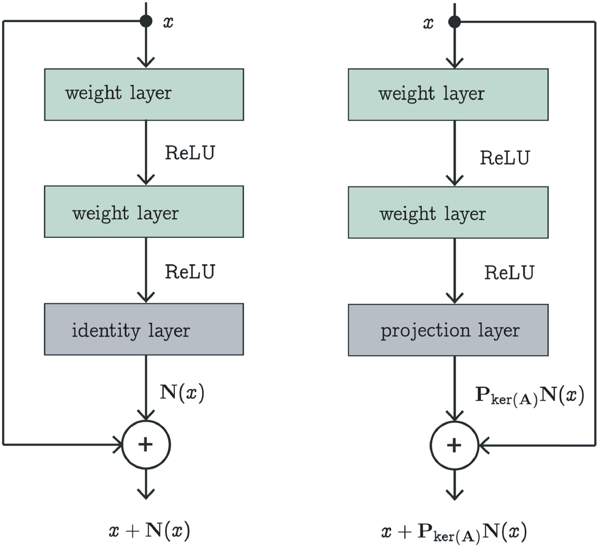
An example of a standard residual network $\newcommand{\N}{{\mathbb N}} \newcommand{\XX}{X} \newcommand{\Id}{{\rm Id}} \newcommand{\NN}{\mathbf{N}} \Id_{\XX} + \NN$ and a layered null space network $\newcommand{\N}{{\mathbb N}} \newcommand{\XX}{X} \newcommand{\Ao}{\mathbf A} \newcommand{\Id}{{\rm Id}} \newcommand{\NN}{\mathbf{N}} \Id_{\XX} + (\Id_{\XX} - \Ao^{+} \Ao) \NN$ both with depth $L=2$ (i.e. two weight layers) are shown in figure 2.

Zoom In Zoom Out Reset image size

Remark 3.3. Throughout the following we assume that $\newcommand{\N}{{\mathbb N}} \newcommand{\XX}{X} \newcommand{\Ao}{\mathbf A} \newcommand{\Id}{{\rm Id}} \newcommand{\NN}{\mathbf{N}} \newcommand{\nsn}{\mathbf{L}} \nsn = \Id_{\XX} + (\Id_{\XX} - \Ao^{+} \Ao) \NN$ is a given null-space network. Following the deep learning philosophy, the network would be selected from a parameterized family $\newcommand{\nsn}{\mathbf{L}} (\nsn_\theta)_{\theta \in \theta}$ based on given training data. A possible training strategy is presented in appendix. The results below hold for any null space network where the Lipschitz constant is finite. It is widely accepted that the Lipschitz constant in typically trained networks is reasonably small. As the error constant depends on the Lipschitz constants of the network it is desirable to keep the Lipschitz constant small. The proposed training strategy also accounts for this issue in the layered neural networks according to definition 3.1.

Another simple way of constructing a null space network is to add a data consistency layer to an existing network. To be specific, let $\newcommand{\nsn}{\mathbf{L}} \nsn_0$ be any trained network. Then one obtains a null space network by considering

$$\begin{align} \newcommand{\e}{{\rm e}} \newcommand{\nsn}{\mathbf{L}} \newcommand{\Id}{{\rm Id}} \newcommand{\Ao}{\mathbf A} \newcommand{\XX}{X} \newcommand{\la}{\lambda} \displaystyle \label{eq:nulspace1} \nsn = \Id_{\XX} + (\Id_{\XX} - \Ao^{+} \Ao) (\nsn_0 - \Id_{\XX}). \nonumber \end{align} \tag{ 3.2 }$$

Moreover, one can easily show that $\newcommand{\norm}[1]{{\left\Vert#1\right\Vert}} \newcommand{\Ao}{\mathbf A} \newcommand{\nsn}{\mathbf{L}} \norm{x - \nsn \Ao^{+} \Ao x } \leqslant \norm{x - \nsn_0 \Ao^{+} \Ao x}$ for every $x \in X$. Hence the null space network is always better in terms of reconstruction error than the original network for recovering $x$ from data $\newcommand{\Ao}{\mathbf A} y= \Ao x$.

Let $\newcommand{\N}{{\mathbb N}} \newcommand{\XX}{X} \newcommand{\Ao}{\mathbf A} \newcommand{\Id}{{\rm Id}} \newcommand{\NN}{\mathbf{N}} \Id_{\XX} + (\Id_{\XX} - \Ao^{+} \Ao) \NN$ be a null-space network, possibly trained as described in appendix by approximately minimizing (A.1). Any such network belongs to the class of functions $\newcommand{\XX}{X} \newcommand{\Id}{{\rm Id}} \newcommand{\nun}{\boldsymbol{\Phi}} \Id_{\XX} + \nun$ by taking $\newcommand{\N}{{\mathbb N}} \newcommand{\XX}{X} \newcommand{\Ao}{\mathbf A} \newcommand{\Id}{{\rm Id}} \newcommand{\NN}{\mathbf{N}} \newcommand{\nun}{\boldsymbol{\Phi}} \nun = (\Id_{\XX} - \Ao^{+} \Ao) \NN$. Consequently, the convergence theory of section 2 applies. In particular, theorem 2.4 shows that a regularization $\newcommand{\al}{\alpha} \newcommand{\Bo}{\mathbf B} (\Bo_\al)_{\al >0}$ of the Moore–Penrose generalized inverse defines a $\newcommand{\nun}{\boldsymbol{\Phi}} \nun$-regularization method via $\newcommand{\R}{{\mathbb R}} \newcommand{\N}{{\mathbb N}} \newcommand{\al}{\alpha} \newcommand{\XX}{X} \newcommand{\Ao}{\mathbf A} \newcommand{\Bo}{\mathbf B} \newcommand{\Ro}{\mathbf R} \newcommand{\Id}{{\rm Id}} \newcommand{\NN}{\mathbf{N}} \Ro_\al := (\Id_{\XX} + (\Id_{\XX} - \Ao^{+} \Ao) \NN) \Bo_\al$. Additionally, theorem 2.8 yields convergence rates for the regularization $\newcommand{\R}{{\mathbb R}} \newcommand{\al}{\alpha} \newcommand{\Ro}{\mathbf R} (\Ro _\al)_{\al >0}$ of $\newcommand{\Ao}{\mathbf A} \newcommand{\nun}{\boldsymbol{\Phi}} \Ao^{\nun}$.

In some cases, the projection $\newcommand{\XX}{X} \newcommand{\Po}{\mathbf P} \newcommand{\Ao}{\mathbf A} \newcommand{\Id}{{\rm Id}} \Po_{\ker(\Ao)} = \Id_{\XX} - \Ao^{+} \Ao$ might be costly to be computed exactly. For that purpose, in this section we derive more general regularization methods that include approximate evaluations of $\newcommand{\Ao}{\mathbf A} \Ao^{+} \Ao$.

Theorem 3.4. Let $\newcommand{\N}{{\mathbb N}} \newcommand{\XX}{X} \newcommand{\Ao}{\mathbf A} \newcommand{\Id}{{\rm Id}} \newcommand{\NN}{\mathbf{N}} \newcommand{\nsn}{\mathbf{L}} \nsn = \Id_{\XX} + (\Id_{\XX} - \Ao^{+} \Ao) \NN$ be a null space network and set $\newcommand{\ran}{{\rm ran}} \newcommand{\M}{{\mathcal M}} \newcommand{\nsn}{\mathbf{L}} \M := \ran(\nsn)$. Suppose $\newcommand{\al}{\alpha} \newcommand{\Bo}{\mathbf B} ((\Bo_\al)_{\al >0}, \al^\star)$ is a regularization method for $\newcommand{\signal}{x} \newcommand{\data}{y} \newcommand{\Ao}{\mathbf A} \Ao \signal = \data$. Moreover, let $\newcommand{\al}{\alpha} \newcommand{\Qo}{\mathbf Q} (\Qo_\al)_{\al >0}$ be a family of bounded operators on $\newcommand{\XX}{X} \XX$ with $\newcommand{\al}{\alpha} \newcommand{\snorm}[1]{\Vert#1\Vert} \newcommand{\Po}{\mathbf P} \newcommand{\Qo}{\mathbf Q} \newcommand{\Ao}{\mathbf A} \snorm{\Qo_\al - \Po_{\ker(\Ao)}} \to 0$ as $\newcommand{\al}{\alpha} \al \to 0$. Then, the pair $\newcommand{\R}{{\mathbb R}} \newcommand{\al}{\alpha} \newcommand{\Ro}{\mathbf R} ((\Ro_\al)_{\al >0}, \al^\star)$ with

$$\begin{align} \newcommand{\e}{{\rm e}} \newcommand{\NN}{\mathbf{N}} \newcommand{\Id}{{\rm Id}} \newcommand{\Ro}{\mathbf R} \newcommand{\Bo}{\mathbf B} \newcommand{\Qo}{\mathbf Q} \newcommand{\XX}{X} \newcommand{\al}{\alpha} \newcommand{\N}{{\mathbb N}} \newcommand{\R}{{\mathbb R}} \displaystyle \Ro_\al := (\Id_{\XX} + \Qo_\al \NN) \circ \Bo_\al \nonumber \end{align} \tag{ 3.3 }$$

is a $\newcommand{\nun}{\boldsymbol{\Phi}} \nun$-regularization method for $\newcommand{\signal}{x} \newcommand{\data}{y} \newcommand{\Ao}{\mathbf A} \Ao \signal = \data$. In particular, the family $\newcommand{\R}{{\mathbb R}} \newcommand{\al}{\alpha} \newcommand{\Ro}{\mathbf R} (\Ro_\al)_{\al >0}$ is a regularization of $\newcommand{\Ao}{\mathbf A} \newcommand{\nun}{\boldsymbol{\Phi}} \Ao^{\nun}$.

Proof. We have

$$\begin{align} \newcommand{\e}{{\rm e}} \newcommand{\nun}{\boldsymbol{\Phi}} \newcommand{\NN}{\mathbf{N}} \newcommand{\Id}{{\rm Id}} \newcommand{\Bo}{\mathbf B} \newcommand{\Ao}{\mathbf A} \newcommand{\Qo}{\mathbf Q} \newcommand{\Po}{\mathbf P} \newcommand{\XX}{X} \newcommand{\data}{y} \newcommand{\snorm}[1]{\Vert#1\Vert} \newcommand{\norm}[1]{{\left\Vert#1\right\Vert}} \newcommand{\la}{\lambda} \newcommand{\al}{\alpha} \newcommand{\N}{{\mathbb N}} \displaystyle \label{eq:Q} &\norm{(\Id_{\XX} + \Qo_\al \NN) \circ \Bo_\al (\data^\delta) - \Ao^{\nun}\data }\nonumber \\ &\leqslant \norm{(\Id_{\XX} + \Po_{\ker(\Ao)} \NN) \circ \Bo_\al (\data^\delta) - \Ao^{\nun}\data } + \snorm{\Qo_\al - \Po_{\ker(\Ao)}} \, \snorm{\NN \Bo_{\al} (\data^\delta)}. \nonumber \end{align} \tag{ 3.4 }$$

The claim follows from theorem 2.4. □

Theorem 3.5. Let $\newcommand{\N}{{\mathbb N}} \newcommand{\XX}{X} \newcommand{\Ao}{\mathbf A} \newcommand{\Id}{{\rm Id}} \newcommand{\NN}{\mathbf{N}} \newcommand{\nsn}{\mathbf{L}} \nsn = \Id_{\XX} + (\Id_{\XX} - \Ao^{+} \Ao) \NN$ be a null space network and set $\newcommand{\ran}{{\rm ran}} \newcommand{\M}{{\mathcal M}} \newcommand{\nsn}{\mathbf{L}} \M := \ran(\nsn)$. Let $\mu >0$, suppose $\newcommand{\al}{\alpha} \newcommand{\kl}[1]{\left(#1\right)} \kl{g_\alpha}_{\al >0}$ satisfies the assumptions of theorem 2.8, and let $\newcommand{\al}{\alpha} \newcommand{\Qo}{\mathbf Q} (\Qo_\al)_{\al >0}$ be a family of bounded operators on $\newcommand{\XX}{X} \XX$ with $\newcommand{\al}{\alpha} \newcommand{\snorm}[1]{\Vert#1\Vert} \newcommand{\Po}{\mathbf P} \newcommand{\Qo}{\mathbf Q} \newcommand{\Ao}{\mathbf A} \snorm{\Qo_\al - \Po_{\ker(\Ao)}} = \mathcal{O}(\alpha^\mu)$. Consider the regularization $\newcommand{\R}{{\mathbb R}} \newcommand{\al}{\alpha} \newcommand{\Ro}{\mathbf R} (\Ro_\al)_{\al>0}$ with

$$\begin{align} \newcommand{\e}{{\rm e}} \newcommand{\NN}{\mathbf{N}} \newcommand{\Id}{{\rm Id}} \newcommand{\Ro}{\mathbf R} \newcommand{\Ao}{\mathbf A} \newcommand{\Qo}{\mathbf Q} \newcommand{\XX}{X} \newcommand{\al}{\alpha} \newcommand{\N}{{\mathbb N}} \newcommand{\R}{{\mathbb R}} \displaystyle \Ro_\al := (\Id_{\XX} + \Qo_\al \NN) \circ g_\al(\Ao^*\Ao) \Ao^*. \nonumber \end{align} \tag{ 3.5 }$$

Then, the parameter choice $\newcommand{\al}{\alpha} \al^\star \asymp ({\delta}/{\rho})^{\frac{2}{2\mu+1}}$ yields the convergence rate results $\newcommand{\R}{{\mathbb R}} \newcommand{\al}{\alpha} \newcommand{\snorm}[1]{\Vert#1\Vert} \newcommand{\signal}{x} \newcommand{\Ro}{\mathbf R} \snorm{\Ro_{\al^\star(\delta, y^\delta)} (y^\delta) - \signal } = \mathcal{O}(\delta^{\frac{2\mu}{2\mu+1}})$ for any $\newcommand{\ran}{{\rm ran}} \newcommand{\signal}{x} \newcommand{\Ao}{\mathbf A} \newcommand{\nsn}{\mathbf{L}} \signal \in \ran(\nsn (\Ao^*\Ao)^\mu)$.

Proof. Follows from the estimate (3.4) with $\newcommand{\al}{\alpha} \newcommand{\Ao}{\mathbf A} \newcommand{\Bo}{\mathbf B} \Bo_\al = g_\al(\Ao^*\Ao) \Ao^*$ and theorem 2.8. □

One might use $\newcommand{\ph}{\varphi} \newcommand{\al}{\alpha} \newcommand{\Qo}{\mathbf Q} \newcommand{\Ao}{\mathbf A} \newcommand{\Bo}{\mathbf B} \Qo_\al = \Bo_{\phi(\al)} \Ao$ as a possible approximation to $\newcommand{\Po}{\mathbf P} \newcommand{\Ao}{\mathbf A} \Po_{\ker(\Ao)^\bot} = \Ao^{+} \Ao$ for some function $\newcommand{\ph}{\varphi} \phi \colon [0, \infty) \to [0, \infty)$. In such a situation, one can use existing software packages (for example, for the filtered backprojection algorithm and the discrete Radon transform in case of computed tomography) for evaluating $\newcommand{\ph}{\varphi} \newcommand{\al}{\alpha} \newcommand{\Bo}{\mathbf B} \Bo_{\phi(\al)}$ and $\newcommand{\Ao}{\mathbf A} \Ao$.