
Abstract
We study a Bayesian inverse problem arising in the context of resin transfer molding (RTM), which is a process commonly used for the manufacturing of fiber-reinforced composite materials. The forward model is described by a moving boundary problem in a porous medium. During the injection of resin in RTM, our aim is to update, on the fly, our probabilistic knowledge of the permeability of the material as soon as pressure measurements and observations of the resin moving domain become available. A probabilistic on-the-fly characterisation of the material permeability via the inversion of those measurements/observations is crucial for optimal real-time control aimed at minimising both process duration and the risk of defects formation within RTM. We consider both one-dimensional (1D) and two-dimensional (2D) forward models for RTM. Based on the analytical solution for the 1D case, we prove existence of the sequence of posteriors that arise from a sequential Bayesian formulation within the infinite-dimensional framework. For the numerical characterisation of the Bayesian posteriors in the 1D case, we investigate the application of a fully-Bayesian sequential Monte Carlo method (SMC) for high-dimensional inverse problems. By means of SMC we construct a benchmark against which we compare performance of a novel regularizing ensemble Kalman algorithm (REnKA) that we propose to approximate the posteriors in a computationally efficient manner under practical scenarios. We investigate the robustness of the proposed REnKA with respect to tuneable parameters and computational cost. We demonstrate advantages of REnKA compared with SMC with a small number of particles. We further investigate, in both the 1D and 2D settings, practical aspects of REnKA relevant to RTM, which include the effect of pressure sensors configuration and the observational noise level in the uncertainty in the log-permeability quantified via the sequence of Bayesian posteriors. The results of this work are also useful for other applications than RTM, which can be modelled by a random moving boundary problem.
Export citation and abstract BibTeX RIS

Original content from this work may be used under the terms of the Creative Commons Attribution 3.0 licence. Any further distribution of this work must maintain attribution to the author(s) and the title of the work, journal citation and DOI.
1. Introduction
In this paper we study the Bayesian inverse problem within the moving boundary setting motivated by applications in manufacturing of fiber-reinforced composite materials. Due to their light weight and high strength, as well as their flexibility to fit mechanical requirements and complex designs, such materials are playing a major role in automotive, marine and aerospace industries [3, 4, 27]. The moving boundary problem under consideration arises from resin transfer molding (RTM) process, one of the most commonly used processes for manufacturing composite materials. RTM consists of the injection of resin into a cavity mold with the shape of the intended composite part according to design and enclosing a reinforced-fiber preform previously fabricated. The next stage of RTM is curing of the resin-impregnated preform, which may start during or after the resin injection. Once curing has taken place, the solidified part is demolded from the cavity mold. In the present work we are concerned with the resin injection stage of RTM under the reasonable assumption that curing starts after resin has filled the preform. Though the current study is motivated by RTM, the results can be also used for other applications where a moving boundary problem is a suitable model.
We now describe the forward model (see further details in [3, 38, 47]). Let  ,
,  , be an open domain representing a physical domain of a porous medium with the permeability
  and porosity φ. The boundary of the domain
  is
is  , where
  is the inlet,
  is the perfectly sealed boundary, and
  is the outlet. The domain
  is initially filled with air at a pressure p0. This medium is infused with a fluid (resin) with viscosity μ through an inlet boundary
  at a pressure pI and moves through
  occupying a time-dependent domain
  , which is bounded by the moving boundary
  and the appropriate parts of
  . An example of the physical configuration of this problem in 2D is illustrated in figure 1.
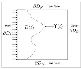
Figure 1. An example of the physical configuration of the moving boundary problem.
Download figure:
Standard image High-resolution imageThe forward problem for the pressure of resin  consists of the conservation of mass

where the flux  is given by Darcy's law

with the following initial and boundary conditions


Here  is the velocity of the point x on the moving boundary
  in the normal direction at x,
  and
and  are the unit outer normals to the corresponding boundaries.
We remark that for definiteness we have assumed that at the initial time the moving boundary  coincides with the inlet boundary
  and that the constant pressure condition is imposed at the inlet. It is not difficult to carry over the inverse problem methodology considered in this paper to other geometries and other conditions on the inlet (e.g. constant rate). Further, in two (three) dimensional RTM settings one usually models permeability via a second (third)-order permeability tensor to take into account anisotropic structure of the media [3, 38] but here for simplicity of the exposition the permeability
  is a scalar function. Again, the developed methodology is easy to generalize to the tensor case.
Let us note that in the 1D case the nonlinear problem (1)–(9) is analytically simple and admits a closed form solution (see section 2 and [38]) but the two and three dimensional cases are much more complicated and analytical solution is in general not available. We remark that in two and three dimensional cases the resin can race around low permeability regions and the front  can become discontinuous creating macroscopic voids behind the main front (see further details in [3, 38]) but in this paper we ignore such effects which deserve further study.
It has been extensively recognized [13, 14, 30, 31, 37, 42] that imperfections in a preform that arise during its fabrication and packing in the molding cavity can lead to variability in fiber placement which results in a heterogenous highly-uncertain preform permeability. In turn, these unknown heterogeneities in permeability of the preform give rise to inhomogeneous resin flow patterns which can have profound detrimental effect on the quality of the produced part, reducing its mechanical properties and ultimately leading to scrap. To limit these undesirable effects arising due to uncertainties, conservative designs are used which lead to heavier, thicker and, consequently, more expensive materials aimed at avoiding performance being compromised. Clearly, the uncertainty quantification of material properties is essential for making RTM more cost-effective. One of the key elements in tackling this problem is to be able to quantify, in real time, the uncertain permeability, which can, in turn, be used in active control systems aimed at reducing the risk of defects formation.
In this work we assume that  ,
,  ,
,  ,
,  , pI, p0, μ and φ are known deterministic parameters while the permeability
  is unknown. Our objective is within the Bayesian framework to infer
  or, more precisely, its natural logarithm
  from measurements of pressure
  at some sensor locations as well as measurements of the front
  , or alternatively, of the time-dependent domain
  at a given time t > 0. We put special emphasis on computational efficiency of the inference, which is crucial from the applicable point of view.
1.1. Practical approaches for permeability estimation in fiber-reinforced composites
While the estimation of preform permeability during resin injection in RTM is clearly an inverse problem constrained by a moving boundary PDE such as (1)–(9), most existing practical approaches pose the estimation of permeability in neither a deterministic nor stochastic inverse problems framework. For example, the very extensive review published in 2010 [41] reveals that most conventional methods for measuring permeability assume that (i) the material permeability tensor is homogenous and (ii) the flow is 1D (including 2D radial flow configurations). Under these assumptions the resin injection in RTM can be described analytically, via expressions derived from Darcy's law, which enable a direct computation of the permeability in terms of quantities that can be measured before or during resin injection. These conventional methods suffer from two substantial practical limitations. First, they do not account for the heterogenous structure of the preform permeability, and although they provide an estimate of an effective permeability, this does not enable the prediction of the potential formation of voids and dry spots. Second, those conventional methods compute the permeability in an off-line fashion (i.e. before RTM) with specific mold designs that satisfy the aforementioned assumptions intrinsic to those methods (e.g. rectangular flat molds). This second limitation is not only detrimental to the operational efficiency of RTM but also neglects the potential changes in permeability that can results from encapsulating the preform in cavities with complex designs.
Some practical methodologies for online (i.e. during resin injection) estimation of heterogenous permeability have been proposed in [36, 49]. While these approaches seem to address the aforementioned limitations of conventional methods, they also use a direct approach for the estimation of permeability which faces unresolved challenges. As an example, let us consider the recent work of [49] which uses an experimental configuration similar to the one described in figure 1 and which, by using pressure measurements from sensors located within the domain occupied by the preform, computes a finite-difference approximation of the normal flux to the front  . In addition, by means of images from CCT cameras, seepage velocity of the resin front is computed in [49]; this velocity is nothing but
  defined by (5) in the context of the moving boundary problem (1)–(9). Under the assumption that μ and φ are known, the approach proposed in [49] consists of finding

with  and
and  computed from measurements as described above. This approach offers a practical technique to estimating κ on the moving front and can then potentially infer the whole permeability field during the resin injection in RTM. However, from the mathematical inverse problems perspective, this ad-hoc approach is not recommended as it involves differentiating observations of pressure data for the computation of
  . Indeed, it is well-known [23] that differentiation of data is an ill-posed problem that requires regularization. In addition, rather than an inverse problem, the least-squares formulation in (10) is a data fitting exercise that excludes the underlying constraint given by the moving boundary problem and which entails a global effect induced by κ. As a result, the estimate of permeability obtained via (10) has no spatial correlation and thus fails to provide an accurate global estimate of the permeability field.
The recent work of [29] demonstrates considerable advantages of using systematic data assimilation approaches to infer permeability during the resin injection of RTM. By means of a standard ensemble Kalman methodology for data assimilation, the approach of [29] uses measurements from visual observations of the front location to produce updates of the preform permeability within the context of a discrete approximation of the moving boundary problem (1)–(9). While the methodology used in [29] is focused in producing deterministic estimates, the standard Kalman methodology can be potentially used to quantify uncertainty in preform permeability. However, it has been shown that standard Kalman methodologies, such as the one used in [29], could result in unstable estimates unless further regularisation to the algorithm is applied [18].
In addition to the lack of an inverse problem framework that can lead to unstable and ultimately inaccurate estimates of the permeability in resin injection of RTM, most existing approaches (i) do not incorporate the uncertainty in the observed variables and (ii) do not quantify uncertainty in the estimates of the permeability of preform. It is indeed clear from our literature review that the estimation of permeability of preform during resin injection deserves substantial attention from an inverse problems perspective capable of quantifying uncertainty inherent to the fabrication and packing of the preform.
1.2. The Bayesian approach to inverse problems
In this paper we propose the application of the Bayesian approach to inverse problems [46] in order to infer the logarithm of the permeability  , from observations
  collected at some prescribed measurement/observation times
  during the resin injection in RTM. At each time tn we observe a vector, yn, that contains noisy measurements of resin pressure from sensors as well as some information of the moving domain (or alternatively front location) observed, for example, via CCT cameras or dielectric sensors [32]. In the Bayesian approach, the unknown
  is a random function that belongs to a space of inputs X. A prior probability measure
  on u must be specified before the data are collected; this enables us to incorporate prior knowledge which may include design parameters as well as the uncertainty that arises from preform fabrication (i.e. prior to resin injection). In our work we consider Gaussian priors which have been identified as adequate for characterizing the aforementioned uncertainty in log-permeability from the preform fabrication [30, 31, 50] (see also references therein).
At each observation time tn during the infusion of resin in RTM, we then pose the inverse problem in terms of computing,  , the (posterior) probability measure of the log-permeability conditioned on measurements
  . Each posterior
  then provides a rigorous quantification of the uncertainty in the log-permeability field given all available measurements up to the time tn. Knowledge of each of these posteriors during RTM can then be used to compute statistical moments of the log-permeability under
  (e.g. mean, variance) as well as expectations of quantities of interest that may be needed for the real-time optimization of controls (e.g. pressure injection) in RTM.
Although the proposed application of the Bayesian formulation assumes Gaussian priors, the nonlinear structure of the PDE problem, that describes resin injection in RTM, gives rise to a sequence of non-Gaussian Bayesian posteriors  which cannot be characterized in a closed form. A sampling approach is then required to compute approximations of these posteriors. Among existing sampling methodologies, Sequential Monte Carlo (SMC) samplers [1, 8, 22, 34] are particularly relevant for the formulation of the above described inverse problem as they provide a recursive mechanism to approximate the sequence of Bayesian posteriors
  . Markov Chain Monte Carlo (MCMC) approaches [9] can also be used to compute
  , at each observation time tn. However, conventional MCMC formulations do not exploit the sequential nature of the problem by enabling a recursive estimation of
  which is crucial for the optimisation of the RTM process via making use of active control systems.
Starting with J samples from the prior  ,
,  (i.i.d.), the idea behind SMC is to transform a system of weighted particles
  that define
  to an updated set
  that approximates
  as the new data yn collected at time tn become available. The weights
  are normalised (i.e.
  ,
,  ) and the empirical measure
converges to  as
as  (
( denotes the Dirac measure concentrated at w). Moreover, if
  denotes a quantity of interest of the unknown log-permeability
  , the weighted particles
  can be easily used to compute the sample mean
which converges (see for example [34]) to the expectation (under  ) of the quantity of interest
  .
.
The recursive computation of the weighted particles in SMC is suitable for the proposed application in RTM as it allows us to update, potentially in real time, our knowledge of the uncertainty in the log-permeability. However, producing accurate approximations of the Bayesian posteriors  in the context of the inference of preform log-permeability in RTM represents a substantial computational challenge that arises from the fact that these posterior measures are defined on a (infinite-dimensional) functional space. Upon discretization, these posteriors could be potentially defined on a very high-dimensional space. Unfortunately, it has been shown [5, 9] that standard Bayesian sampling methodologies such as standard SMC do not scale well with the dimension of the (discretized) unknown; this leads to unstable and ultimately inaccurate algorithms.
The recent works [9, 22] developed scalable (dimension independent) sampling algorithms for the approximation of the Bayesian posterior that arises from high-dimensional inverse problems. While these algorithms have a solid theoretical background that ensures their stability and convergence properties, achieving a desirable level of accuracy often comes at extremely high computational cost. More specifically, Bayesian methodologies, that provide approximation of the form (11) and that converge asymptotically to the underlying posterior measure  , often involve solving the forward model thousands or even millions of times. In the context of the inverse problem for RTM, the numerical solution of the moving boundary (forward) problem in 2D or 3D settings is computationally very intensive. Therefore, the sequential approximation of the Bayesian posteriors of preform's log-permeability must be conducted with scalable computational efficiency so that it can be realistically used within a near real-time optimization loop for RTM. In the proposed work we develop a computational inverse framework that possess such computational efficiency with the ultimate aim of the real-time uncertainty quantification of the reinforced preform's log-permeability.
1.3. Contributions of this work
The contributions of this article are the following:
- (A)A Bayesian formulation of the inverse problem to infer log-permeability from sequential data collected during resin injection in RTM. Both the 2D forward model described by (1)–(9) as well as the corresponding 1D version are considered. For the 1D case, we show that application of the infinite-dimensional Bayesian framework of [46] leads to well-posedness of the sequence of Bayesian posteriors.
- (B)Application of a state-of-the-art SMC framework [22] for the approximation of the sequence of Bayesian posteriors
 that arises from the Bayesian formulation. Our use of SMC serves two purposes. First, the SMC framework motivates construction of a novel regularizing ensemble Kalman algorithm (REnKA) that aims at approximating this sequence of posteriors in a computationally efficient manner, thus suitable for its implementation in a practical setting of RTM. Second, we use a Benchmark obtained by SMC application in order to test accuracy of REnKA.
 - (C)Numerical investigation of the accuracy and robustness of the proposed REnKA scheme in the 1D case; this involves constructing, via the SMC sampler of [22], accurate approximations of the posteriors that we use as Benchmark against which we compare the proposed REnKA. The advantages of REnKA in terms of accuracy versus computational cost are showcased by comparing it with the implementation of a low-resolution SMC whose computational cost is comparable to REnKA's.
- (D)Application of REnKA for further investigations of the Bayesian inverse problem in both 1D and 2D. In particular for the 1D case we conduct a numerical investigation of the added value of assimilating the front location relative to the number of pressure sensors. Since the number of pressure sensors that can be physically deployed for preform permeability monitoring in RTM is usually limited, this investigation aims at providing practitioners with guidelines for the number of sensors that can accurately infer preform permeability alongside with its uncertainty. In addition, for the 1D case we study the effect of the frequency of the observations, as well as the observational noise level on the inference of the log-permeability. We further apply REnKA to the 2D forward model and, analogous to the 1D case, we study the effect that the number of pressure sensors have on the inferred log-permeability.

The rest of the paper is organized as follows. In section 2 we introduce the Bayesian inverse problem of inferring the permeability of a porous media in a 1D moving boundary problem for resin injection in RTM. In section 3 we discuss and apply SMC to approximate the Bayesian posteriors that arise from the Bayesian approach. In section 4 we introduce REnKA and then conduct, via numerical experiments with the 1D RTM model, a numerical investigation of its approximation properties relative to its computational cost. In section S1 of the supplementary material (stacks.iop.org/IP/34/105002/mmedia) SupMat we further investigate relevant practical aspects of the inverse problem in 1D including the study of the effect of the number of pressure sensors as well as the noise level on accuracy of the inferred log-permeability and its uncertainty. In section 5 we demonstrate the applicability of REnKA to approximate the Bayesian inverse problem in the 2D RTM model described earlier. Some conclusions are presented in section 6.
2. Bayesian inversion of a 1D RTM model
In this section we apply the Bayesian approach to infer log-permeability in the context of the 1D version of the forward problem defined in (1)–(9). The corresponding 1D moving boundary problem induces a sequence of forward maps that we define in section 2.1 and that we aim at inverting with the Bayesian formalism that we introduce in section 2.2. This sequence of 1D forward maps admits a closed-form solution that can be numerically approximated at a very low computational cost. This will enable us in section 3 to obtain accurate numerical approximations of the solution to the Bayesian inverse problem; we use these accurate approximations as a benchmark for assessing the approximation properties of the ensemble Kalman algorithm that we introduce in section 4.
2.1. The forward 1D RTM model
Let us consider a 1D porous media with physical domain ![$ \newcommand{\e}{{\rm e}} D^{\ast}\equiv [0, x^{\ast}]\subset \mathbb{R}$](https://content.cld.iop.org/journals/0266-5611/34/10/105002/revision2/ipaad1ccieqn073.gif) . As before, we denote by
. As before, we denote by  (
( ) and
) and  the permeability and porosity of the porous medium, respectively. Resin with viscosity μ is injected at x = 0 at a pressure pI. The pressure at the moving front (outlet)
  is prescribed and equal to p0. The initial pressure distribution before injection is also set to p0. For convenience of the subsequent analysis, we parameterize the permeability in terms of its natural logarithm
  . The pressure
  and the moving front
  are given by the solution to the following model


The solution to (13)–(17) can be obtained analytically by the following proposition (see [3, 38, 47]).
Proposition 2.1. Given ![$ \newcommand{\e}{{\rm e}} u\in X\equiv C[0, x^{\ast}]$](https://content.cld.iop.org/journals/0266-5611/34/10/105002/revision2/ipaad1ccieqn081.gif) , let us define
, let us define

The unique solution  ,
,  of (13)–(17) is given for
  by
by


The quantity of interest arising from the RTM injection model is the so-called filling time: the time it takes the front  to reach the right boundary of the domain of interest
 ![$[0, x^{\ast}]$](https://content.cld.iop.org/journals/0266-5611/34/10/105002/revision2/ipaad1ccieqn086.gif) . Filling time, denoted by
. Filling time, denoted by  , is defined by
  . From (19) and the definition in (18) it follows [38] that
  is given by

Note that the parameters p0 and pI are prescribed control variables and thus known. In addition, we assume that μ and φ are known constants. As stated earlier, we are interested in the inverse problem of estimating the permeability, or more precisely its natural logarithm  given time-discrete measurements of the front location as well as the pressure from M sensors located at
 ![$\{x_{m}\}_{m=1}^{M}\subset [0, x^{\ast}]$](https://content.cld.iop.org/journals/0266-5611/34/10/105002/revision2/ipaad1ccieqn091.gif) . We denote by
. We denote by  the set of N observation times. For fixed (assumed known) parameters pI, p0, φ and μ, the solution to the PDE model (13)–(17) induces the nth forward map
 ![$ \newcommand{\cG}{{\mathcal G}} \cG_{n}:C[0, x^{\ast}]\to \mathbb{R}^{M+1}$](https://content.cld.iop.org/journals/0266-5611/34/10/105002/revision2/ipaad1ccieqn093.gif) defined by
defined by

Given  , the evaluation of the forward map
  predicts the location of the front and the pressure at the sensor locations at the time t = tn. Since observation times are prescribed before the experiment, there is no assurance that for a given u, the corresponding filling time satisfies
  for all
  . In other words, the front could reach the right end of the domain before we observe it at time tn. In a real experimental setting, the process stops at time
  . However, in the inverse problem of interest here, observation times are selected beforehand, and the search of optimal u's within the Bayesian calibration of the nth forward map can lead to filling times greater than some observation times. In this case
  , the definition (22) yields
 ![$ \newcommand{\cG}{{\mathcal G}} \newcommand{\Ga}{\Upsilon} \cG_{n}(u) =[\Ga(\tau^{\ast}), \{\,p(x_{m}, \tau^{\ast})\}_{m=1}^{M}]^{T}$](https://content.cld.iop.org/journals/0266-5611/34/10/105002/revision2/ipaad1ccieqn100.gif) .
.
The following theorem ensures the continuity of the forward map, which is necessary for justifying the application of the Bayesian framework in section 2.2.2.
Theorem 2.2. The forward map ![$ \newcommand{\cG}{{\mathcal G}} \cG_{n}:C[0, x^{*}]\to \mathbb{R}^{M+1}$](https://content.cld.iop.org/journals/0266-5611/34/10/105002/revision2/ipaad1ccieqn101.gif) is continuous.
is continuous.
For the proof of this theorem, see appendix A.
In the following subsection we apply the Bayesian framework for inverse problems in order to invert observations of  .
.
Remark 2.3. We note that for the present work the porosity φ is an assumed known constant; our objective is to infer the log-permeability  . However, the Bayesian methodology that we apply can be extended to the case where the unknown is not only
  but also φ, and can include the case where
  is a spatial function defined on the physical domain
  .
.
2.2. The Bayesian inverse problem
Suppose that, at each observation time t = tn, we collect noisy measurements of the front location as well as pressure measurements from sensors. We denoted these measurement by  and
and  , respectively. Our aim is to solve the inverse problem of estimating the log permeability
  given all the data
  up to time t = tn. We assume that the aforementioned observations are related to the unknown
  , via the forward map (22), in terms of


where  and
and  are realizations of Gaussian noise with zero mean and covariance
  and
and  , respectively, i.e.
  and
and  (i.i.d.). For simplicity we assume that both measurements of the front location and pressures are uncorrelated in time. We additionally assume that
  and
and  are uncorrelated for all
  .
.
Note that (23) and (24) can be written as

with

Remark 2.4. Due to the nature of the RTM problem, we have that the pressure p(xm,t) at each sensor xm should increase with time as well as the fact that  . However, the Gaussian noise in (23) and (24) can make the observations
  and
and  'unphysical'. In practice, observations need to be post-processed before using them for the Bayesian inverse problem and unphysical
  should be excluded. We leave the question of how to incorporate such a post-processing framework for future study. Here we follow the traditional point of view on data modeled via (23) and (24) and choose sufficiently small
  and
and  so that the probability of
  being unphysical is very low.
We adopt the Bayesian framework for inverse problems where the unknown  is a random field and our objective is to characterize the sequence of distributions of u conditioned on the observations which we express as
  . In other words, at each observation time t = tn we aim at computing the Bayesian posterior
  . From this distribution we can obtain point estimates of the unknown that can be used in real time to, for example, modify controls (e.g. pI). More importantly, as we stated in the Introduction, the aforementioned distribution enables us to quantify uncertainty not only of the unknown but also of quantities of interest that may be relevant to an optimization of resin injection in RTM.
Even though for the illustrative purposes the model presented in this section is discretized on a relatively low dimensional space (e.g. 60 cells), our aim is to introduce a general computational framework independent of the size of the discretized domain. We therefore consider an infinite-dimensional formulation of the Bayesian inverse problem for which the unknown u belongs to a functional space X. The discretization of the Bayesian inverse problem will be conducted at the last stage of the computational algorithm, when the posteriors are sampled/approximated. Thus, we are aiming at robust mesh-invariant computational algorithms.
2.2.1. The prior.
For the Bayesian approach that we adopt in this work, we require to specify a prior distribution  of the unknown, before the data are collected. This distribution comprises all our prior knowledge of the unknown and may include, for example, the regularity of the space of admissible solutions to the inverse problem. For the present work we consider Gaussian priors which have been used to characterize the uncertainty in the (log) permeability that arises from the preform fabrication [30, 31, 50] (see also references therein). In particular, here we consider stationary Gaussian priors
  with covariance operator
  that arises from the Wittle–Matern correlation function defined by [25, 28, 39, 43]:
where Γ is the gamma function, l is the characteristic length scale,  is an amplitude scale and
  is the modified Bessel function of the second kind of order ν. The parameter ν controls the regularity of the samples. It can be shown [11, 43] that, for any
  , if
, if  , then
 ![$u\in C[0, x^{\ast}]$](https://content.cld.iop.org/journals/0266-5611/34/10/105002/revision2/ipaad1ccieqn138.gif) almost-surely, i.e.
almost-surely, i.e. ![$\mu_{0}([0, x^{\ast}])=1$](https://content.cld.iop.org/journals/0266-5611/34/10/105002/revision2/ipaad1ccieqn139.gif) . This requirement, together with the continuity of the forward map ensures the well-posedness of the Bayesian inverse problems as we discuss in the next subsection. In the context of composite preform's permeability, it is natural to choose the mean
. This requirement, together with the continuity of the forward map ensures the well-posedness of the Bayesian inverse problems as we discuss in the next subsection. In the context of composite preform's permeability, it is natural to choose the mean  according to the log-permeability intended by the design of the composite part [38].
For computational purposes we use the prior to parametrize the unknown u in terms of its Karhunen–Loeve (KL) expansion [2]:

with coefficients uk and where  and
and  are the eigenvectors and eigenfunctions of
  , respectively. A random draw from the prior
  can then be obtained from (28) with drawing
  i.i.d.
2.2.2. The posterior.
From (25) and our Gaussian assumptions on the observational noise, it follows that for a fixed  , we have
  . Therefore, the likelihood of
  is given by

At a given time t = tn, the Bayesian posterior  is defined by the following infinite-dimensional version of Bayes's rule.
theorem Let  be the sequence of forward maps defined by (22) and let
  be the corresponding likelihood functions (29). Let
  be the prior distribution with correlation function (27). Then, for each
  , the conditional distribution of
  , denoted by
  , exists. Moreover,
  with the Radon–Nikodym derivative

where

Proof. The proof follows from the application of theorem 6.31 in [46] and the continuity of the forward maps (theorem 2.2) on a full  -measure set X. □
Note that from our assumption of independence of  , the right hand side of (30) is the likelihood of
  .
.
Remark 2.6. Due to the assumption of independence between front location and pressure measurements, the likelihood (29) can be expressed as

where

This enables us to define two particular cases of the inverse problem. The first case corresponds to the assimilation of only pressure measurements  , while in the second case only front location measurements
  are assimilated. Similar arguments to those that led to theorem 2.5 can be applied (with
  instead of
  ) to define the Bayesian posteriors
  and
and  associated to these two Bayesian inverse problems. In section S1 of the supplementary material SupMat we study these two particular cases with an eye towards understanding the added value of assimilating observations of the front location with respect to assimilating only pressure measurements.
3. Approximating the posteriors via sequential Monte Carlo method
In the previous section we have established the well-posedness of the Bayesian inverse problem associated to inferring the log-permeability in the 1D moving boundary problem (13)–(17). The solution of this inverse problem is the sequence of posterior measures  defined by theorem 2.5. As we discussed in section 1, these posteriors cannot be expressed analytically and so a sampling approach is then required to compute the corresponding approximations. As stated earlier, the sampling of each posterior
  (
( ) can be performed independently by, for example, Markov chain Monte Carlo (MCMC) methods. However, we reiterate that, for the present application SMC samplers are rather convenient as they exploit the sequential nature of the considered inverse problem by enabling a recursive approximation of the posterior measures as new data (in time) become available. Such recursive approximations of the posterior could enable practitioners to update their probabilistic knowledge of preform's log-permeability which is, in turn, essential to develop real-time optimal control strategies for RTM under the presence of uncertainty.
Recognizing that the inverse problem under consideration involves inferring a function potentially discretized on a very fine grid, it is vital to consider the application of SMC samplers such as the one introduced in [22], carefully designed for approximating measures defined on a high-dimensional space. In this section we review and apply this scheme for the approximation of the Bayesian posteriors  that we defined in the previous section. The aims of this section are to (i) provide a deeper quantitative understanding of the accuracy of the fully-Bayesian methodology of [22] with respect to its computational cost under practical computational conditions; (ii) provide a motivation for the proposed REnKA that we propose from this SMC sampler in section 4; and (iii) define accurate approximations of
  which we use as a benchmark for testing our REnKA scheme.
In section 3.1 we briefly discuss the essence of the standard SMC that we then use in sections 3.2–3.3 to review methodological aspects of the adaptive-tempering SMC sampler for high-dimensional inverse problems of [22]. We then apply this SMC in section 3.4 for the solution of the Bayesian inverse problem in the 1D case defined in the previous section. In section 3.5 we assess practical limitations of the SMC.
3.1. Standard SMC for Bayesian inference
As we discussed in the Introduction, starting with the prior  , the objective of SMC is to recursively compute an approximation of the sequence of Bayesian posteriors
  in terms of weighted particles. More specifically, assume that at the observation time tn, we have a set of J particles
  with, for simplicity, equal weights (
 ,
,  ), which provides the following particle approximation of
  :
:
The objective now is to construct a particle approximation of  , which includes the new data yn collected at time tn. In a standard SMC framework [8, 10, 33], this particle approximation is constructed by means of an importance sampling step with proposal distribution
  . To illustrate this methodology, let us first note formally that
where we have used

which can be obtained directly from theorem 2.5. An approximation of (35) can be obtained by
where
From (37) we see that the importance (normalized) weights  assigned to each particle
  define the following empirical (particle) approximation of
  :
:
However, the accuracy of such empirical approximation relies on  being sufficiently close to
  ; when this is not the case, after a few iterations (observation times) the algorithm may produce only a few particles with nonzero weights. This is a well-known issue of weight degeneracy that often arises from the application of empirical (importance sampling) approximations within the context SMC samplers [5]. Weight degeneracy is routinely measured in terms of the effective sample size (ESS) statistic [24]:
which takes a value between 1 and J;  when all weights are equal and
  when the distribution is concentrated at one single particle. A common approach to alleviate weight degeneracy is, for example, to specify a threshold for the ESS below which resampling (often multinomially) according to the weights
  is performed. Resampling discards particles with low weights by replacing them with several copies of particles with higher weights. The approximation of a sequence of measures via the combination of the importance sampling step followed with resampling leads to the sequential importance resampling (SIR) scheme [10].
It is important to note that the aforementioned resampling step in SIR can clearly lead to the lack of diversity in the population of resampled particles. This is, in turn, detrimental to the approximation of the sequence of posteriors. The general aim of the standard SMC approach is to diversify these particles by a mutation step with involves replacing them with samples from a Markov kernel  with invariant distribution
  . In the following subsection we provide a discussion of the aforementioned mutation in the context of the SMC sampler for high-dimensional inverse problem [22]. We refer the reader to [8, 10, 33, 34] for a thorough treatment of more standard SMC samplers.
3.2. SMC for high-dimensional inverse problems
The weight degeneracy in the importance sampling step described above is more pronounced when the two consecutive measures  and
and  differ substantially from each other. This has been particularly associated with complex (e.g. multimodal) measures defined in high-dimensional spaces. When the change from
  to
to  is abrupt, the importance sampling step can result in a sharp failure, whereby the approximation of
  is concentrated on a single particle [5]. Recent work for high-dimensional inference problems has suggested [1, 22] that further stabilization of the importance weights is needed by defining a smooth transition between
  and
and  . For the present work, we consider the annealing approach of [34, 35], where qn intermediate artificial measures
  are defined such that
  and
and  . These measures can be bridged by introducing a set of qn tempering parameters denoted by
  that satisfy
  and defining each
  as the probability measure with density proportional to
  with respect to
  . More specifically,
  satisfies

which, formally, implies

Note that when qn = 1,  and so expression (42) reduces to (36). We now follow the SMC algorithm for high-dimensional inverse problems as described in [22].
3.2.1. Selection step.
The first stage of the SMC approach of [22] is a selection step which consists of careful selection of the tempering parameters which define the intermediate measures  ; these are in turn approximated by the application of the SIR scheme described above. Let us then assume that at an observation time tn and iteration level r − 1, the tempering parameter
  has been specified, and that a set of particles
  provides the following approximation (with equal weights) of the intermediate measure
  :
:
From (42) we can see that the new tempering parameter  must be selected to ensure that
  is sufficiently small, so that the subsequent measure
  is close to
  thus preventing a sharp failure of the empirical approximation of
  (39). In particular, once the next tempering parameter
  is specified, we note from expression (42) that the importance weights for the approximation of
  are given by
Recognizing that the ESS in (40) quantifies weight degeneracy in SIR, the approach of [22] (see also [21]) proposes to define on-the-fly the next tempering parameter  by imposing a fixed, user-defined value Jthres on the ESS. More specifically,
  is defined by the solution to the following equation:
which may, in turn, be solved by a simple bisection algorithm on the interval ![$(\phi_{n, r-1}, 1]$](https://content.cld.iop.org/journals/0266-5611/34/10/105002/revision2/ipaad1ccieqn219.gif) . An approximation of
. An approximation of  is then given by the weighted particle set
  . If at the r − 1 level, we find that
  , it implies that no further tempering is required and thus one can simply define
  . We note that the number of tempering steps qn is random.
While the tempering approach described above is aimed at preventing ESS from falling below a specified threshold Jthres and thus avoiding a sharp failure of the empirical approximation of  , resampling is still required to discard particles with very low weights. Let us then denote by
  (
( ) the particles, with equal weights, that result from resampling with replacement of the set of particles
  according to the weights
  .
.
3.2.2. Mutation phase.
As stated in the preceding subsection, at the core of the SMC methodology is a mutation phase that adds diversity to the population of the resampled particles  . In the context of the tempering approach described above, this mutation is conducted by means of sampling from a Markov kernel
  with invariant distribution
  . Similar to the approach of [22], here we consider mutations given by running
  steps of an MCMC algorithm with
  as its target distribution. More specifically, we consider the preconditioned Crank–Nicolson (pcn)-MCMC method from [9] with target distribution
  and reference measure
  . Formally, these two measures are related by

The pcn-MCMC method for sapling  is summarised in algorithm 2 (see appendix B). Under reasonable assumptions this algorithm produces a
  -invariant Markov kernel [22]. The resulting particles denoted by
  (
( ) then provide the following particle approximation of
  :
:
where the convergence is proven in a suitable metric for measures [1]. Note that at the end of the iteration r = qn, the corresponding particle approximation  provides the desired approximation of the posterior that arises from the Bayesian inverse problem of interest. This SMC sampler is summarized in algorithm 3 (see appendix B).
Remark 3.1. For simplicity, here we use the resampling step at every iteration of the SMC sampler. However, whenever  (and so
  ) the resampling step can be skipped; this involves using the corresponding weighted particle approximation and modifying the formula for the incremental weights as discussed in [22, section 4.3].
3.3. A note on tempering
Let us define the following inverse of the increment in tempering parameters:

and note that  implies
  . In addition, expression (42) can be written as
where we have used the definition of the likelihood in (29). Informally, we can then interpret each iteration of the SMC sampler (at a given observation time tn) as the solution of a Bayesian inverse problem that consists of finding  given the prior
  and the data:

From (48) and the fact that  , it follows that
  . Therefore, (50) is nothing but the original problem (25) albeit with a noise
  that has an inflated covariance
  .
.
We also note that  plays the role of a regularization parameter in the sense that it controls the transition between
  and
and  . The larger the
  the smoother this transition. Alternatively, we can see that
  can be interpreted as a 'temperature' in the tempering scheme which, in turn, flattens out the likelihood function at the observation time tn. Clearly, more tempering will be required whenever
  is large; this can for example happen if the observational data are accurate (i.e. small
  ) and/or many observations are available.
The amount of tempering is controlled by the number of parameters obtained via (45). The greater the number of tempering parameters, the larger the  's which in turn indicates that more regularization is needed to ensure a stable transition between those measures. This has also, in turn, an associated increase in iterations and thus in computational cost.
3.3.1. Computational aspects of SMC.
The main computational cost of the SMC sampler previously discussed is attributed to the mutation step for which  steps of the pcn-MCMC algorithm are performed. At each observation time tn and iteration r, the SMC sampler then requires
  evaluations of the nth forward map
  . Therefore, the computational cost of computing
  is
is  , where gn denotes the computational cost of evaluating
  which, in turn, corresponds to solving the moving boundary problem from time t = 0 up to time tn. The total computational cost of computing the full sequence of posteriors
  is then

which is expressed in terms of gN, the cost of evaluating  (i.e. solving the forward model from time zero up to the final observation time).
The work of [22] has suggested that accurate approximations of the posterior via SMC samplers require, for example, values of  and J = 104. If we assume for a moment that only one observation time N = 1 is considered and that only one tempering step q1 = 1 is required to compute
  , the computational cost in this case would be approximately 105 times the cost of solving the forward model from time t = 0 up to time t1. Such cost would be clearly computationally prohibitive for practical applications, where the aforementioned forward simulation may take several minutes of CPU time. In particular, for the 2D or 3D version of the RTM process, the high computational cost of the SMC sampler becomes impractical. While reducing the values of J and
  may result in a more affordable computational cost, this is substantially detrimental to the level of accuracy of the SMC sampler as we show via numerical experiments in section 3.5. Alternatively, a parallel implementation of the J forward model evaluations can substantially reduce the cost of this algorithm, which in turn, scales by a factor of J. However, within the manufacturing industry, the availability of computer resources that can deliver
  parallel simulations is the exception rather than the norm.
3.4. Numerical examples with SMC
In this subsection we report the results from the numerical application of the SMC sampler discussed in the previous subsection. The objective is to approximate the sequence of Bayesian posteriors that arise from the 1D moving boundary problem defined in section 2 for the experimental set-up described in section 3.4.1. In section 3.4.2 we discuss the numerical results obtained via the SMC sampler with a very high number of particles which results in accurate approximations of the Bayesian posteriors. These approximations are then used in section 3.5 to assess the practical limitations of the scheme under certain choices of tunable parameters and number of particles. These limitations motivate the approximate methods that we propose in section 4.
3.4.1. Experimental set-up.
We consider a dimensionless version of the 1D model (13)–(17) which together with its numerical approximation is described in appendix C. The dimensionless values for the control variables are p0 = 1 and pI = 2. We use a Gaussian prior distribution  with the covariance operator
  that arises from the covariance function defined in (27). We numerically solve (off-line) the eigenvalue problem associated to the matrix that results from discretizing
  ; the corresponding eigenvector/eigenvalues are then stored for subsequent use in the parameterization of the log-permeability in the SMC sampler. The KL expansion (28) becomes a truncated sum with a number of elements equal to the the total number of eigenvalues of this matrix; these are, in turn, equal to the number of cells used for the discretization of the domain
 ![$D^{\ast}=[0, 1]$](https://content.cld.iop.org/journals/0266-5611/34/10/105002/revision2/ipaad1ccieqn275.gif) . No further truncation to this KL expansion is carried out. A few samples from the prior are displayed in figure 2 (right). Pointwise percentiles (0.02, 0.25, 0.5, 0.75 and 0.98) of the prior are displayed in figure 3 (top-left). Tuneable parameters of the prior for the present experiments are
. No further truncation to this KL expansion is carried out. A few samples from the prior are displayed in figure 2 (right). Pointwise percentiles (0.02, 0.25, 0.5, 0.75 and 0.98) of the prior are displayed in figure 3 (top-left). Tuneable parameters of the prior for the present experiments are  ,
,  , l = 0.05 and
  for all
  .
.

Figure 2. Left: true pressure field  and space-time measurement configuration with M = 9 sensors and N = 5 observation times. Middle: true pressure at observation times
  (curves) together with the corresponding synthetic data
  (dots). Right: samples from the prior.
Download figure:
Standard image High-resolution image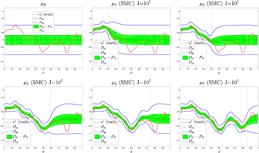
Figure 3. Top-left: percentiles of the prior log-permeability  . Top-Middle to bottom-right: percentiles of the posteriors
  obtained via SMC with large number of samples J = 105. Solid red line corresponds to the graph of the true log-permeability
  . Vertical dotted line indicates the location of the true front
  .
.
Download figure:
Standard image High-resolution imageIn order to generate synthetic data, we define the 'true/reference' log permeability field  whose graph (red curve) is displayed in figure 3 (top-left); this function is a random draw from the prior described above. We use
  in the numerical implementation of (13)–(17) in order to compute the true pressure field
  as well as the true front location
  . The plot of
  is shown in figure 2 (left) together with the space-time configuration of M = 9 pressure sensors and N = 5 observation times. The graphs of
  are shown in figure 2 (middle). The true locations of the front
  are 0.21, 0.40, 0.58, 0.73 and 0.87. Synthetic data are then generated by means of
  and
and  , where
  and
and  are Gaussian noise (see section 2.2) with standard deviations equal to 1.5% of the size of the noise-free observations. Synthetic pressure data
  are superimposed on the graphs of
  in figure 2 (middle). Synthetic front locations
  are 0.21, 0.39, 0.59, 0.74, 0.86. In order to avoid inverse crimes, synthetic data are generated by using a finer discretization (with 120 cells) than the one used to approximate the posteriors (with 60 cells).
3.4.2. Application of SMC.
In this subsection we report the application of the SMC sampler of [22] (see algorithm 3 in appendix B) which, as described in the preceding section, provides a particle approximation of each posterior that converges to the exact posterior measure  as the number of particles J goes to infinity. In order to achieve a high-level of accuracy we use J = 105 number of particles which is substantially larger compared to the number of particles (e.g. 103 to 104) often used in existing applications of SMC for high-dimensional inverse problems [8, 22]. In addition, we consider the selection of tunable parameters
  and
and  similar to the ones suggested in [22]. For each observation time tn, we store the ensemble of particles
  that approximates the corresponding posterior
  . From this ensemble, we compute the 0.02, 0.25, 0.5, 0.75, 0.98 posterior percentiles displayed in figure 3 (top-middle to bottom-right), where we also include the graph of the true log-permeability (red curve). The vertical line in these figures indicate the true location of the front
  at each observation time tn. We can clearly appreciate that the uncertainty band defined by these percentiles is substantially reduced as more observations (in time) are assimilated. In fact, the main reduction of the uncertainty is observed in the region of the moving domain
 ![$ \newcommand{\Ga}{\Upsilon} \newcommand{\re}{{\rm Re}} \renewcommand{\dag}{\dagger}D^{\dagger}(t_{n})=[0, \Ga^{\dagger}(t_{n})]$](https://content.cld.iop.org/journals/0266-5611/34/10/105002/revision2/ipaad1ccieqn307.gif) at the corresponding observation time tn. It is then clear that at each observation time tn, measurements collected from pressure sensors with
at the corresponding observation time tn. It is then clear that at each observation time tn, measurements collected from pressure sensors with  are not very informative of the log-permeability field. This comes as no surprise when we recognize that the pressure field given by (20) depends on the permeability field only in the region of the moving domain
  . In other words, the values of the permeability in the region defined by
  have no effect on p(x, tn); hence the nth likelihood function is independent of u in this region. We can indeed observe from figure 3 that the percentiles of the log-permeability in this region (see domain to the right of the vertical lines) is similar to those from the prior. However, due to the regularity of the log-permeability enforced in the prior
  , there is a smooth transition in the uncertainty band at the interface defined by the front location
  .
.
The number of intermediate tempering distributions that SMC adaptively computed to approximate the sequence of posteriors  were the following:

We use these numbers in (51) to compute the total computational cost of approximating the sequence  . The values of gn (i.e. cost of evaluating each
  ) are estimated by the average CPU time from 1000 simulations computed with different log-permeabilities sampled from the prior. We obtain that total cost is approximately
  times the cost of evaluation the 5th forward map
  (i.e. at the final observation time). Clearly, this computational cost is prohibitive for the two and three dimensional problems where, as stated earlier, evaluating the forward map can take several minutes of CPU time. For the present 1D case we are able to afford this cost due to the relatively low cost associated with solving the 1D moving boundary problem.
3.5. Reducing the cost of SMC by adjusting tunable parameters
Given the high computational cost of computing accurate approximations of the posteriors with SMC, it is reasonable to ask whether its computational cost can be reduced by adjusting the tunable parameters in (51). By reducing either the number of particles J and/or the number of MCMC steps  , we can achieve a substantial decrease in the computational cost. The selection of Jthresh also determines the computational cost as it, in turns, defines the number of tempering steps for each posterior. However, it is essential to understand the effect of decreasing these tunable parameters on accuracy of the SMC sampler. In this subsection we aim at understanding this effect by comparing the application of the SMC sampler with smaller number of particles J and different choices of the tunable parameters
  and Jthresh. This requires creating a Benchmark against which we can compare performance of SMC. The Benchmark is obtained by the highly-resolved characterization of the posteriors that we computed in the preceding section by using the SMC sampler with large number of particles (J = 105). In section S1 of the supplementary material SupMat we provide further discussions of the performance and diagnostics of the SMC sampler applied to approximate these posterior measures. These diagnostics offer evidence that the SMC sampler has been successfully applied, thereby providing accurate characterization of the posterior that we may use as a Benchmark to compare against the posteriors computed via algorithms with lower resolution/accuracy. The numerical investigation below is aimed at assessing SMC with different selections of ensemble size J as well as the tunable parameters
  and Jthresh.
For the reasons stated above, through the rest of the this and the following sections, we refer to the aforementioned highly-resolved SMC particle approximations (with J = 105) as the 'exact' sequence of posteriors  that we use for subsequent comparisons purposes. Moreover, for these comparisons we assume that the sample mean and variance of these SMC samples are exact approximations of the mean
  and variance
  of the posterior
  . In other words, we assume

where
Let us now consider the application of the SMC sampler for the following choices of small number of particles:  . We also consider three choices of the tunable parameter Jthresh (
 ) and two choices of
  (
( ). In figure 4 we show percentiles of the log-permeability posteriors
  (for
(for  and 5) obtained using the aforementioned SMC sampler for some of those choices of the number particles J, and with the same selection of tunable parameters
  ,
,  that we used for the highly-resolved SMC with large particles; percentiles from the latter are included in the right column of figure 4 for comparison purposes. We can see that as the ensemble of particle increases, the approximation of SMC improves when compared to the one provided by the highly-resolved SMC. Note that very small number of particles results in very poor approximations of these percentiles.
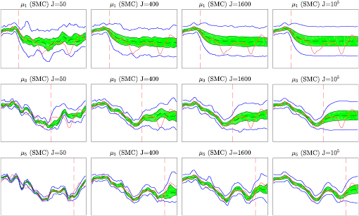
Figure 4. Percentiles of the posteriors  's (
's ( ) obtained via SMC with (from left to right) J = 50, 400, 1600, 105. Solid red line corresponds to the graph of the true log-permeability
  . Vertical dotted line indicates the location of the true front
  .
.
Download figure:
Standard image High-resolution imageIn order to quantify the level of approximation obtained with SMC with the aforementioned selections of parameters, we compute the  -relative errors of the mean and variance with respect to the posterior measure approximated with the highly-resolved SMC computed as described in the preceding subsection. More precisely, let us define

where  and
and  are the
  -posterior mean and variance characterized via SMC with large J from (53) and (54). In the previous expressions
  and
and  are the sample mean and variance defined in (53) obtained from the ensemble
  computed via SMC for the choices of small J stated above and with the aforementioned selections of tunable parameters. In addition, we consider the estimator of the true log-permeability defined by the ensemble mean
  and thus we monitor the corresponding
  -relative error defined by

Quantities  ,
,  and
and  are random variables that depend on the initial ensemble of particles that we generate from the prior
  . We thus report these quantities (for each
  ) averaged over 15 experiments corresponding to different selections of the initial ensemble of particles. In figure 5 we display
  (top),
  (middle) and
  (bottom) for (from left to right)
  as a function of the aforementioned selections of ensemble size J. For brevity we omit the results for
  as they display similar behaviour. The total computational cost of computing the full sequence of posteriors (i.e.
  from (51)) is shown in figure 6 (left). We reiterate that this cost is expressed in terms of the number of evaluations of the 5th forward map
  .
.

Figure 5. SMC approximations. Top and middle: relative errors of mean (top) and variance (middle) of the posteriors  , (from left to right)
  , obtained with SMC with different choices of small (log) ensemble size
  and tunable (SMC) parameters Jthresh and
  . Bottom: relative errors with respect to the truth
  of the ensemble mean.
Download figure:
Standard image High-resolution image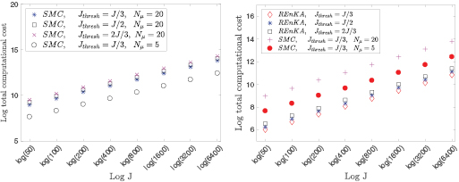
Figure 6. Total computational cost in terms of  -forward model evaluations. Left: total computational cost obtained via SMC with different choices of
  and Jthresh. Right: comparison of total computational cost obtained via REnKA with different choices of
  against the cost of SMC with different selection of tunable parameters
  and Jthresh.
Download figure:
Standard image High-resolution imageWhile the numerical analysis of the convergence of the SMC sampler is beyond the scope of this work, the results presented in this section are aimed at understanding the level of accuracy of SMC with relatively small number of particles and for a selection of tunable parameters which may enable the use of this method in more practical scenarios. From these results it is clear that the selections of Jthresh have no substantial effect on the accuracy of the scheme in terms of approximating the mean and variance of each posterior. Similarly, the computational cost with respect to our selections of Jthresh does not seem to vary significantly. It is evident that the main effect in terms of accuracy is the choice of MCMC steps (i.e. parameter  ). Indeed, note that the error obtained with
  is considerably larger than the one with
  although the computational cost of the former is one quarter of the computational cost of the latter. We conclude that even though decreasing
  can offer computational affordability, it is detrimental to the approximation properties of the scheme. This comes as no surprise as it is well known that the mutation step that involves running MCMC is crucial for the accuracy of any SMC methodology.
The behavior of the SMC sampler with respect to the number of particles J is as expected. On the one hand, an increase in J corresponds to a decrease in the error with respect to the mean and variance. On the other hand, the computational cost,  , increases with J. Note that there is a clear linear relationship between these two variables which is, in turn, obvious from (51) provided that qn is invariant with respect to J. Indeed, for the cases considered here, the number of intermediate tempering distributions (not reported) computed at each observation time, is invariant with respect to our choices of J. This is somewhat an expected outcome since our choice of Jtresh in (45) is always a fraction of J. It is also worth mentioning that the effect of J is less noticeable when we look at the error with respect to the truth. At each observation time, we notice that the
  seems to converge to a nonzero value as J increases. Note that convergence to the truth is not ensured due to the limited number of measurements inverted and the potential lack of identifiability of the log-permeability.
The results reported in this subsection suggest that achieving a reduction in the computational cost by reducing  has a severe detrimental effect in the accuracy of the SMC sampler with small number of particles. In addition, Jthresh does not seem to have a substantial effect in either the accuracy or computational cost. Clearly, we are only then limited to the number of particles J to control the computational cost of the sampler without severely compromising accuracy of the approximate posteriors.
4. Approximating the posteriors via a regularizing ensemble Kalman algorithm
In the previous section we have demonstrated, by means of numerical examples, that an accurate approximation of the Bayesian posteriors via the state-of-the art SMC samplers results in a very high computational cost; hence it is unfeasible for practical applications such as the 2D resin injection in RTM introduced in section 1. In this section we propose a regularizing ensemble Kalman algorithm (REnKA) that aims at providing an accurate approximation of the sequence of Bayesian posteriors at a much lower computational cost. In section 4.1 we introduce REnKA as a Gaussian approximation from the SMC sampler of [22] discussed in the preceding section. The proposed REnKA in the context of existing ensemble Kalman methods is discussed in section 4.2. A numerical investigation of the convergence properties of REnKA is reported in section 4.3.
For the subsequent development of the proposed scheme, we extend the domain of definition of the sequence of forward maps  introduced in (22). More specifically, we assume
  where
where  is a Hilbert space such that
 ![$X=C[0, x^{*}]\hookrightarrow\mathcal{X}$](https://content.cld.iop.org/journals/0266-5611/34/10/105002/revision2/ipaad1ccieqn377.gif) (compactly). We denote by
(compactly). We denote by  and
and  the inner products in
  and
and  , respectively. In addition, we define
  with inner product denoted by
  .
.
4.1. Motivation for REnKA
Motivated by the SMC tempering approach described in the previous section, we now propose an ensemble Kalman algorithm whose aim is to approximate  by a sequence of Gaussian measures
  which are, in turn, characterised by a set of particles with equal weights. Suppose that, at time t = tn we have an ensemble
  of J samples from a Gaussian measure
  that approximates
  , and a prescribed tempering parameter
  . We may then solve (45) for the new
  and define the regularization parameter
  in (48). We now wish to make a transition from
  to a Gaussian measure
  that approximates
  . To this end, it is convenient to define the augmented variable

and note that, in terms of this variable, we may rewrite (50) as

where  and I is the identity operator. One can see that by reformulating the inverse problem in terms of the augmented variable, the resulting forward map (i.e. H) acting on this variable is linear.
From (57) we define the following augmented particles

and construct the empirical Gaussian measure:

where
and
The Gaussian measure  is used to approximate the measure, denoted by
  , that arises from pushing forward
  under (57). By using this Gaussian approximation of
  , we then provide a Bayesian formulation of the inverse problem given by (58). More specifically, we wish to compute
  given
given  and the data from (58). A formal application of Bayes theorem yields

Moreover, from (60) and the linearity of the forward map H (on the augmented variable), it follows by standard arguments [26] that

where

Let us then note that Cn,r−1 in (62) can be written as

where
and
Informally, we use the block structure of (66) and define  , the approximation of
  , as the marginal measure of
  given by

where

Although the measure (70) is fully characterised by its mean and covariance, for the subsequent tempering step we need a particle approximation of  . We can obtain those particles by updating the current set of particles
  via the formula

where

Indeed, under the standard assumption that the noise  is independent from
  , it can be shown by the standard arguments in Kalman-based methods (see for example [7]) that
Expression (72) leads to an iterative (regularised) ensemble Kalman-based algorithm, summarized in algorithm 1, for which the proposed selection of the regularisation parameter  is based on the tempering approach discussed in section 3.2. While this selection of
  ensures a smooth transition between the measures
  and
and  in SMC, we conjecture that a similar effect should be observed between the corresponding Gaussian approximations computed via the REnKA scheme, thereby leading to stable and reasonably accurate approximations of the posteriors computed via small number of samples. Our conjecture will be verified via numerical experiments in section 4.3.
Algorithm 1. Regularizing ensemble Kalman algorithm (REnKA).
Let  be the initial ensemble of J particles. be the initial ensemble of J particles. |
| Define the tunable parameter Jthresh. |
for  do do |
Set r = 0 and  ; ; |
while  do do |
 |
Compute the nth likelihood (29)  for for  . . |
(this implies computing  needed below). needed below). |
Compute the tempering parameter  : : |
if ![$\min\nolimits_{\phi\in (\phi_{n, r-1}, 1]}{\rm ESS}_{n, r}(\phi)>J_{\rm thresh}$](https://content.cld.iop.org/journals/0266-5611/34/10/105002/revision2/ipaad1ccieqn422.gif) then then |
set  . . |
| else |
compute  such that such that  using a using a |
bisection algorithm on ![$(\phi_{n, r-1}, 1]$](https://content.cld.iop.org/journals/0266-5611/34/10/105002/revision2/ipaad1ccieqn426.gif) . . |
| end if |
Construct  , ,  defined by expressions (67) and (68). defined by expressions (67) and (68). |
| Update each ensemble member: |
for  do do |
 |
| where |
 |
with  |
| end for |
| end while |
Set  . Approximate . Approximate  with with  |
| end for |
Remark 4.1. Note that the key assumption for the proposed scheme is the Gaussian approximation of  provided by (64). It is clear that the measure
  is, as a rule, non-Gaussian and the aforementioned assumption will result in a methodology that will, in general, not converge to the posteriors
  as the ensemble size
  . Nevertheless, we will show via numerical examples that this approximation provides reasonably accurate estimates using only a small number of particles.
It is not difficult to see that the main computational cost of REnKA, in terms of the cost of evaluating the forward model at the final observation time, is given by

where, as before, gn denotes the computational cost of evaluating the  -forward map. As we will demonstrate via numerical experiments, for the moving boundary problem of section 2.1, REnKA offers a computationally affordable and thus practical approach to approximate the solution to the Bayesian inverse problem that arises from RTM.
It is important to mention that, at a given observation time tn and iteration level r, the value of  may be zero to machine precision. In this case, the tempering parameter
  is not be computable, via a bisection scheme on
 ![$(\phi_{n, r-1}, 1]$](https://content.cld.iop.org/journals/0266-5611/34/10/105002/revision2/ipaad1ccieqn443.gif) , as stated in algorithm 1. This computational issue is more likely to arise at the early iterations of the scheme for which the value of
, as stated in algorithm 1. This computational issue is more likely to arise at the early iterations of the scheme for which the value of  is not sufficiently close to one. This can be overcome, for example, by simply adapting the bisection algorithm in order to first compute a
  such that
  . If
. If ![$\min\nolimits_{\phi\in (\phi_{n, r-1}, \phi_{\ast}]}{\rm ESS}_{n, r}(\phi)>J_{\rm thresh}$](https://content.cld.iop.org/journals/0266-5611/34/10/105002/revision2/ipaad1ccieqn447.gif) we then set
we then set  ; otherwise, we find
  by solving (45) via a bisection algorithm on
 ![$(\phi_{n, r-1}, \phi_{\ast}]$](https://content.cld.iop.org/journals/0266-5611/34/10/105002/revision2/ipaad1ccieqn450.gif) . For the numerical experiments reported in the present work, zero values to machine precision for
. For the numerical experiments reported in the present work, zero values to machine precision for  were only encountered where a large number of measurements were inverted in the 2D setting of section 5.
4.2. REnKA in the context of existing ensemble Kalman methods for inverse problems
Ensemble Kalman methods for inverse/calibration problems have been widely used in the last decades [15, 20]. More recently, using iterative Kalman methods with a regularization parameter (e.g.  in (75)) have been proposed for a wide class of applications. In particular, the proposed REnKA scheme can be related to the recently developed regularizing ensemble Kalman method introduced in [19] for solving classical (deterministic) inverse problems. More precisely, algorithm 1 is nothing but a sequential version of the iterative scheme presented in [19] except for the selection of the regularization parameter
  . While in the present work we have motivated algorithm 1 from the SMC framework, the algorithm in [19] was obtained as an ensemble approximation of the regularizing Levenberg–Marquardt scheme initially developed in [16] for solving ill-posed inverse problems. In the context of the proposed work, REnKA aims at providing a derivative-free approximation to the solution of

in a stable (regularized) fashion. The regularization parameter in [19] was selected according to the discrepancy principle in order to regularize the inverse problem posed by (77). In contrast, the present work uses the adaptive tempering approach of [22] for the selection of this regularization parameter in the context of SMC. It is clear that tempering can be understood as a regularization to the Bayesian inverse problem; the effect of  is to flatten out the posterior and allow for a more controlled/regularized transition between the sequence of measures. Other works highlighting the connection between ensemble Kalman methods and SMC approaches include [40, 44, 45]. In addition, by noticing from (48) that, for each
  ,
,  , the proposed REnKA can be also understood as a sequential version of the ensemble smoother with multiple data assimilation proposed by [12]. However, it is important to reiterate that the adaptive selection of
  proposed here is inherited from the SMC approach of [22]. This selection differs substantially from the strategy proposed in [12] for which the number of intermediate tempering distributions qn is fixed and selected a priori.
4.3. Numerical approximating the posterior with REnKA
In this subsection we report the results from applying REnKA proposed in section 4.1 for the approximation of the sequence of posteriors  that we introduced in the framework of section 3.4. The algorithm is applied with the same selection of ensemble sizes (J = 50, 100, 200, 400, 800, 1600, 3200, 6400) that we use for the SMC sampler of section 3.5. In addition, we consider three choices of the tunable parameter Jthresh (
 ). In figure 7 we display the percentiles of the log-permeability posteriors
  ,
,  and
and  obtained with REnKA, for a fixed set of initial ensembles, and for some of these choices of J. For comparison purposes we include the fully resolved posterior (via SMC) in the right column of figure 7. We can clearly observe that the approximations provided by REnKA improves as the ensemble size J increases. More importantly, we can note that the uncertainty band defined by these percentiles provided better approximations than those from SMC with the same number of particles (see figure 4).
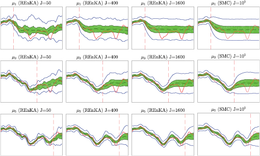
Figure 7. Percentiles of the posteriors  ,
,  , and
, and  obtained via REnKA with (from left to right)
  and SMC (right column) with J = 105. Solid red line corresponds to the graph of the true log-permeability
  . Vertical dotted line indicates the location of the true front
  .
.
Download figure:
Standard image High-resolution imageWe quantify the level of accuracy of REnKA with respect to the Benchmark defined by the highly-resolved SMC sampler reported in section 3.4.2. In figure 8 we display  (top),
  (middle) and
  (bottom) for (from left to right)
  computed with the REnKA samples with various ensemble sizes J. Similar results (not shown) are obtained for
  . The total computational cost (
 from (76)) of computing the full sequence of posteriors is shown in figure 6 (right). In figures 8 and 6 (right) we also include some of the results obtained with the SMC samplers with the same choice of small number of particles discussed in section 3.5. These results speak for themselves; given a small number of particles, REnKA provides a much more accurate approximation of the posterior measures than SMC. For example, note that for the final measure
  , REnKA (applied with
  ) with an ensemble of J = 200 particles yields
  ,
,  at a computational cost of
 -forward model evaluations. In order to obtain a similar level of accuracy (
 ,
,  ), we need to apply the SMC sampler (say with
  , and
, and  ) with J = 6400 particles for which the computational cost is approximately
 -forward model evaluations.

Figure 8. Top and middle: relative errors of mean (top) and variance (middle) of the posteriors  , (from left to right) n = 1,3, 5, obtained via REnKA with different choices of (log) ensemble size
  and tunable parameter Jthresh. Bottom: relative errors of the ensemble mean obtained via REnKA with respect to the truth
  .
.
Download figure:
Standard image High-resolution imageThe results above not only demonstrate that, when a small number of particles is used, the performance (accuracy versus computational cost) of REnKA outperforms SMC, but also these results show that REnKA is robust for reasonable selections of the tunable parameter Jthresh. Similar to SMC, this parameter determines the number of tempering distributions at each observation time and thus has an impact on the computational cost of the scheme. It is also important to remark that even though the relative errors of REnKA with respect to the mean and variance decrease as the ensemble size increases, these errors seem to converge to a non-zero value thereby indicating that REnKA does not provide an asymptotic convergence to the posterior measures as  . Nevertheless, our results clearly showcase the advantages of REnKA for approximating these measures in an accurate and efficient fashion for a limited and realistic computational cost.
Having numerical evidence from section 4.3 that REnKA is a robust and computationally feasible approach for addressing the Bayesian inverse problem defined in section 2, in section S1 of the supplementary material SupMat we provide further practical insights in the Bayesian inverse problem for the 1D case studied earlier. In particular, we study effect of (i) number/type of measurements, (ii) number of observation times and (iii) observational noise level, on the sequence of Bayesian posteriors that result from approximating, via REnKA, the Bayesian inverse problem in the 1D case.
5. Bayesian inversion in 2D RTM
In this section we apply REnKA for the Bayesian inversion of the 2D moving boundary problem described by (1)–(9). In contrast to the 1D case, the numerical solution of the 2D moving boundary problem is much more computationally intensive. Therefore, the application of a fully Bayesian methodology such as the SMC sampler considered in section 3 is impractical for an online computation of the Bayesian posteriors in the 2D case. In this subsection, we exploit the capabilities of REnKA for providing an accurate yet computationally tractable approach for inferring preform (log) permeability alongside with its uncertainty.
5.1. Formulation of the 2D Bayesian inverse problem
Let us consider now the 2D moving boundary problem introduced (1)–(9) from section 1. We recall that we are interested in the inference of the log-permeability  given noisy measurements of the pressure field
  from M sensors located at points
  collected at a discrete observation times
  . In addition, we wish to invert observations of the front location, or alternatively from the moving domain
  that can be potentially obtained from CCT cameras such as in [32, 49]. While in the 1D case we can trivially define observations of the (single point) front, in 2D the front
  is a curve which defines the moving domain
  . Therefore, rather than dealing with measurements of the front
  itself we may assume pointwise measurements of
  via its characteristic function defined by

More precisely, we define observations of the form  , where
  is an array of points for which the characteristic function of
  is observed. In practice this array should be considered dense when a high resolution camera is used for capturing the moving domain. Note that this mathematical description of front measurements is suitable as it enables its direct comparison with observations from digitalized images and also with the discrete formulation of (2)–(9) via the control volume finite element method (CV/FEM) in which the front location is characterized in terms of the filling factor (see details in [38]) rather than using a parameterization of
  .
.
For specified (known) pI, p0,  ,
,  , φ, the solution of (2)–(9) induces a map
 ![$u=\log{\kappa} \to [\,p(x, t), D(t)]$](https://content.cld.iop.org/journals/0266-5611/34/10/105002/revision2/ipaad1ccieqn506.gif) which enables us to define the sequence of forward maps
which enables us to define the sequence of forward maps  by means of

To our best knowledge, uniqueness, existence and regularity theory for problem (2)–(9) with non constant  is an open problem for d > 1 (see a related discussion in [38]). However, for the present work we assume that the following condition holds.
Assumption 1. The sequence of forward maps  (
( ) are continuous.
We now follow the same formulation of the Bayesian inverse problem as the one we described in section 2.2. At each observation time t = tn, we collect noisy measurements of the front location  as well as pressure measurements from sensors
  . We assume that observations
 ![$ \newcommand{\Ga}{\Upsilon} y_{n}=[y_{n}^{\Ga}, y_{p}]^{T}$](https://content.cld.iop.org/journals/0266-5611/34/10/105002/revision2/ipaad1ccieqn513.gif) are related to the unknown via expressions (25) -(26) with
are related to the unknown via expressions (25) -(26) with  defined in (79). As before, both measurements of
  (via its characteristic function) and pressures are assumed to be uncorrelated in time and independent from each other. Furthermore, we consider Gaussian priors
  with a covariance operator
  that arises from the Whittle–Matern correlation function defined in (27). The assumption of continuity of the forward maps as well as the fact that
  ensures existence of the sequence of posterior measures
  given by theorem 2.5 with the same definition of the likelihood functions introduced in (29). In the following section we use REnKA to to compute an ensemble approximation of
  .
.
5.2. 2D numerical experiments
In this subsection we apply REnKA for the solution of the 2D Bayesian inverse problem defined in the previous subsection. The forward model described by (1)–(9) is solved numerically with the MATLAB code developed in [38] and available from https://github.com/parkmh/MATCVFEM. This code is based on the interface-tracking control volume finite element method (CV/FEM) [3, 17, 48]. For experiments of this subsection, we consider the following fixed values:

Samples from  are generated via KL parametrization as described in section 2.2.1 with parameters
  ,
,  , l = 0.1 and
  for all
  . Some draws from the prior are displayed in figure 9 (middle row). The log-permeability field is plotted in figure 9 (top-left) is a random draw from the prior that we use as the truth
  for the present experiments.
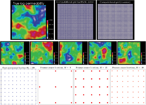
Figure 9. Top-left: true log permeability (![$\log[{\rm m}^{2}]$](https://content.cld.iop.org/journals/0266-5611/34/10/105002/revision2/ipaad1ccieqn527.gif) ). Top-middle: computational domain for the generation of synthetic data. Top-right: computational domain for the inversion (via REnKA). Middle row: random draws from the Gaussian prior
). Top-middle: computational domain for the generation of synthetic data. Top-right: computational domain for the inversion (via REnKA). Middle row: random draws from the Gaussian prior  (
(![$\log[{\rm m}^{2}]$](https://content.cld.iop.org/journals/0266-5611/34/10/105002/revision2/ipaad1ccieqn529.gif) ); bottom row: measurement configuration for the moving front
); bottom row: measurement configuration for the moving front  (left); pressure measurement configuration with (from left to right) M = 9, M = 25 and M = 49 sensors.
Download figure:
Standard image High-resolution imageWe use one dense configuration of  measurement locations
  for the observation of the moving domain given in terms of (78); these locations are displayed in figure 9 (bottom-left). We have selected a large number of measurements locations assuming that the moving domain can be densely observed with high-resolution cameras or dielectric sensors. In addition, we consider three possible configurations of M = 9, M = 25 and M = 49 pressure sensors
  , whose locations are shown in the left-middle to right panels of figure 9 (bottom). The summary of measurement configurations that we investigate are summarised below:

where ✓ (resp.  ) indicates whether the moving domain D(tn) has been observed via (78).
We use the true log-permeability to numerically solve the forward model (1)–(9) via the CV/FEM code described above. Then, for each of these measurement configurations, synthetic data with a realistic choice of 2.5% Gaussian noise are generated in a similar manner to the one described in section 3.4.1. In order to avoid inverse crimes, synthetic data are computed on a finer grid than the one we use for the Bayesian inversion via REnKA. These are shown in the middle and right panels of figure 9 (top). Snapshots of the true pressure field  at the initial time t0 and observation times
  (in seconds) are displayed in figure 10 alongside with the corresponding true moving domain
  .
.
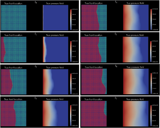
Figure 10. Snap shots of the true pressure field (Pa) and the true moving domain  for the initial time t0 and the observation times
  (s).
(s).
Download figure:
Standard image High-resolution imageFor the application of REnKA we use a fixed number of J = 150 with tunable parameter  . For clarity of the notation, in the expression for the ensemble mean and variance (54), we then omit the index J as appropriate. The following numerical investigations are focused on the following quantities defined at each observation time tn (
 ):
):
- (A)a measure of the uncertainty provided by the-norm of the ensemble variance relative to the prior, i.e.
- (B)a normalized-error with respect to the truth defined by


We report quantities in (A) and (B) averaged over 15 experiments corresponding to different selection of the initial ensemble from the prior. The motivation for using the normalized  -error instead of the relative error as defined in (56) is discussed in section S2 of the supplementary material SupMat.
For the configuration with ( ) the ensemble mean and (log) variance of each posterior
  approximated with REnKA are displayed in figure 11. We note that as more observations (in time) are assimilated, the ensemble mean better captures the spatial features of the truth while the (variance) uncertainty is reduced in the region of the true moving domain
  . In figure 12 we show the ensemble mean and (log) variance of the final time posterior
  approximated via REnKA for different choices of the number of pressure sensors and with the inversion of the moving domain (✓). Note that the pure inversion of the moving domain (i.e. M = 0 pressure sensors) results in an informative measure of the log-permeability. It is clear that the accuracy in the estimation of the log-permeability improves with the number of pressure sensors.

Figure 11. Ensemble mean and variance of  obtained via REnKA at each observation time. The true moving boundary has been included at each of these observation times.
Download figure:
Standard image High-resolution image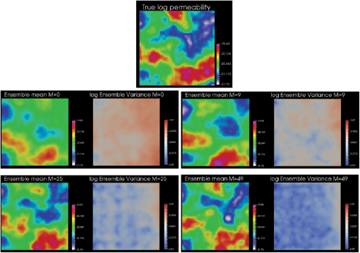
Figure 12. Top: true-log permeability. Bottom: ensemble mean and variance of  obtained via REnKA at the final observation time t7.
Download figure:
Standard image High-resolution imageFrom the plot of  displayed in figure 13 (left), we note that, at the latest observation times (
 ), there is a clear improvement in the accuracy with increasing the number of pressure locations. Similar to the 1D case, we also observe that the benefit of inverting measurements from the moving domain is only noticeable when the number of pressure sensors is relatively small (M = 9). This configuration of sensors is more realistic in practical settings. It is also worth noticing that, at the earliest observation times (
 ) when the front has not reached most pressure sensors, inverting measurements from the moving domain provides additional information of the log-permeability to the one provided only by pressure measurements.
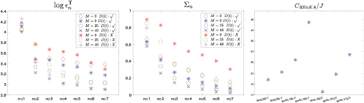
Figure 13. Performance of REnKA (J = 150) for the the approximation of the posterior measures  with measurement configurations from (80). Left:
  from (82). Middle: relative norm of the variance
  (81). Right: scalable (with respect to J) computational cost of REnKA.
Download figure:
Standard image High-resolution image
As more observations (in time) are assimilated, the reduction of the uncertainty in terms of the ensemble variance can be observed from the plot of  displayed in figure 13 (middle). From this plot we also note that the variance decreases as we increase the number of pressure sensors. The added value of measurements from the moving domain is also quite substantial and more noticeable for a small number of pressure sensors. In fact, note that smaller uncertainty has been achieved by inverting only the front (M = 0) compared to the inversion of only pressure data from M = 9 sensors. Here we also find that, at the earliest observation times, the additional inversion of measurements of the moving domain results in further reductions of the uncertainty in comparison to the inversion of only pressure data. While this investigation was conducted with a realistic choice of measurement noise (2.5%), further studies should be conducted to understand the effect of the noise level on the uncertainty estimates of log-permeability in the 2D case.
Finally, the computational cost (see expression (76)) of approximating the sequence of posteriors  via REnKA is displayed in figure 13 (right). This cost is expressed in terms of the number of
  forward model evaluations which, in turn, correspond to solving the moving boundary problem from t = 0 to the last observation time t7. Furthermore, this cost has been normalised by the number of particles J used in REnKA. This normalisation enables us to provide a rough estimate of the scalable (with respect to J) computational cost of the REnKA (76) if each evaluation of the forward map (see step 2(b) in algorithm 1) is conducted in parallel. As discussed in section 3.3, increasing the number of measurements results in more tempering distributions (i.e. iterations) in the REnKA scheme. Therefore the computational cost increases with the number of measurements. However, for a realistic choice of pressure sensors M = 9, we note that cost of inverting measurements of both front location and pressure sensor results (in average) in a scalable cost of 21 iterations. Since the number of particles that we use for REnKA is relatively low (J = 150), such scalability with respect to the number of particles is reasonable with a high-end computer cluster and can be achieved within a few minutes.
6. Summary and conclusions
In this work we studied the Bayesian inverse problem that arises from inferring physical properties in a setting for porous media flow with a moving boundary. Our investigation is focused on the inference of log-permeability from measurements of pressure and observation of the (moving) domain occupied by resin during the resin injection stage of RTM relevant to the fabrication of composite materials. We adopted the infinite-dimensional Bayesian approach to inverse problems where the aim is to characterise, at each observation time, the posteriors that arise from conditioning the log-permeability on pressure/front measurements. The simplicity of the 1D RTM model enabled us to show existence of the Bayesian posteriors in the aforementioned infinite-dimensional setting. These posteriors were then probed numerically with the dimension-independent SMC sampler for inverse problems from [22]. Our numerical experiments indicated that very large number of particles were needed to accurately approximate the Bayesian posteriors. This resulted in a high computational cost unfeasible for practical RTM settings.
In order to reduce computational cost of Bayesian inversions for practical RTM settings, we proposed a regularising ensemble Kalman algorithm (REnKA) that we motivated from the adaptive tempering SMC sampler of [22]. The proposed REnKA is based on Gaussian approximations of the sequence of Bayesian posteriors and thus, in general, asymptotic convergence of posterior expectations cannot be ensured. Nevertheless, our numerical results demonstrated that REnKA is robust with respect to tuneable parameters and provides reasonably accurate estimates of the posterior mean and variance with a computational cost affordable for practical RTM processes.
While measurements have been widely used with ad-hoc approaches to estimate permeability of preform in RTM, to the best of our knowledge, this work constitutes the first investigation that uses a Bayesian inverse modeling framework for random moving boundary problems. From the numerical investigations that we conducted some conclusions and recommendations can be made with relevant implications to practical RTM settings. In particular, our synthetic experiments indicated that, when a small number of sensors (5 sensors in 1D and 9 sensors in 2D) are used to measure pressure, observing the front/moving domain can substantially reduce the uncertainty (variance) of the estimates of the log-permeability. This is particularly relevant in real experiments when the number of pressure sensors are usually limited. However, when the inversion is conducted with only measurements of the moving front, the reconstruction of the main spatial features of the true permeability are not recovered accurately.
Our results also display the benefit of the proposed sequential approach in updating our knowledge of the log-permeability as soon as measurements become available. Indeed, inverting measurements of pressure and front frequently in time, enabled us to reduce the uncertainty in the log-permeability. While the reduction of the uncertainty is mainly achieved within the region occupied by the resin at a given time, a decrease in the uncertainty (with respect to the prior) can also be observed in an unfilled region close to the front. Such a reduction of this uncertainty via the Bayesian posteriors can be valuable for decision-making purposes with the aim of an active control of RTM in real time. Further, we note that the proposed sequential approach is also beneficial in terms of obtaining more accurate estimates with respect to the truth than those obtained if the algorithm is modified to (iteratively) invert data all-at-once. More precisely, we conducted numerical experiments where we inverted, simultaneously, the entire set of data collected during a given time window for given synthetic experiment. Our results (not displayed) suggest that the sequential approach outperforms the all-at-once approach, producing estimates with smaller errors with respect to the truth and smaller variances of the log-permeability.
Finally, our numerical investigations show that the observation noise in pressure measurements and front location have a substantial effect on the estimates of log-permeability and its uncertainties. Indeed, it comes as no surprise that more accurate measurements (e.g.  ) result in estimates of log-permeability concentrated around the truth. Again, giving the limitation of deploying many pressure sensors within a real RTM scenario, it is then essential to use high precision pressure sensors to achieve enough confidence in the posterior uncertainties of the inferred permeability.
Although the context of this work is related to the resin injection in RTM processes, the Bayesian framework at the core of the proposed methodology, and the corresponding Gaussian approximations emerged from the proposed REnKA are generic, flexible, and thus transferable to a wide class of inverse problems constrained by PDEs with moving boundaries.
Acknowledgments
This work was supported by the Engineering and Physical Sciences Research Council [grant number EP/K031430/1]. The authors are very grateful to Mikhail Matveev for useful discussions. MI wishes to thank Nikolas Kantas for helpful discussions on the computational aspects and implementation of SMC.
Appendix A.: Proof of theorem 2.2
For the proof of theorem 2.2 we consider the dimensionless version of (19) and (20) that we derive in the following subsection.
A.1. Dimensional analysis
Let us consider the following change to dimensionless variables:

where tf is a reference time and u0 is a reference (constant) log-permeability. For simplicity we choose
which enable us to transform (19) and (20) into


where, with a slight abuse in the notation, the variables p, u,  , x and t are now the dimensionless variables. Similarly, the dimensionless filling time (21) is given by

Let us note from (A.2) and (18) that

Recall that  is the collection of observation times with
  and
and  are the pressure measurement locations (
 ). We now prove two technical lemmas which are needed for the proof of theorem 2.2.
A.2. Technical lemmas
For all ![$ \newcommand{\e}{{\rm e}} u\in X\equiv C[0, x^{\ast}]$](https://content.cld.iop.org/journals/0266-5611/34/10/105002/revision2/ipaad1ccieqn567.gif) , we define the norm
, we define the norm
and denote by  the corresponding solutions of the dimensionless moving boundary problem (A.2) and (A.3). Similarly, the filling time given by (A.4) is denoted by
  .
.
Lemma A.1. For all ![$ \newcommand{\e}{{\rm e}} u\in X\equiv C[0, x^{\ast}]$](https://content.cld.iop.org/journals/0266-5611/34/10/105002/revision2/ipaad1ccieqn570.gif) , there exists a constant
, there exists a constant  such that

for all ![$t, \hat{t}\in [t_{1}, \tau^{\ast, u}]$](https://content.cld.iop.org/journals/0266-5611/34/10/105002/revision2/ipaad1ccieqn572.gif) . The constant
. The constant  may depend only on
  and
and  .
.
Proof. Let  and
and ![$t\in [t_{1}, \tau^{\ast, u}]$](https://content.cld.iop.org/journals/0266-5611/34/10/105002/revision2/ipaad1ccieqn577.gif) . From (A.5) and (18) it is clear that
. From (A.5) and (18) it is clear that  is increasing and satisfies
  . Therefore,

Then, from (A.5) we have that

which implies

Similarly, note that

and so

for all ![$t\in[t_{1}, \tau^{*, u}]$](https://content.cld.iop.org/journals/0266-5611/34/10/105002/revision2/ipaad1ccieqn580.gif) . The Mean Value theorem combined with (A.11) yields (A.6). □
. The Mean Value theorem combined with (A.11) yields (A.6). □
Lemma A.2. For all  , there exists a constant
  , such that


for all ![$t\in [t_{1}, \min\{\tau^{\ast, u}, \tau^{\ast, v}\}]$](https://content.cld.iop.org/journals/0266-5611/34/10/105002/revision2/ipaad1ccieqn583.gif) and all
and all  . Moreover,

The constant  may depend only on
  and
and  .
.
Proof. From the mean value theorem it is not difficult to see that

where
It is also not difficult to see that

From (A.15) and (A.16), and the fact that  , we have

From (A.11) we get

Therefore
We recall that  and use Gronwall's inequality to conclude that
From (A.4) we see that

which we combine with (A.19) to obtain

where

Hence, (A.11) is proved.
Let us now consider the case  and
and  , then

for all ![$t\in [0, \min\{\tau^{*, u}, \tau^{*, v}\}]$](https://content.cld.iop.org/journals/0266-5611/34/10/105002/revision2/ipaad1ccieqn592.gif) . Assume now that
. Assume now that  ,
,  , and let us note that

Therefore, from (A.3), (A.11), (A.24), (A.15), (A.17) and (A.21), we find
Consider now the case  ,
,  . From (A.3) and (A.24) that
  . Therefore,
Since  (recall
  ) and
) and  , it then follows from (A.16), (A.11) and (A.21) that
Hence, (A.12) is proved.
Finally, from (A.4) and (A.15), it is easy to see that

We combine (A.21), (A.23), (A.25)–(A.27) and then (A.12)–(A.14) follows with
□
A.3. Proof of theorem 2.2
Given  fixed, we first establish continuity of the following map
  . Let
. Let  and without loss of generality assume that
  . Note that

Since  , the previous expression reduces to

We observe that we can write

Then by lemmas A.1 and A.2, we obtain

for all ![$t\in [\tau^{*, v}, \tau^{*, u}]$](https://content.cld.iop.org/journals/0266-5611/34/10/105002/revision2/ipaad1ccieqn606.gif) . We combine (A.31) with (A.28) and use lemma A.1 again to obtain
. We combine (A.31) with (A.28) and use lemma A.1 again to obtain

for all  which establishes the continuity of
  and, in particular, of
  for all
  .
.
Similarly, we now prove the continuity of  . We note that

From (A.3) it follows
for all ![$t\in [\tau^{\ast, v}, \tau^{\ast, u}]$](https://content.cld.iop.org/journals/0266-5611/34/10/105002/revision2/ipaad1ccieqn612.gif) . Using (A.31) as well as similar arguments to the ones used before, we obtain
. Using (A.31) as well as similar arguments to the ones used before, we obtain
We use (A.35), (A.11) and the fact that  to rewrite (A.34) as follows
From similar arguments it is easy to see that
We use (A.36) and (A.37) and lemma A.2 to conclude that

which proves the continuity of  for all
  . The continuity of
  then follows. □
Appendix B. SMC sampler and pcn-MCMC algorithm
In algorithm 2 we display the pcn-MCMC method that we use for the mutation step in the SMC sampler of [22] discussed in section 3.2 and summarized in algorithm 3 below.
Algorithm 2. pcn-MCMC to generate samples from a  -invariant Markov kernel.
Select  and an integer and an integer  . . |
for  do do |
Initialize  |
while  do do |
| (1) pcN proposal. Propose uprop from |
 |
(2) Set  with probability with probability  and and  with probability with probability  , where , where |
 |
| with ln,r defined in (46) |
(3)  |
| end while |
| end for |
Algorithm 3. SMC algorithm for high-dimensional inverse problems.
Let  be the initial ensemble of J particles. be the initial ensemble of J particles. |
Define the tunable parameters Jthresh and  . . |
for  do do |
Set r = 0 and  |
While  do do |
 |
Compute the nth likelihood (29)  (for (for  ) ) |
Compute the tempering parameter  : : |
if  then then |
set  . . |
| else |
compute  such that such that  |
using a bisection algorithm on ![$(\phi_{n, r-1}, 1]$](https://content.cld.iop.org/journals/0266-5611/34/10/105002/revision2/ipaad1ccieqn643.gif) . . |
| end if |
Computing weights from expression (44) ![$ \newcommand{\e}{{\rm e}} W_{n, r}^{(\,j)}\equiv \mathcal{W}_{n, r-1}^{(\,j)}[\phi_{n, r}]$](https://content.cld.iop.org/journals/0266-5611/34/10/105002/revision2/ipaad1ccieqn644.gif) |
Resample. Let  , , |
Set  and and  |
Mutation. Sample  via algorithm 2. via algorithm 2. |
| end while |
Set  . Approximate . Approximate  by by  |
| end for |
Appendix C. Numerical implementation of the 1D forward model
In this section we discuss the key aspects of the numerical implementation of the dimensionless version of the 1D RTM forward model derived in appendix A.1.
Note that Fu defined in (18) can we written as

where
is the Heaviside function. In order to approximate (A.2) and (A.3), we discretize the domain ![$[0, 1]$](https://content.cld.iop.org/journals/0266-5611/34/10/105002/revision2/ipaad1ccieqn652.gif) with S subintervals with end points defined by
with S subintervals with end points defined by ![$x_{s+1/2}=[1/2+s]\Delta x$](https://content.cld.iop.org/journals/0266-5611/34/10/105002/revision2/ipaad1ccieqn653.gif)
 , where
  and the centers of the cells are
  . Let us consider a piecewise constant approximation of the unknown u defined on the centers of the cells, i.e.
where  . Therefore, (C.1) can be approximated by

where we have replaced  with its smooth approximation
  (with r = 300) [6].
We consider a temporal domain ![$[0, 0.4]$](https://content.cld.iop.org/journals/0266-5611/34/10/105002/revision2/ipaad1ccieqn660.gif) discretized with K points
discretized with K points  , where
  . An implicit backward Euler scheme applied to the dimensionless version of (16) yields

where  . For the approximation of (C.3), we use (C.2). The solution of the resulting nonlinear equation is implemented in MATLAB by means of the routine fzero. Once
  is computed, we evaluate the pressure field from

at the mesh points xs+1/2 defined earlier.