

Abstract
We derive a general formula for the inertia tensor of a rigid body consisting of three particles with which students can learn basic properties of the inertia tensor without calculus. The inertia-tensor operator is constructed by employing the Dirac's bra-ket notation to obtain the inertia tensor in an arbitrary frame of reference covariantly. The principal axes and moments of inertia are computed when the axis of rotation passes the center of mass. The formulas are expressed in terms of the relative displacements of particles that are determined by introducing Lagrange's undetermined multipliers. This is a heuristic example analogous to the addition of a gauge-fixing term to the Lagrangian density in gauge field theories. We confirm that the principal moments satisfy the perpendicular-axis theorem of planar lamina. Two special cases are considered as pedagogical examples. One is a water-molecule-like system in which a particle is placed on the vertical bisector of two identical particles. The other is the case in which the center of mass coincides with the incenter of the triangle whose vertices are placed at the particles. The principal moment of the latter example about the normal axis is remarkably simple and proportional to the product 'abc' of the three relative distances. We expect that this new formula can be used in actual laboratory classes for general physics or undergraduate classical mechanics.
Export citation and abstract BibTeX RIS

Original content from this work may be used under the terms of the Creative Commons Attribution 4.0 licence. Any further distribution of this work must maintain attribution to the author(s) and the title of the work, journal citation and DOI.
1. Introduction
The inertia tensor of a rigid body as well as the center of mass (CM) is a fundamental physical quantity involving the rotational motion in classical mechanics. One of the most elementary ingredients that students must learn regarding the inertia tensor is that there are three principal axes along which the angular momentum becomes parallel to the angular velocity. These three principal axes form a natural choice of orthogonal basis vectors for the Cartesian coordinates that span the three-dimensional Euclidean space. A principal moment of inertia is the corresponding value for the moment of inertia when the rigid body rotates about a principal axis. In mathematical point of view, the inertia tensor is a real and symmetric matrix that is always diagonalizable. Thus the eigenvalues, the principal moments of inertia, are real and the eigenvectors, the principal axes, are orthogonal. The principal axes, the eigenvectors for normal modes, and the eigenstates for a Hermitian operator in quantum mechanics have all a common mathematical structure. In the same manner, the principal moments of inertia, normal frequencies, and the energy eigenvalues for the Hamiltonian have a common mathematical feature. Hence, the mathematical techniques of linear algebra that students acquire from the computation of inertia tensor can be strong backgrounds for their future learning of the coupled oscillators, normal modes of string vibration, and their quantum mechanical extensions to Hermitian matrices.
Our motivation of this work is to provide a systematic treatment of inertia-tensor calculation by employing the languages commonly used in rather advanced levels like quantum mechanics and quantum field theory. For example, we employ Dirac's bra-ket notation [1] to define the inertia-tensor operator that has been presented in reference [2] based on the covariant approach to a symmetric tensor that can be found, for example, in reference [3]. Dirac's bra-ket notation is commonly used in mathematics because the notation greatly simplifies the computation and allows one to avoid cumbersome expressions to write. In physics textbooks, the bra-ket notation appears only in the advanced level of quantum mechanics at the point the expressions are quite involved. Basically, the ket corresponds to a column vector and a bra corresponds to a row vector. In matrix representation, the scalar product of two vectors can be expressed as the matrix product of a row vector and a column vector. Thus we can make a compact expression to represent the scalar product of two vectors in terms of bra-ket notation. In addition, a rank-2 Cartesian tensor, which carries two vector indices, such as the inertia tensor can also be expressed as the projection of an operator onto a bra and a ket. The reason is that the matrix element of that tensor can be expressed as the scalar product of a basis ket and another basis bra multiplied by some operator sandwiched by the bra and ket. This factorization makes the coordinate dependence into the basis bra and ket leaving the operator independent of the coordinate system. The explicit expression of each matrix element for the inertia tensor is a linear combination of the Kronecker delta and direct products of the position vectors of constituent particles weighted by corresponding masses. Thus the corresponding inertia-tensor operator can be constructed as the linear combination of the identity operator and the direct products of the bras and kets corresponding to the position vectors for the constituent particles. Complications due to the coordinate dependence can be avoided if one constructs an invariant expression by employing the bra-ket notation.
Once the inertia-tensor operator for a rigid body is constructed, one can always read off the inertia tensor from the inertia-tensor operator covariantly by multiplying the bra and ket of unit basis vectors of a given Cartesian coordinates. After obtaining the covariant expression for the inertia tensor, we fully keep the covariant expression without substituting explicit values for the tensor or vector components. The coefficients of the tensor expansion are all expressed in terms of the invariant quantities that are masses and the scalar products of available displacement vectors. The covariant analysis is a common tool in particle physics in which all of the physical observables are expressed as tensors or vectors that transform covariantly as basis changes. In this approach, the expression for a physical observable is expressed in terms of the maximal number of invariant quantities such as scalar products and the remaining frame-dependent components are kept implicitly. Keeping the covariance simplifies the calculation greatly and one can make use of the formula in any frame of reference.
As a model system to apply our tools to study the rigid-body motion, we select an arbitrary three-body system. In usual textbooks like reference [4] on classical mechanics, the inertia tensors for two-body systems and specific rigid bodies like rods, plates, discs, cubes, and spheres are considered. However, students are not frequently exposed to a three-body system except for very simple systems like three particles forming the three vertices of an equilateral triangle. Nevertheless, the rigid body consisting of three particles is particularly interesting for the following reasons: (i) one does not require calculus to evaluate the CM and the inertia tensor, (ii) the coplanar nature of the CM with the constituents greatly simplifies the rigid body mechanics. For example, a principal axis is always normal to the plane of the rigid body and the principal moment of inertia along that normal axis is the sum of the other two principal moments of inertia because of this coplanar nature. Because one out of three principal axes is automatically determined, the diagonalization process to find the other two principal axes is relatively simple. Because of these reasons listed above, a general three-body system contains rich heuristic contents to study without too much difficult computations.
In our analysis, we need to express the position vectors in terms of those for the CM and the relative displacements of the particles. The relation results in a set of indeterminate linear equations whose transformation matrix has vanishing determinant. We introduce a generalized version of the Lagrange undetermined multiplier that is analogous to the addition of a gauge-fixing term to the Lagrangian density in gauge field theories [5]. If we employ a physical gauge, the number of the physical degrees of freedom is less than that is required to have the Green's function exist. However, by introducing a gauge-fixing term in the Lagrangian density function, one can restore the missing degrees of freedom to have the Green's function calculable. The gauge-fixing term is the gauge condition multiplied by a Lagrange undetermined multiplier. Suppose that we employ a class of Lorenz gauge in which ∂μ
Aμ
= 0, where Aμ
is the gauge field, ∂μ
is the four-derivative, and μ is the four-vector index that runs from 0 to 3. For example, if one employs the Rξ
gauge that is a generalized Lorenz gauge, then one still has the constraint equation ∂μ
Aμ
= 0 and one has the freedom to add the gauge-fixing term  to the Lagrangian density
  of the gauge field Aμ
, where 1/ξ is the Lagrange undetermined multiplier. After introducing this additional term, the missing degrees of freedom of the gauge field are restored and the Green's function (propagator of the gauge field) can be computed. However, the undetermined multiplier 1/ξ (gauge-fixing parameter) does not contribute to physical observables such as an invariant amplitude or cross sections. This is guaranteed by the fundamental principle, gauge invariance. The disappearance of the undetermined multiplier 1/ξ in a gauge-invariant physical observable is not required by the substitution of the constraint equation. Theoretical particle physicists resort to this gauge invariance as a very useful tool to confirm the validity of their computation by checking that their final result is free of the undetermined multiplier such as 1/ξ. Just like the gauge-fixing parameter that decouples from the theory after evaluating a physical observable, the undetermined multipliers in our calculation also disappear in the final result.
of the gauge field Aμ
, where 1/ξ is the Lagrange undetermined multiplier. After introducing this additional term, the missing degrees of freedom of the gauge field are restored and the Green's function (propagator of the gauge field) can be computed. However, the undetermined multiplier 1/ξ (gauge-fixing parameter) does not contribute to physical observables such as an invariant amplitude or cross sections. This is guaranteed by the fundamental principle, gauge invariance. The disappearance of the undetermined multiplier 1/ξ in a gauge-invariant physical observable is not required by the substitution of the constraint equation. Theoretical particle physicists resort to this gauge invariance as a very useful tool to confirm the validity of their computation by checking that their final result is free of the undetermined multiplier such as 1/ξ. Just like the gauge-fixing parameter that decouples from the theory after evaluating a physical observable, the undetermined multipliers in our calculation also disappear in the final result.
This paper is organized as follows: in section 2, we list the definitions of various physical variables that we frequently use in the remainder of this paper. Section 3 contains an exhaustive set of invariant and covariant physical variables to describe the inertia tensor of the three-body system that are determined by employing Lagrange undetermined multipliers. The computation of the inertia tensor of the three-body system is given in section 4 which also provides results for the covariant expressions for the principal axes and invariant expressions for the principal moments of inertia. A couple of pedagogical examples of three-body system are considered in section 5 which is followed by discussions in section 6.
2. Definitions
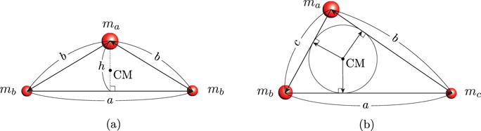
Let us consider a rigid-body system consisting of three particles of mass ma , mb , and mc placed at points A, B, and C whose position vectors are A , B , and C , respectively, as shown in figure 1. We denote the total mass of the system by M = ma + mb + mc . The CM of the system is at

We attach a superscript ⋆ to represent a vector in the CM frame such that

where  is the position vector for the CM. In the CM frame, the three lever-arm vectors
  ,
,  , and
, and  from the CM are coplanar:

If the rigid body is rotating about an axis  with the angular velocity
  , then the rotational kinetic energy Krot of the system is given as
where Iij is the inertia tensor [6] of the system determined as

Here, δij
is the Kronecker delta and ωi
, Ai
, Bi
, and Ci
are components of
ω
,
A
,
B
, and
C
, respectively, with respect to the unit Cartesian bases  's. Note that we have used the following identity in the second line in equation (4):

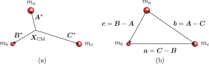
Figure 1. (a) The lever-arm vectors A ⋆, B ⋆, and C ⋆ from the CM, X CM, to three particles of mass ma , mb , and mc , respectively. (b) The side vectors a , b , and c defined in equation (17 ), where A , B , and C are the position vectors of the points A, B, and C.
Download figure:
Standard image High-resolution imageIn a similar manner, the angular momentum  about an axis passing the CM and parallel to the unit vector
  by an angular velocity
  of the three-body system can be expressed as
where we have made use of the BAC-CAB rule
A
× (
B
×
C
) =
B
(
A
⋅
C
) −
C
(
A
⋅
B
). Here,  is the inertia tensor Iij
in equation (5) with the replacements
A
→
A
⋆,
B
→
B
⋆, and
C
→
C
⋆. According to the second equality in equation (7), the angular momentum
L
⋆ is parallel to
ω
if
ω
is normal to the plane
is the inertia tensor Iij
in equation (5) with the replacements
A
→
A
⋆,
B
→
B
⋆, and
C
→
C
⋆. According to the second equality in equation (7), the angular momentum
L
⋆ is parallel to
ω
if
ω
is normal to the plane  on which the triangle is lying.
Because the inertia tensor Iij
is real and symmetric, it is always diagonalizable. The three eigenvalues of the inertia tensor are called the principal moments of inertia. The three corresponding eigenvectors are called the principal axes that are orthogonal and construct a natural set of the basis vectors spanning the three-dimensional space. As a result, if a rigid body rotates about a principal axis  with the angular velocity
  , then the angular momentum is parallel to that axis:

It is apparent that the normal vector  to the triangle plane
  is always a principal axis for this three-body system.
As is given in reference [2], we employ the bra-ket notation [1] to express the inertia tensor. The ket |
U
⟩ represents the vector
U
and the corresponding bra ⟨
U
| represents its dual vector. In matrix representation, the ket |
U
⟩ corresponds to the column-vector representation  and the bra ⟨
U
| corresponds to the row-vector representation
and the bra ⟨
U
| corresponds to the row-vector representation  for the vector
U
. The transformation between the bra and ket for a single vector is equivalent to the transpose in matrix representation. The scalar product between two Euclidean vectors
U
and
V
is commutative and can be expressed in bra-ket representation as
for the vector
U
. The transformation between the bra and ket for a single vector is equivalent to the transpose in matrix representation. The scalar product between two Euclidean vectors
U
and
V
is commutative and can be expressed in bra-ket representation as

The ith Cartesian component Ui
of a vector
U
can be expressed as the scalar product  , where
  is the unit vector along the ith Cartesian axis. In bra-ket notation, it can be expressed as

An operator O acts on any ket and bra to map it into another ket and bra, respectively. Then the identity operator 1 can be defined as an operator that maps any ket (or bra) to itself. The identity operator corresponds to the identity matrix  in matrix representation. Hence, the property of the identity operator ⟨
U
|1|
V
⟩ = ⟨
U
|
V
⟩ can be used to express the matrix element of the identity matrix by making use of the bra-ket notation as
in matrix representation. Hence, the property of the identity operator ⟨
U
|1|
V
⟩ = ⟨
U
|
V
⟩ can be used to express the matrix element of the identity matrix by making use of the bra-ket notation as

We can construct the operator | U ⟩⟨ V | whose matrix elements in the Cartesian coordinates are given by the product Ui Vj :

Hence, the operator |
U
⟩⟨
V
| corresponds to the direct product  in matrix representation. As a result, the inertia tensor Iij
defined in equation (5) can be understood as the matrix element of an operator in the basis set
in matrix representation. As a result, the inertia tensor Iij
defined in equation (5) can be understood as the matrix element of an operator in the basis set  . While Iij
varies covariantly depending on the basis choice, the operator representation has a merit in that it is independent of the basis set.
. While Iij
varies covariantly depending on the basis choice, the operator representation has a merit in that it is independent of the basis set.
By employing the bra-ket notation, we can express the inertia tensor in equation (5) as
where I is the inertia-tensor operator defined by

Note that the inertia-tensor operator I is of invariant representation: as well as the coefficients, the operator form is independent of the coordinate system. Once we project out the inertia tensor Iij from the inertia-tensor operator I, then the expression acquires covariant quantities such as Ai Aj : a covariant quantity is dependent on the coordinate system but the transformation from a coordinate system to another is systematically related. Therefore, once we know the inertia-tensor operator I, we can obtain the inertia tensor in an arbitrary frame by projection covariantly as shown in equation (13). We keep the complete covariant structure of the inertia tensor until the last step of computation without substituting explicit components of Euclidean vectors A , B , and C .
Huygens–Steiner parallel-axis theorem [7] can be employed to express the inertia tensor as

where  is the inertia tensor at the CM and
  is the ith Cartesian component of
X
CM. The corresponding inertia-tensor operator is given by
is the ith Cartesian component of
X
CM. The corresponding inertia-tensor operator is given by

We define the displacements  ,
,  , and
, and  that are independent of the frame of reference as
where a , b , and c are side vectors as shown in figure 1(b). It is manifest that the sum of the three side vectors vanishes

Unlike the position vectors A , B and C , which depend on the reference point, the lever-arm vectors and side vectors can be considered as invariant under coordinate transformation or basis choice in the sense that they are determined just from the geometric property of the triangle.
3. Lagrange multipliers and invariants
The lever-arm vectors A ⋆, B ⋆, and C ⋆ defined in equation (2) depend not only on the positions of the particles but also on the masses of the particles, while the side vectors a , b , and c defined in equation (17) depend only on the positions of the particles. We want to separate the contributions of the positions and the masses in the lever-arm vectors by expressing A ⋆, B ⋆, and C ⋆ in terms of the side vectors a , b , and c and the masses of the particles ma , mb , and mc .
As are defined in equation (17), the lever-arm vectors and the side vectors are connected by the conversion matrix Λ as

According to equation (18), only two of the three side vectors
a
,
b
, and
c
are linearly independent so that Λ is not invertible: ![$\mathcal{D}et[{\Lambda}]=0$](https://content.cld.iop.org/journals/0143-0807/42/5/055016/revision3/ejpabf8c6ieqn33.gif) and Λ−1 does not exist. This is a kind of indeterminate linear equation that has multiple solutions. We introduce a regularization procedure that makes this indeterminate equation solvable like a regular problem involving invertible transformation matrix. The regularization requires a modification of the problem from the original form that can be achieved by introducing a parameter called a regulator. The temporarily introduced regulator should be removed in a consistent manner at the end of the regularization procedure to restore the original problem. The specific way of regularization is called the regularization scheme and the final result must be independent of the specific scheme.
and Λ−1 does not exist. This is a kind of indeterminate linear equation that has multiple solutions. We introduce a regularization procedure that makes this indeterminate equation solvable like a regular problem involving invertible transformation matrix. The regularization requires a modification of the problem from the original form that can be achieved by introducing a parameter called a regulator. The temporarily introduced regulator should be removed in a consistent manner at the end of the regularization procedure to restore the original problem. The specific way of regularization is called the regularization scheme and the final result must be independent of the specific scheme.
The method of Lagrange undetermined multiplier can be interpreted as a regularization scheme to solve such an indeterminate linear equation whose regulator is the Lagrange multiplier. Let us consider a mechanical system with n generalized coordinates q1, ⋯, qn with a constraint equation f(q1, ⋯, qn ) = 0. Because of the constraint f(q1, ⋯, qn ) = 0, we cannot vary all of the coordinates qi independently to find the constraint equation for the extremum of the action, which is the Euler-Lagrange equation of motion. The independence of all of the coordinates can be restored by adding an additional term λf(q1, ⋯, qn ) to the Lagrangian and keeping from applying the constraint, f(q1, ⋯, qn ) = 0. The free parameter λ is called the Lagrange undetermined multiplier. The regularized equation is

where L is the original Lagrangian of the system. Once one derives n independent equations of motion, one can impose the constraint f(q1, ⋯, qn ) = 0 that results in a system of n + 1 equations for n coordinates and an undetermined multiplier λ. Then the coordinates and the undetermined multipliers are all determined by solving the whole system of equations. After solving the system of equations, the multiplier λ is identified to be the constraint force that restricts the mechanical system to satisfy the constraint equation f(q1, ⋯, qn ) = 0. While the Lagrange undetermined multiplier is originally applied to Lagrangian mechanics, the essential characteristic of the multiplier is to make a dependent variable in the original system of equations temporarily an independent variable. Therefore, the regularization of a system of indeterminate linear equations can also be made by generalizing the method of Lagrange multiplier developed in Lagrangian mechanics. In Lagrangian mechanics, the regularization is implemented at the Lagrangian level by adding a vanishing contribution multiplied by a multiplier to the Lagrangian because the equation of motion must satisfy the least-action principle. In contrast, when regularizing a set of linear indeterminate equations, we can directly modify the equations by adding vanishing contributions multiplied by Lagrange multipliers as is shown in reference [8].
In order to solve equation (19), we introduce three Lagrange undetermined multipliers [9–12] λ1, λ2, and λ3 as regulators. Our regularization scheme is to multiply these Lagrange multipliers λ1, λ2, and λ3 to the vanishing expression ma A ⋆ + mb B ⋆ + mc C ⋆ in equation (3) and add them to the original equation (19) for a , b , and c , respectively. As a result, the regularized equation modified by the Lagrange multipliers is

where the regularized transformation matrix Λ'(λ1, λ2, λ3) is given by

It is manifest that the sum of the three regularized equations is

While a + b + c = 0 and ma A ⋆ + mb B ⋆ + mc C ⋆ = 0 are independent conditions in the original problem, the regularization makes the values for a + b + c and ma A ⋆ + mb B ⋆ + mc C ⋆ correlated as is given in equation (23 ). Therefore, the requirement of a + b + c = 0 is effectively the same as the substitution of ma A ⋆ + mb B ⋆ + mc C ⋆ = 0. It is the result from the choice we made in equation (22 ) to regularize the indeterminate equations. According to the constraint equation (3), the modification does not affect the equation at all. However, if we do not impose the constraint in equation (3) temporarily, then all of the three linear equations become linearly independent. Thus the regularized transformation matrix Λ'(λ1, λ2, λ3) in equation (22 ) is invertible and we can solve the regularized linear equation (21 ) by multiplying the inverse matrix Λ'−1(λ1, λ2, λ3). This is equivalent to the situation that one does not apply the constraint equations until the Euler-Lagrange equation of motion is obtained when employing Lagrange undetermined multipliers in Lagrangian mechanics. In the aspect that an additional degree of freedom is created by the introduction of a single multiplier, the parameters λi behave like the Lagrange undetermined multiplier. Because there is only one linearly dependent variable due to the presence of a single constraint equation (3), we must introduce at least one independent multiplier. Thus two of the three parameters are actually redundant. We, however, allow all three parameters in order to keep the cyclic symmetry of the expression in the intermediate step. By multiplying the inverse matrix Λ'−1(λ1, λ2, λ3) to equation (21 ), we find that
where the determinant ![$\mathcal{D}\equiv \mathcal{D}et[{{\Lambda}}^{\prime }({\lambda }_{1},{\lambda }_{2},{\lambda }_{3})]$](https://content.cld.iop.org/journals/0143-0807/42/5/055016/revision3/ejpabf8c6ieqn34.gif) is given by
is given by

Note that the existence of Λ'−1(λ1, λ2, λ3) implies that all of the three rows of both Λ'(λ1, λ2, λ3) and Λ'−1(λ1, λ2, λ3) are linearly independent. This is true only if the sum of the Lagrange multipliers λ1 + λ2 + λ3 is not vanishing according to equation (25 ). The expressions in equation (24 ) are expressed in terms of linearly dependent vectors a , b , and c according to equation (18). We shall find that the Lagrange multipliers λi in equation (24 ) disappear completely as soon as we express these vectors in terms of a pair of linearly independent side vectors instead of all side vectors a , b , and c . To do that, we require the condition a + b + c = 0 or, equivalently, ma A ⋆ + mb B ⋆ + mc C ⋆ = 0. As a result, the expressions for the lever-arm vectors take the compact forms:

It is remarkable that every λi dependence in equation (24 ) completely cancel analytically because the numerator has the same factor (λ1 + λ2 + λ3) that every denominator has. Thus A ⋆, B ⋆, and C ⋆ in equation (26) are all independent of the Lagrange multipliers. This complete decoupling of the Lagrange undetermined multipliers indicates that the regularization does not restrict the multipliers to have certain values. All of the multipliers are actually allowed except for combinations that satisfy λ1 + λ2 + λ3 = 0. The fundamental reason for this decoupling is originating from the fact that the regularization we have employed has not changed the equation at all. The presence of the Lagrange multipliers allowed the transformation matrix invertible. However, the addition of a new degree of freedom in the regularized transformation matrix in equation (22 ) does not affect the dimensions in which all of the relevant vectors are residing.
The complete disappearance of the Lagrange undetermined multipliers λi is a special feature of the Lagrange multiplier as the regulator of a set of indeterminate linear equations in (19). This is in strong contrast to that employed in Lagrangian mechanics. Note that the regularized equation of motion in equation (20 ) contains the constraint function as a partial derivative λ∂f/∂qi . Hence, the λ dependence (λ∂f/∂qi ) in the regularized equation of motion does not disappear in general even after imposing the constraint equation f(q1, ⋯, qn ) = 0. Therefore, the Lagrange multiplier λ is not a fictitious parameter but a physical variable that indeed interferes the system and has its own physical meaning as the constraint force. However, our Lagrange multiplier does not interfere the system but allows only the inverse linear transformation by providing a missing degree of freedom in a given transformation matrix. Thus the parameters appear only in the intermediate result or in a representation expressed in terms of linearly dependent vectors or expressions. This does not mean that the parameters are vanishing because they must not be vanishing simultaneously according to equation (25 ).
Such a complete decoupling of the Lagrange multiplier in a physical problem happens in the gauge-fixing parameter ξ that is employed to add an additional term to the Lagrangian density  of the gauge field. In quantum electrodynamics, a photon has only two independent degrees of freedom while it is described by the four-vector gauge field
  with the gauge-invariant Lagrangian density

where the summation over repeated Greek indices μ and ν is assumed from 0 to 3. Here, Fμν is the electromagnetic field-strength tensor defined by

Note that  ,
,  ,
,  ,
,  ,
,  , and c is the speed of light. The antisymmetric tensor Fμν
has 6 independent components consisting of the electric and magnetic fields, which are invariant under the gauge transformation with an arbitrary scalar field χ:
, and c is the speed of light. The antisymmetric tensor Fμν
has 6 independent components consisting of the electric and magnetic fields, which are invariant under the gauge transformation with an arbitrary scalar field χ:

The equation of motion for the gauge field Aμ
can be obtained by finding the condition for the extremum of the action corresponding to the Lagrangian density (27
) under the variation of all of the four components of the gauge field Aμ
independently. The equation of motion for the gauge field is equivalent to the Maxwell's equations. Then, the Fourier transformation  in the momentum space is a solution for a system of indeterminate linear equations whose transformation matrix is singular like equation (19). This is the result caused by the mismatch between the degrees of freedom of a photon and the corresponding gauge field Aμ
. One can add a gauge-fixing term
in the momentum space is a solution for a system of indeterminate linear equations whose transformation matrix is singular like equation (19). This is the result caused by the mismatch between the degrees of freedom of a photon and the corresponding gauge field Aμ
. One can add a gauge-fixing term ![$-\frac{1}{2\xi }{[f({A}^{\mu })]}^{2}$](https://content.cld.iop.org/journals/0143-0807/42/5/055016/revision3/ejpabf8c6ieqn43.gif) in the Lagrangian density to regularize this equation to make it invertible. The gauge-fixing term is indeed the product of the Lagrange undetermined multiplier −1/(2ξ) and the vanishing expression
in the Lagrangian density to regularize this equation to make it invertible. The gauge-fixing term is indeed the product of the Lagrange undetermined multiplier −1/(2ξ) and the vanishing expression ![${[f({A}^{\mu })]}^{2}$](https://content.cld.iop.org/journals/0143-0807/42/5/055016/revision3/ejpabf8c6ieqn44.gif) corresponding to the gauge condition f(Aμ
) = 0, where the constraint function f(Aμ
) depends on a specific gauge. Because every component of the gauge field must be treated to be independent in deriving the Euler-Lagrange equation, the Lagrange undetermined multiplier must keep the independence of the four components of Aμ
. This is the reason why the gauge-fixing term
corresponding to the gauge condition f(Aμ
) = 0, where the constraint function f(Aμ
) depends on a specific gauge. Because every component of the gauge field must be treated to be independent in deriving the Euler-Lagrange equation, the Lagrange undetermined multiplier must keep the independence of the four components of Aμ
. This is the reason why the gauge-fixing term ![$-\frac{1}{2\xi }{[f({A}^{\mu })]}^{2}$](https://content.cld.iop.org/journals/0143-0807/42/5/055016/revision3/ejpabf8c6ieqn45.gif) is proportional to the square of f(Aμ
). This is distinguished from the classical implementation of the undetermined multiplier that is employed only when making dependent coordinates released to be independent. Therefore, the gauge-dependent contribution decouples as soon as we require the gauge condition f(Aμ
) = 0. Here, the gauge condition f(Aμ
) = 0 and the gauge-fixing parameter ξ fill the missing degrees of freedom for the transformation matrix of the indeterminate linear equation for
is proportional to the square of f(Aμ
). This is distinguished from the classical implementation of the undetermined multiplier that is employed only when making dependent coordinates released to be independent. Therefore, the gauge-dependent contribution decouples as soon as we require the gauge condition f(Aμ
) = 0. Here, the gauge condition f(Aμ
) = 0 and the gauge-fixing parameter ξ fill the missing degrees of freedom for the transformation matrix of the indeterminate linear equation for  . Comparing the case of the electromagnetism with that of the three-body inertia tensor, one can see that the side vectors
a
,
b
, and
c
are analogous to the components of the field-strength tensor Fμν
that are invariant under gauge transformation, the position vectors
A
,
B
, and
C
are analogous to the components of the gauge field Aμ
in an arbitrary gauge, the lever-arm vectors
A
⋆,
B
⋆, and
C
⋆ are analogous to those components in a specific gauge with the gauge condition, ma
A
⋆ + mb
B
⋆ + mc
C
⋆ = 0 is analogous to a specific gauge condition, and λi
is analogous to the gauge-fixing parameter. In this case, the above constraint equation can be considered to be analogous to the Coulomb gauge conditions, A0 = ϕ = 0 and
. Comparing the case of the electromagnetism with that of the three-body inertia tensor, one can see that the side vectors
a
,
b
, and
c
are analogous to the components of the field-strength tensor Fμν
that are invariant under gauge transformation, the position vectors
A
,
B
, and
C
are analogous to the components of the gauge field Aμ
in an arbitrary gauge, the lever-arm vectors
A
⋆,
B
⋆, and
C
⋆ are analogous to those components in a specific gauge with the gauge condition, ma
A
⋆ + mb
B
⋆ + mc
C
⋆ = 0 is analogous to a specific gauge condition, and λi
is analogous to the gauge-fixing parameter. In this case, the above constraint equation can be considered to be analogous to the Coulomb gauge conditions, A0 = ϕ = 0 and  ⋅
⋅  = 0. In both cases, only physical degrees of freedom survive after imposing the conditions.
According to equation (17) and figure 1(b), the angle between
a
and
b
is π − ∠C and so on. Here, we denote the internal angle of the triangle at vertex C by ∠C, and similarly for ∠A and ∠B. The scalar products of unit vectors  ,
,  , and
, and  parallel to
a
,
b
, and
c
, respectively, are
parallel to
a
,
b
, and
c
, respectively, are
where a = | a |, b = | b |, and c = | c | are side lengths of a triangle with vertices A, B, and C. By making use of equations (26) and (30), we can express the scalar products of lever-arm vectors in terms of side lengths and masses as
where μij = mi mj /(mi + mj ) is the reduced mass of a two-body system.
4. Inertia tensor
Now all of the lever-arm vectors are completely determined in terms of the side vectors that are independent of the Lagrange undetermined multipliers λi
. Thus any quantities that derive from the side vectors are also independent of the parameter λi
. As a result, the inertia tensor  that depends only on the lever-arm vectors is completely independent of the parameter λi
in a similar manner as the gauge-invariant quantities such as invariant amplitude and cross sections that do not depend on the gauge-fixing parameter. We have reached the stage in which every expression is uniquely defined without ambiguity once we express any physical observables involving the inertia tensor
that depends only on the lever-arm vectors is completely independent of the parameter λi
in a similar manner as the gauge-invariant quantities such as invariant amplitude and cross sections that do not depend on the gauge-fixing parameter. We have reached the stage in which every expression is uniquely defined without ambiguity once we express any physical observables involving the inertia tensor  in terms of the side vectors. According to laws of cosines in equation (30), any scalar products are expressed in terms of a2, b2, and c2 that are linearly independent. This is manifest from the expressions in equation (31
). We shall find that the principal axes are all expressed as linear combinations of the side vectors. The coefficients of the expansion and the principal moments of inertia are all expressed in terms of the exhaustive set of invariant quantities ma
, mb
, mc
, a2, b2, and c2. This is analogous to the disappearance of the gauge-fixing parameter in any physical observable that is invariant under gauge transformation.
in terms of the side vectors. According to laws of cosines in equation (30), any scalar products are expressed in terms of a2, b2, and c2 that are linearly independent. This is manifest from the expressions in equation (31
). We shall find that the principal axes are all expressed as linear combinations of the side vectors. The coefficients of the expansion and the principal moments of inertia are all expressed in terms of the exhaustive set of invariant quantities ma
, mb
, mc
, a2, b2, and c2. This is analogous to the disappearance of the gauge-fixing parameter in any physical observable that is invariant under gauge transformation.
The inertia tensor for arbitrary masses and length parameters can be computed by making use of the inertia-tensor operator in equation (16) covariantly. In this section, we compute the principal axes and moments of inertia of the three-body system. As we have discussed in equation (8), the normal vector  to the plane
  , on which the triangle is lying, is always a principal axis. Therefore, the set of the three principal axes can be constructed as
  . Because they are orthogonal,
  are orthogonal unit vectors spanning
  .
.
If the axis of rotation passes the CM, then the moment of inertia about  is
is

Because
A
⋆,
B
⋆, and
C
⋆ are coplanar on  and
and  is perpendicular to
  , the coefficient of
  must be the same as that for 1:

where  is the two-dimensional identity operator on the plane
  . We choose the cyclic orthonormal basis vectors as
Then  and
and

where
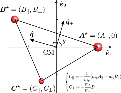
Figure 2. The lever-arm vectors of the three particles in the frame where
A
⋆ is along the x axis. The principal axes  and
and  can be obtained by rotating
  and
and  , respectively, by an angle θ defined in equation (39
).
, respectively, by an angle θ defined in equation (39
).
Download figure:
Standard image High-resolution imageHere, X∥ and X⊥ are the components of X ⋆ that are parallel and perpendicular to A ⋆, respectively, as shown in figure 2. We can replace the components of C ⋆ with those of A ⋆ and B ⋆ by making use of the CM condition C ⋆ = −(ma A ⋆ + mb B ⋆)/mc .
The inertia-tensor operator becomes most compact if we choose the principal axes to be the basis vectors  , where

The principal axes  can be obtained by rotating
  as
as

where the angle θ is

The principal moments of inertia are now determined as
The rotationally invariant quantities involving A ⋆, B ⋆, and C ⋆ are
Substituting equation (41) into equation (36
) and applying equation (31
), we express the principal moments  ,
,  , and
, and  in equation (40) in terms of only the masses and side lengths:
To the best of our knowledge, the formulas in equation (42) are new. Here, Källén function λ(a2, b2, c2) is defined by

Note that Källén function λ(a2, b2, c2) is related to the area S of a triangle with side lengths a, b, and c as

where sin ∠A, sin ∠B, and sin ∠C are determined from the identities in equation (30) as
It is manifest that the expressions in equation (42) satisfy the perpendicular-axis theorem of planar lamina [13],

5. Examples
In this section, we present two pedagogical examples with which we demonstrate how our results given in the previous section apply.
5.1. Water-molecule-like system
We consider a triatomic molecule in which an atom of mass ma
is on the vertical bisector of the other identical atoms with mb
= mc
by a perpendicular distance h. The three atoms form the vertices of an isosceles triangle which is a triangle whose two side lengths are equal. For instance, water molecule (H2O) corresponds to this system as shown in figure 3(a). Then b can be expressed in terms of a and h as  . Substituting
  and mc
= mb
into equation (42), we obtain the corresponding principal moments of inertia as
and mc
= mb
into equation (42), we obtain the corresponding principal moments of inertia as
Note that  is either
  or
or  . The results in equation (47) agree with the expression in the solution of the problem 1(b) in reference [14] where μ in reference [14] is the total mass of the system M = ma
+ 2mb
.
. The results in equation (47) agree with the expression in the solution of the problem 1(b) in reference [14] where μ in reference [14] is the total mass of the system M = ma
+ 2mb
.
Figure 3. (a) A water-molecule-like system in which A is on the vertical bisector of the identical particles B and C (mb = mc ) with the perpendicular distance h. (b) A system whose CM coincides with the incenter of the triangle ABC to have a:b:c = ma :mb :mc .
Download figure:
Standard image High-resolution image
5.2. When CM coincides with the incenter
The next example has the property that the side length opposite to a particle is proportional to its mass:

Manifestly, the following ratios are all equal:

Under the condition in equation (48), the CM in equation (1) coincides with the incenter X in of the triangle as shown in figure 3(b),

In geometry, the incenter of a triangle is the point at which the three angle bisectors meet. And there is a circle centered at the incenter that inscribes the three sides of the triangle simultaneously. In this case, the principal moments in equation (42) can be expressed as
To the best of our knowledge, the formulas in equation (51 ) are new.
6. Discussions
We have derived a general formula for the inertia tensor of a rigid body consisting of arbitrary three bodies. The invariant form of the inertia-tensor operator was constructed by making use of Dirac's bra-ket notation as reference [2]. While the bra-ket notation is widely employed in many mathematics textbooks, the notation appears in physics textbooks only from the level of quantum mechanics or higher. However, as we have seen in the derivation, the notation is particularly useful in classical mechanics, too. We argue that a lot of experiences can be made regarding the bra-ket notation when undergraduate students study the inertia tensor in classical mechanics as we presented in this paper. The covariant form of the inertia tensor can be found by projecting the basis kets from the inertia-tensor operator. The principal moments of inertia are obtained in terms of the invariant quantities, masses and side lengths. In addition to the vector  normal to the plane
  on which the three particles are lying, there are two more principal axes. The covariant formulas for the three principal axes are expressed in terms of the lever-arm vectors whose coefficients are the invariant quantities listed above. The normal vector
  is always a principal axis. The other two principal axes
  on the plane
  are obtained in equation (38
). The general expressions for the principal moments of inertia are given in equation (42) for
are obtained in equation (38
). The general expressions for the principal moments of inertia are given in equation (42) for  and
and  . The expressions for
  involve the Källén function λ(a2, b2, c2) which is negative definite for the side lengths a, b, and c. We confirmed that the expressions in equation (42) satisfy the perpendicular-axis theorem of planar lamina,
  . To the best of our knowledge, these analytic expressions for a general three-body system are new.
In the derivation of the expressions in equation (26) for the lever-arm vectors at a CM frame, we have introduced Lagrange undetermined multipliers λi 's to solve a set of indeterminate linear equations. The complete cancellation of the parameters λi 's in equation (26) is equivalent to the disappearance of the gauge-fixing parameter, which is a Lagrange undetermined multiplier, in the evaluation of the gauge-independent physical quantity. The gauge-fixing parameter which is a Lagrange undetermined multiplier is not a physical field that does not contribute to the real world. As a result, the gauge-fixing parameter completely decouples from the expression of an observable physical quantity. While the Lagrange undetermined multiplier that appears in classical mechanics [9–12] has a certain physical meaning of the constraint force for each constraint equation, this is not always true because of a generalized version popular in the gauge field theories that we just have discussed. Such a decoupling in the quantum-field-theoretical example resembles the complete cancellation of the parameters λi 's in our case. This is the reason why we claim that the parameters λi 's are indeed Lagrange undetermined multipliers.
As pedagogical examples, we have considered two specific rigid bodies. One example is the water-molecule-like system in which a particle is on the vertical bisector of two identical particles. The corresponding principal moments of inertia listed in equation (47) derive from (42) and agree with the expressions in reference [14]. The other example has the CM that coincides with the incenter of a triangle whose vertices are at the three particles. Thus the mass of a particle is proportional to the side length opposite to itself to have the relation ma
:mb
:mc
= a:b:c. The principal moment of inertia about  of the latter example given in equation (51) is remarkably simple and proportional to the product abc. To the best of our knowledge, these compact expressions for the latter example are new.
We propose to develop a laboratory device with which students can perform experiments of three-body principal moments of inertia in actual laboratory classes for general physics or undergraduate classical mechanics. At first glance, it is almost impossible to construct a three-particle rigid body in free space with massless rods. However, if we consider the superposition properties of the inertia tensor and the moment of inertia, then it is not impossible. We can make an equipment having three empty spaces in which massive particles can be plugged. We can measure the moments of inertia I0 and Iloaded for the unloaded and loaded with the three particles, respectively. Then the moment of inertia of the three-body system can be deduced as I = Iloaded − I0. Hence, it is indeed possible to test our formulas experimentally.
Author contributions
All authors contributed equally to this work.
Acknowledgments
As members of the Korea Pragmatist Organization for Physics Education (KPOP
 ), the authors thank the remaining members of KPOP
 for useful discussions. We also thank the anonymous reviewers for providing valuable suggestions that were very helpful to improve the manuscript. This work is supported in part by the National Research Foundation of Korea (NRF) Grant funded by the Korea government (MSIT) under Contract Nos. NRF-2020R1A2C3009918 (J-HE, U-RK, DWJ, DK, and JL), NRF-2017R1E1A1A01074699 (DWJ and JL), NRF-2018R1D1A1B07047812 (DWJ), and NRF-2019R1A6A3A01096460 (U-RK). The work is also supported in part by the National Research Foundation of Korea (NRF) under the BK21 FOUR program at Korea University, Initiative for science frontiers on upcoming challenges.