
Abstract
Performing measurements of the properties of antihydrogen, the bound state of an antiproton and a positron, and comparing the results with those for ordinary hydrogen, has long been seen as a route to test some of the fundamental principles of physics. There has been much experimental progress in this direction in recent years, and antihydrogen is now routinely created and trapped and a range of exciting measurements probing the foundations of modern physics are planned or underway. In this contribution we review the techniques developed to facilitate the capture and manipulation of positrons and antiprotons, along with procedures to bring them together to create antihydrogen. Once formed, the antihydrogen has been detected by its destruction via annihilation or field ionization, and aspects of the methodologies involved are summarized. Magnetic minimum neutral atom traps have been employed to allow some of the antihydrogen created to be held for considerable periods. We describe such devices, and their implementation, along with the cusp magnetic trap used to produce the first evidence for a low-energy beam of antihydrogen. The experiments performed to date on antihydrogen are discussed, including the first observation of a resonant quantum transition and the analyses that have yielded a limit on the electrical neutrality of the anti-atom and placed crude bounds on its gravitational behaviour. Our review concludes with an outlook, including the new ELENA extension to the antiproton decelerator facility at CERN, together with summaries of how we envisage the major threads of antihydrogen physics will progress in the coming years.
Export citation and abstract BibTeX RIS

Content from this work may be used under the terms of the Creative Commons Attribution 3.0 licence. Any further distribution of this work must maintain attribution to the author(s) and the title of the work, journal citation and DOI.
1. Introduction
After nearly 40 years of work [1, 2], the field of antihydrogen ( ) spectroscopy is positioned to make the first direct precision comparisons between this antimatter atom and its matter counterpart. Since the first antiprotons (
 ) and positrons (e+) were produced for experiments, researchers have considered the topic of antihydrogen in many lights: fundamental questions about its annihilation cross section with matter, production techniques in beams and traps, and using it to make measurements exploring its nature (including hyperfine and optical spectroscopy), as well as a potential source of polarized antiprotons for high energy particle and nuclear physics experiments. Before performing any experiments, however, researchers required a source of antihydrogen, and for that, reliable sources of low-energy antiprotons. A flurry of activity in the field was ignited in the late 1980s by the construction of CERN's low energy antiproton ring (LEAR), a dedicated facility for high intensity, low energy antiprotons. Several techniques were proposed around that time for producing antihydrogen. These can be roughly divided into the energetic production of antihydrogen from antiprotons in storage rings and low energy production from antiprotons held in radio-frequency or Penning charged particle traps (see for example [3] for a concise perspective at the time). While the first successful demonstration of antihydrogen would be from relativistic beam experiments, production from trapped antiprotons has proved to be the fruitful way forward for making measurements on this exotic atomic system.
Towards the end of the LEAR programme in 1996, the first antihydrogen atoms were produced in-flight at high kinetic energies, by the PS196 experiment [4], inspired by the proposal of Munger et al [5]. This group exploited the coasting 1.2 GeV beam in LEAR and a xenon gas target to form antihydrogen via a very rare reaction in which an antiproton interaction with the (spectator) xenon nucleus created an electron–positron (e−–e+) pair. In a fraction of cases, the antiproton and positron emerged velocity-matched and bound as an antihydrogen atom. A similar result, but in accord with available theory, was also obtained by Blanford and co-workers [6] working on the E862 experiment at Fermilab, though using a hydrogen target.
Though this work confirmed expectations that antihydrogen atoms could exist, the very high kinetic energies and low production rate of the anti-atoms generated in these reactions meant that they were not suited to the type of precision studies needed to compare the properties of antihydrogen with those of hydrogen. Developments in producing cold, trapped antiprotons and positrons would lead to the next significant milestones in the study of antihydrogen.
Cold antiprotons would prove critical to the production of copious antihydrogen atoms. The last thirty or so years have seen considerable progress in the types of physics experiments that can be performed with low energy, trapped antiprotons. This field was pioneered by Gabrielse and co-workers [7, 8] in the late 1980s when antiprotons ejected from LEAR were first captured and cooled in very high-vacuum, cryogenic Penning-type traps. For a decade, such experiments (see also [9–11]) were performed more-or-less parasitically to the main LEAR programme, which typically centred upon aspects of antiproton annihilation and related medium-energy physics.
In order to nurture this growing field of research, CERN reconfigured its antiproton complex to ultimately commission the antiproton decelerator (AD) in 1999 [12, 13], a novel facility dedicated to ultra-low energy antiproton physics, with antihydrogen as a prominent research topic. The first experiments at the AD were ATHENA [14], ATRAP [15] and ASACUSA [16]. ATHENA and ATRAP had the aim of producing trapped antihydrogen for eventual spectroscopic measurements, while ASACUSA had several research programs, including the spectroscopy of exotic antiprotonic systems (most notably antiprotonic helium), the production of an antihydrogen beam, and measurements of antiproton annihilation cross sections with matter. In 2005, ATHENA disbanded, with some of its members forming ALPHA [17] with new collaborators. As of 2015, the original experiments have been joined by ACE [18], an experiment dedicated to studying the effects of antiprotons on living cells, AEgIS [19], who plan to make a measurement of the gravitational acceleration of a horizontal beam of antihydrogen, and BASE [20], who are measuring the antiproton magnetic moment to high precision. A further experiment, GBAR [21], has been approved and is expected to start running after ELENA (see section 7.1) starts operation in 2017. Our review focusses on physics with antihydrogen in particular. Recent reviews that discuss other research areas at the AD (as well as antihydrogen) include [22].
In parallel with the developments in the trapping of antiprotons, great strides were also being made in capturing and cooling low energy positrons in Penning-like traps. This was based around positron beam technology (see e.g. [23] for a review in the context of antihydrogen physics) and in particular the use of the efficient buffer gas trapping technique developed by Surko and co-workers [24, 25]. This style of sourcing on-demand, cold positrons was chosen by ATHENA (see e.g. [26]) as the primary method for producing this antihydrogen ingredient. Another method for producing positrons for production of antihydrogen involved field-ionization of positronium (Ps) produced via a converter and a radioactive positron source ( ). Such a technique [27] was used by ATRAP in their earliest work with antihydrogen. While all currently active antihydrogen experiments employ the so-called 'Surko-style' accumulator to provide low energy positrons, the development of novel sources of positrons is an area of active research with at least one proposal aimed at the use of electron linac-driven pair production, followed by positron cooling and accumulation for antihydrogen experimentation [28].
With both cold antiprotons and cold positrons in place, low energy antihydrogen followed shortly thereafter. In 2002, ATHENA were the first to produce antihydrogen by the controlled mixing of trapped antiprotons and positrons [29]. This advance was quickly confirmed in a similar experiment by ATRAP [30, 31]. Many aspects of the early progress in experimentation with cold antihydrogen have been described in reviews (e.g., [23, 32]): we provide a summary of the salient achievements herein, primarily in sections 2 and 3.
Before embarking on the main body of the article, it may be useful to review some of the fundamental motivations for undertaking experiments with antihydrogen. A central question of modern physics remains the apparent fate of antimatter following the birth of the Universe in the big bang. Observations are consistent with a matter-dominated Universe (though searches continue for signs of bulk cosmic antimatter; e.g., [33–36]) since the positrons and anti-quarks, presumably formed in equal quantities as their matter counterparts in the big bang, seem to have been absent when the Universe cooled enough to form atomic systems. In any case, the Universe appears not to have left us with measurable quantities of antihydrogen, and thus we are left to create it in the laboratory. It is usually assumed that the lack of observed large scale antimatter structures in the Universe implies that there are as-yet uncovered matter–antimatter asymmetries in the laws of nature [37].
One such approach to this issue is to consider whether it is possible to explain this asymmetry through details of the formation of the Universe and standard particle interactions. An example of this is the Sakharov model, proposed in 1967, where matter–antimatter asymmetry could arise through a process in which baryon number is not conserved, violates charge–parity (CP) symmetry, and occurs out of thermal equilibrium [38]. Much effort has gone into investigating these questions, and, for instance, CP violation has been observed in a few exotic systems. References such as [39] and [40] are general reviews on this topic. However, current observations and presently accepted physics cannot explain the baryon density of the Universe [37].
Consequently, there is great interest in searching for further matter–antimatter asymmetry. One possibility is the violation of charge–parity–time (CPT) symmetry—the combined operation of charge conjugation, parity reversal and time reversal. From a theoretical viewpoint, CPT symmetry can be rigorously proven to hold in any quantum field theory that is Lorentz invariant, incorporates locality, and has a Hermitian Hamiltonian [41]. These properties are generally taken to be axiomatic in most physical theories. A consequence of the CPT theorem is that the masses and lifetimes of antiparticles are the same as those of their matter counterparts, and that their electric charges, magnetic moments and quantum numbers have the same magnitude, but have opposite sign. Additionally, the lifetimes and eigenenergies of bound antimatter systems will be the same as the corresponding matter systems. It is this proposition that many of the AD experiments aim to probe for antihydrogen. In principle, it is possible to perform a very precise comparison with hydrogen, where the frequencies of the 1S–2S two-photon Doppler-free transition [42] and the ground state hyperfine splitting [43] are known to very high accuracies (around 4 parts in 1015 and 6 parts in 1013 respectively). For detailed discussions on which measurements may help elucidate which symmetry violations specifically see e.g. [44, 45].
Another area of physics in which matter and antimatter may differ is gravitation. A number of groups intend to determine the acceleration of antihydrogen in the gravitational field of the Earth (see e.g., [46] for a topical update). Though there has been much theoretical speculation over the years (see e.g., [47–49] for authoritative reviews) there have been no direct experimental tests of antimatter gravity. Theoretically, general relativity predicts that the weak equivalence principle (WEP) extends to antimatter as it does for matter. Nevertheless, since gravity and quantum mechanics have resisted attempts to combine them in a consistent theory, it is clear that our understanding is incomplete. Making WEP tests on antimatter-containing systems will probe a hitherto unexplored regime and, as mentioned above, experiments are being actively developed at the AD and elsewhere (see e.g., [50–52]).
The remainder of this article is arranged as follows: section 2 contains a description of experimental techniques used in antihydrogen formation and section 3 of detection, while section 4 outlines recent developments that have resulted in the successful trapping of antihydrogen. Sections 5 and 6 include summaries of the results from the antihydrogen production, trapping and the investigatory experiments to date. We end with an outlook and some conclusions in sections 7 and 8. Though we aim to provide a broad overview of the field, we mostly use examples from the ALPHA experiment, of which the authors are members.
2. Basic experimental techniques for antihydrogen production
This section summarizes some of the basic techniques used in carrying out antihydrogen experiments. We make no attempt to be comprehensive, but rather aim to provide a secure foundation upon which to present the scientific demands, achievements and aspirations of the realm of antihydrogen production for precision measurements with this anti-atom.
2.1. Antiproton catching and cooling
Antiprotons, are provided by the AD facility, located at the European Laboratory for Particle Physics, CERN [12, 13] in a manner that has been well documented. Around 1013 protons are ejected from a synchrotron with a momentum of 26 GeV/c to strike a solid, fixed target, whereupon a few in 106 form antiprotons which can be captured by the AD via the reaction

The initial antiproton momentum in the AD is around 3.5 GeV/c, corresponding to a kinetic energy in the vicinity of 2.7 GeV, which is much too high to be of use for antihydrogen experimentation. Using a series of deceleration and cooling sequences (see e.g., [23] for a summary) the kinetic energy in the ring is lowered to around 5.3 MeV over a period of around 100 s, with little loss of stored beam. Thereafter, a pulse of around 100 ns duration containing 3 × 10⁷ antiprotons is ejected to an experiment.
The basic methods to capture and cool the antiprotons were, as mentioned in section 1, developed some time ago, and utilize Penning and Penning–Malmberg charged particle trap technologies [7, 8]. These traps operate through a combination of static magnetic and electric fields. Radial (r) confinement is achieved by a magnetic field oriented along the axis of cylindrical symmetry in the trap (z) typically several tesla in strength and produced by a large solenoid. A series of voltage-biased cylindrically symmetric electrodes provide axial confinement via electric fields oriented along the z-axis that are used to form an electrostatic trap (or traps). A number of electrodes are assembled together in a cylindrical stack that allows a variety of potentials to be constructed. A schematic illustration of the full electrode assembly used in the ALPHA experiment is shown in figure 1 [53]. Penning traps are the basic workhorses of most of the antihydrogen experiments, and are used to confine and manipulate antiproton, electron and positron clouds and plasmas. A detailed review of Penning traps and the physics of confined charged clouds is beyond the scope of this review, but the interested reader may find other reviews in this area (for example, [54, 55]).

Figure 1. The electrode stack of the central ALPHA apparatus, showing the capture, mixing, positron and transfer regions. Antiprotons arriving from the left are degraded in an aluminium foil before being captured in the catching region. Positrons enter from the right and are initially caught in the combined mixing and positron region. Antihydrogen is formed in the mixing region, which is surrounded by the neutral atom trap (see section 3.1).
Download figure:
Standard image High-resolution imageFor most of the antihydrogen work performed to date, antiprotons are caught dynamically by rapidly switching the voltage applied to one of the confining electrodes between two static levels. In order to achieve this, the 5 MeV AD beam is moderated by thin metal foils; it is then possible to directly trap particles with energies below a few kilo-electronvolts. In the ALPHA experiment, the degrader foil, as illustrated in figure 1, is located near the entrance of the Penning trap that faces the AD. In advance of the antiproton pulse arrival, a downstream electrode ('HVB' in figure 1, in this case) is biased to a potential of ∼−5 kV while an upstream electrode (labelled 'HVA' in figure 1) is held at ground. Those antiprotons with kinetic energies below ∼5 keV are confined by the magnetic field and also reflected by the potential barrier created by HVB. Before the reflected antiprotons return to the degrader, a 5 kV voltage is switched onto HVA, thus completing the capture. The capture efficiency is dependent upon the degrader material, thickness, and location as well as the magnetic field and the voltages employed by the Penning trap, and is typically a few per thousand of the AD bunch [56]. Thus, between 104 and 105 antiprotons are captured every AD cycle. Other experiments use similar procedures to capture the antiprotons.
A major variation on this technique, however, is employed by the ASACUSA collaboration whereby a dedicated radio frequency quadrupole decelerator is used to lower the antiproton kinetic energy to around 100 keV, which is then followed by degradation to a few kilo-electronvolts using a thinner foil [57, 58]. The advantage of this method is the roughly tenfold enhancement in the capture efficiency of low energy antiprotons, though this comes at the expense of apparatus of significantly increased size, cost, and complexity.
Before the arrival of the antiprotons in the Penning trap, an electron plasma containing around 108 particles at a density of approximately 1014 m−3 is loaded into a small trap (∼50 V deep) formed by the electrodes between HVA and HVB. The trapped, energetic antiprotons pass to-and-fro along the axis of the catching trap and lose energy via Coulomb collisions with the electrons. Within a few seconds, the antiprotons have cooled to the temperature of the electrons which in turn radiate the excess energy away via cyclotron radiation. After an equilibrium is achieved, the high voltages applied to the outer electrodes can be removed as the cooled antiprotons are confined within the electrons in the shallow potential well near the catching trap centre. This capture and cooling procedure can be repeated if desired in order to generate larger antiproton populations [59].
The electron/antiproton plasma efficiently cools in the 3 T (in the case of ALPHA) magnetic field via the emission of cyclotron radiation. In principle the particles cool to the ambient temperature, which is that of the electrode stack held at 7–8 K. In ALPHA, the electron plasmas typically reach a temperature of around 100 K—presumably external sources of heating (which may include thermal radiation or voltage noise on the electrodes) prevent the plasmas from cooling further.
In addition to cooling the antiprotons, the electron plasma can be used to modify the antiproton plasma density. An azimuthally segmented electrode (for example, electrode 'E04' in figure 1) can be used to apply a rotating electric field (the so-called rotating wall (RW)) to the trapped plasmas leading to compression or expansion of the combined electron–antiproton plasma (see e.g. [53, 60–62]). In ALPHA the antiprotons are always compressed to be smaller than the positron plasma (see below) to ensure good radial overlap and avoid issues with the transverse magnetic field from the antihydrogen trap (see section 4.1.1 for a description of the latter).
If desired, electrons can be selectively removed by the application of pulsed electric fields while leaving antiprotons confined. By adjusting the duration (∼100 ns) and amplitude of the applied pulse in a particular confining well, one can tune the number of electrons left with the antiprotons. The electrons were always completely removed before ALPHA attempted positron–antiproton mixing sequences to form antihydrogen.
2.2. Positron accumulation and transfer
The positrons for antihydrogen experimentation are accumulated in a stand-alone device located to the right of the electrode stack shown in figure 1. The positron accumulator is a Penning–Malmberg type trap which relies on collisions of a positron beam with a buffer gas to capture and cool the antiparticles [24]. Aspects of the device and its capabilities have been described elsewhere (see e.g., [53, 63]), such that we need only summarize here.
Low energy positron beams can be formed in vacuum using standard techniques (see [2, 64] for summaries), and all antihydrogen experiments to date use the isotope 22Na as a source of primary positrons, together with a solid noble gas (typically neon) moderator to produce a beam of positrons with energies of a few electronvolts. The latter is typically guided using solenoidal fields into the accumulation device, which is also immured in a solenoid providing a magnetic field, in the ALPHA case, of ∼0.15 T. Beam intensities are  s−1at most, and with overall efficiencies of accumulation around 20%, roughly 1–2 million positrons can be accumulated per second. The ALPHA accumulator is a three-stage device where the electrodes in the successive stages progressively widen in diameter. The buffer gas is introduced into the centre of the first stage at a pressure of around
  mbar and, with differential pumping on either end of the trap, the second and third stages are at pressures close to
  mbar and
  mbar respectively.
The gas with the highest efficiency for capture so far identified is molecular nitrogen, as positron impact excitation ( ) which involves the positron losing just under 9 eV of kinetic energy, competes favourably close to threshold with Ps formation (
 ), which is effectively a loss channel. The three trap stages are arranged to have successively deeper electrostatic wells (by around 9 V, to match the energy loss), such that progressive collisions in the stages result in the positrons residing in the low-pressure third stage. Here their lifetime can be around 100 s, such that over 108 can be accumulated in a few minutes. A RW electric field is applied using a segmented electrode in the third stage of the ALPHA accumulator [53]. This suppresses collision-induced cross-field drift of the positrons to the electrode wall such that losses are dominated by annihilation in the gas.
Once the desired number of positrons has been accumulated the buffer gas supply is turned off and the gas pumped out. When the pressure has fallen below a fixed value (typically  mbar, or lower) a valve connecting the accumulator to the rest of the ALPHA vacuum system is opened and the positrons are transferred across using a well-tested procedure, whereby they are ejected in a short pulse and recaptured in the 'positron trap' section of the main electrode stack shown in figure 1 [63]. They then cool by emission of cyclotron radiation in the 1 T magnetic field. They accumulate in a small trap, where they can be further tailored for antihydrogen experiments using a RW. In ALPHA the positron plasma's radial size is reduced to control the density (of importance for antihydrogen formation by the three-body process: see section 2.3) and to reduce adverse effects of the multipolar neutral atom trap (see section 4.1.1). The lifetime of the positrons in the strong-field cryogenic environment is many hours. Thus, once the transfer has been completed, the accumulator can collect further positrons, which can again be transferred, if required, to augment the number held in the ALPHA main magnet system [63].
2.3. Antihydrogen formation—basic processes
Antihydrogen may be formed through a number of methods, but here we restrict discussion to two broad categories that have been utilized to date.
The most successful method consists of bringing positrons and antiprotons in close proximity by so-called mixing (see section 2.4). Once a mixed plasma of the antiparticles has been achieved antihydrogen is formed by an antiproton capturing a positron. The excess energy from this interaction can either be carried away by a photon in radiative recombination as

or by a spectator positron in three-body recombination (TBR):

The energy removed by the uncaptured positron in TBR is of the order the temperature of the plasma, such that this process leads to weakly bound antihydrogen atoms. Experimentally, the state distribution of the nascent antihydrogen has been investigated by ATRAP [31], and the dynamics of its unintentional field-ionization studied by ALPHA [65], the results of which support this idea. It should be noted that the highly excited ('Rydberg') atoms must first decay if ground state atoms are required by the experiment. A large number of theoretical and computational studies (see e.g. [66] for an overview) have also attempted to understand both the decay process, and the mechanisms that give rise to the state distribution.
There is ample experimental evidence that TBR is the dominant process for the typical parameter ranges used in mixing experiments to date. Radiative recombination may be laser-stimulated [67], as was experimentally investigated by ATHENA, but who saw no evidence of this process [68].
An alternative to formation by e+– mixing is the production of antihydrogen using a reaction with Ps. This scheme was one of the original proposed means of producing antihydrogen in the early days of the field (e.g. [69]). Of particular relevance is antihydrogen production via a resonant charge exchange reaction between excited Ps and antiprotons (first proposed in [70]) as

and which has since been demonstrated [71].
The cross-section for this reaction can be large, and scales in the classical, high principal quantum number (n), limit with the geometric area of the Ps atom ( , with a0 the Bohr radius), which motivates the use of Rydberg states. However, such weakly bound states are susceptible to ionization by the background electric fields of the Penning trap and the motional Stark effect. These effects must be addressed and optimized for the particular experimental conditions [72, 73].
In terms of producing low-energy antihydrogen, this method has a number of immediate advantages over the mixing schemes described above, as it is not necessary to produce an excited antiproton distribution, but merely hold them at rest. Since the momentum of the antihydrogen atom is dominated by that of the antiproton, this reduces the temperature problem to one of creating cold antiprotons, a task for which techniques have already been established (see sections 4.2 and 4.3). It is not necessary to also prepare cold positrons. Also, the state of the anti-atom is relatively well-defined, as the excited antihydrogen atom has a similar binding energy as the reacting Ps, which may also be advantageous. However, the requirement for producing copious Ps atoms in an excited state and having them encounter the antiprotons is a significant experimental challenge.
This type of reaction mechanism is well-studied in the context of reactions with atoms and ions in Rydberg states, but reference [72] discusses a concrete scheme for producing antihydrogen. This paper proposes producing Rydberg Ps through another Rydberg charge exchange reaction with excited caesium atoms. Thus, one needs to produce a beam of excited caesium passing through trapped positrons close enough to cold antiprotons that there is a significant chance that the Ps reaches the antiproton cloud and reacts. These are significant technical hurdles in a cryogenic, extreme high vacuum environment. A proof-of-principle experiment of this nature was conducted by ATRAP, and succeeded in the production of a few antihydrogen atoms [71]. To date, use of this technique to trap antihydrogen has not been reported. Variants of the Ps resonant Rydberg charge exchange reactions are, however, proposed and under development for future antihydrogen experiments, and these are briefly discussed in section 5.
2.4. Basic and driven mixing
In mixing schemes, once antiprotons and positrons are held in neighbouring potential wells, the plasmas must be merged to form antihydrogen. Further details on how the plasmas are tailored to promote the formation of some antihydrogen with low enough kinetic energies to be trapped in a 0.5 K deep magnetic minimum neutral atom trap can be found in section 4. These manipulations are typically specific to each experiment, and may vary on a trial-by-trial basis. However, there are two generic forms of mixing, which we refer to as basic and driven, and we will briefly describe their features.
We describe basic mixing first, illustrated by figure 2, which is a schematic of the on-axis electrical potential of a prototypical nested Penning trap arrangement [74] used in most antihydrogen work to date. For the purposes of this review, we discuss the operation in detail with respect to experiments on the ATHENA apparatus, though ALPHA, ATRAP and ASACUSA have used similar techniques for the production of antihydrogen [30, 75]. The figure indicates how antiprotons were released into the positron cloud from a side well with up to 30 eV of kinetic energy in the ATHENA, ATRAP and early ALPHA experiments. It was found that the antiprotons slowed rapidly on interaction with the much more numerous positrons, and after a few hundreds of milliseconds antihydrogen (as detected by its annihilation on the trap electrodes) began to form [76]. In this manner cold antihydrogen was first produced [29] at peak rates in excess of several hundred per second [77].
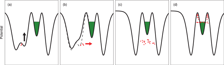
Figure 2. Basic mixing scheme in a nested Penning trap: positrons (green) are held at the centre of the trap and antiprotons (red) are brought in by potential manipulations. (a) Antiprotons held in a small side well before injection. (b) The side well is removed and antiprotons stream through the positrons. (c) Antiprotons bounce to-and-fro through the positrons and cool by the interaction. (d) Antiprotons eventually cool to the level of the positrons, and some become captured in the side wells via field ionization of weakly bound antihydrogen.
Download figure:
Standard image High-resolution imageA detailed analysis of the axial (i.e., along the z-direction) distribution of the antihydrogen annihilations [78] revealed that it could not be accounted for if it was assumed that the antiprotons formed antihydrogen after reaching thermal equilibrium with the assumed temperature of the positron plasma (which was taken as the ambient temperature of the ATHENA trap of 15 K). Indeed the antihydrogen temperature(s) used to fit the distributions were around two orders of magnitude higher than that value. The highly pertinent conclusion from that work was that this simple method of antiproton–positron mixing was unlikely to form antihydrogen with kinetic energies low enough to be held in a sub-kelvin-deep neutral atom trap and that other techniques needed to be developed if the goal of trapping was to be achieved.
As an alternative to producing antihydrogen by launching energetic antiprotons into positrons and waiting for the excess energy to be lost by collisions, one can start with cold antiprotons 'below' the positron space charge, and drive them into the positrons in order to reduce the excess energy involved in the process. Charged particles held in Penning-type traps possess an axial bounce frequency, fz, that is the rate at which the particles traverse and return to their original position in the longitudinal (z) direction in the trap. Applying an oscillating, axially oriented, electric field at this frequency can excite the longitudinal motion of, for example, antiprotons, and give them energy to overcome the potential separating them from the positrons.
In all but ideal Penning traps, the electric potential confining antiprotons is anharmonic: the frequency of the longitudinal motion will depend on the longitudinal energy of the particle, with lower amplitudes tending towards simple harmonic motion. As a consequence, driving the particles at a single frequency does not resonantly excite any individual antiproton into the neighbouring positrons. In order to initiate mixing in this manner, one relies on large driving amplitudes, and/or heating of the particle distribution to achieve injection. This technique was first demonstrated by ATRAP [31]. In that scenario, a 825 kHz drive with a 1 V peak-to-peak amplitude was applied for many seconds, with the frequency chosen to be resonant with the axial bounce frequency for antiprotons oscillating near the axis and near the bottom of their nested potential well. Further discussion of this technique is given in the review by Gabrielse [32], including details of antihydrogen detection and an exploration of using weaker radio frequency drives.
The ALPHA collaboration has solved the problems associated with the distribution-heating resulting from a fixed drive by developing a chirped frequency excitation technique, based upon the phenomenon known as autoresonance, that rapidly excites all antiprotons coherently to the positron energy using low-amplitude excitation (≤50 mV) [79]. This mixing scheme has been used for all ALPHA trapping experiments to date, and is discussed in detail in section 4.4.
In a recent demonstration of antihydrogen trapping [80], ATRAP have used another variant on the driven technique. In order to maintain resonance with the antiprotons as the axial oscillation becomes anharmonic they have applied a driving force with a frequency spectrum broadened by noise for a period of up to 10 min. Other experiments were undertaken, in a manner similar to ALPHA's autoresonant technique, using a chirped drive with the chirp duration varied for periods of between 2 ms and 15 min. No further details were provided.
3. Antihydrogen detection via annihilation and field ionization
3.1. Annihilation
When antihydrogen is formed (in the absence of a neutral atom trap), it is likely to promptly (within a few microseconds) migrate to the electrode wall of the charged particle trap where it will annihilate on contact. The antiproton annihilation with nuclear matter results in the release of pions, several of which (typically two or three) may be charged. These pions are sufficiently energetic that they penetrate the walls of the vacuum chamber and other materials which may surround the trap, and can then be registered using external detectors. Positron–electron annihilation is almost exclusively accompanied by the emission of a pair of back-to-back gamma rays each with an energy close to  = 511 keV, with me the positron/electron rest mass and c the speed of light. Over the years, a number of different technologies have been used to detect the annihilation products associated with antihydrogen (e.g. [30, 75, 81]), but we will discuss the ATHENA detector here in detail, as it provided the first conclusive detection of cold antihydrogen through temporally and spatially coincident detection of the antiproton and positron annihilations.
ATHENA's detection system had the dual capability to register the pions using a double layer silicon-strip detector, and the gamma rays with a ring of 192 CsI scintillation devices, arranged in 16 lines of 12. In ATHENA's original work [29], the production of cold antihydrogen was first identified by isolating events where a clear antiproton annihilation vertex (see below) was accompanied by the pair of gamma rays. An entire event was reconstructed only around 0.25% of the time, principally due to the inefficiency with which the gamma rays were detected. Fortunately, ATHENA were able to quickly establish that the antiproton annihilations alone could be used as a useful proxy for antihydrogen formation [77], such that experimental work could progress without the requirement that the positron annihilation be registered. Sources of background antiproton annihilations on vacuum rest gas, as a result of transport to the electrode wall, or perhaps due to the interaction with positive ions that may be trapped with the positrons, were identified (see e.g., [82, 83]) and largely eliminated in later work. Thus, ALPHA's antihydrogen detector was comprised solely of an antiproton imaging system.
A schematic illustration of the inner section of ALPHA is given in figure 3. The antiproton annihilation point, or vertex, is reconstructed using the three-layer silicon detector shown in the figure. This device has been described in detail elsewhere [53, 84]. In brief, the instrument consists of 60 separate modules arranged symmetrically in two halves, and in three barrel-like layers, around ALPHA's antihydrogen trap. Each module has a double-sided silicon layer, which produces a signal to register the passage of a charged pion, which deposits energy directly into the device. Reading out the positions at which each layer of the detector was struck allows the pion trajectory to be reconstructed, and the annihilation vertex to be pin-pointed. A thorough description of the event reconstruction procedures has been given elsewhere [85]. The final vertex reconstruction resolution is 7–8 mm (due mainly to pion scattering in the material between the annihilation event and the detector: see figure 3) and the overall annihilation reconstruction efficiency is around 60% [85]. An example reconstruction of an antihydrogen annihilation is given in figure 4, along with a cosmic ray event—the latter were the main source of background in the trapping experiments and careful filtering procedures were developed to distinguish between these two types of occurrence (see [53, 85] and the discussion in section 5.1.1).

Figure 3. Schematic of the central part of the ALPHA Apparatus showing the electrodes (yellow) the neutral trap magnets (red and orange) and the annihilation detector (blue). The solenoid providing the main axial Penning trap field is not shown.
Download figure:
Standard image High-resolution image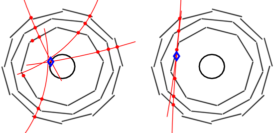
Figure 4. Reconstructed events in the ALPHA annihilation detector. Left: reconstructed vertex of an antiproton annihilation with four tracks. Right: reconstructed background (cosmic) charged particle passing through the detector, which the reconstruction algorithm has interpreted as two almost collinear tracks. The three layers of the detector are shown as the three outer concentric polygon-like layers, and inner surface of the Penning trap electrodes as the inner circular ring. The red points are locations where charged deposits have been identified, red curved lines are fitted helical tracks, and the blue diamond is the location of the reconstructed vertex.
Download figure:
Standard image High-resolution image3.2. Field ionization
The antihydrogen atoms produced via the three-body reaction described in section 2.3 are loosely bound, as has been summarized in various reviews (e.g., [23, 32]), and their behaviour is therefore susceptible to influence from relatively weak ambient fields. These can be both the external electric and magnetic fields of the traps and any self-field from the particles. The latter typically arises from the positron plasma in which the electric fields can be a few 10's Vcm−1. A detailed discussion of some of the phenomena that can occur when antihydrogen is formed in a dense positron plasma has been given by Jonsell and co-workers [86]. The effects of field ionization have been noticed by most antihydrogen collaborations using nested Penning traps. Upon antihydrogen formation, some antiprotons become separated from their parent cloud after forming the neutral, which is then field ionized, leaving them axially and/or radially isolated (see e.g. [65]).
Of interest here is the deliberate field ionization of the loosely bound states, as a means of monitoring the formation of antihydrogen. Field ionization, followed by detection of one or more of the liberated particles, is a standard technique in Rydberg atom physics [87]. Electric fields Fz, here as applied along the z-axis due to the presence of the strong axial magnetic field, will field ionize atoms of radial extent  (with e the unit charge and
  the permittivity of free space)—see [87] for corrections to this simple estimate—with ρ on the order of micrometres, corresponding to binding energies in the milli-electronvolt range.
This technique was pioneered in the antihydrogen field by the ATRAP collaboration [30]. A schematic of their early electrode system, together with the electrical potential on-axis and a representation of the relevant electric fields [30], is shown in figure 5. Antihydrogen travelling along the axis must first pass through an electric field located to the right of the trapped particles in figure 5, where some of the weakest bound states will be stripped. Importantly, this field also prevents antiprotons in the nested trap side well from leaking into the ionization well. The positron may then be stripped in the ionization well (and some information gleaned as to the antihydrogen binding energy [30, 31]), whereupon the remnant antiprotons can be stored, essentially for indefinite periods. Although the technique is inherently inefficient due to the limited solid angle, as the antihydrogen has to travel 3–4 cm to reach the ionization well, there is negligible background on the signal recorded. Antiprotons can be accumulated at will in the ionization well and then ejected in a narrow (∼20 ms) time window to annihilate upon striking an electrode. An example is given in figure 5(c).

Figure 5. Antihydrogen formation and detection by field ionization in the ATRAP experiment: (a) electrodes with a representation of the electric field strength. (b) Potential on axis before and after (full) and during (dashed) injection of antiprotons. (c) Antiprotons from field ionized  released in a 20 ms ejection. (d) Same as (c) but from an experiment without positrons present in the nested trap. Reprinted with permission from [30]. © 2002 American Physical Society.
Download figure:
Standard image High-resolution imageThe field-ionziation technique was also applied by ASACUSA to set an upper bound on the state of antihydrogen detected downstream of the cusp trap on their spectrometer beamline [81].
4. New capabilities
Trapping antihydrogen atoms is a challenging endeavour and several new experimental techniques have been devised to overcome difficulties that have presented themselves along the way. These include refinement of classical magnetic-minimum atom traps, evaporative and adiabatic cooling of plasmas to reach temperatures below those achievable with electron cooling and new mixing techniques to produce lower energy anti-atoms. Additionally, new techniques such as in situ magnetometry using trapped plasmas have been developed to address some of the systematics associated with future spectroscopic measurements.
4.1. Magnetic traps for antihydrogen
Hydrogen (and antihydrogen) atoms possess a small permanent magnetic dipole moment  , which, in the presence of a magnetic field
  , of magnitude B, has an associated potential energy

In free space, Maxwell's equations prohibit a static three-dimensional maximum of magnetic field, though a three-dimensional minimum is realizable, allowing traps for atoms with a component of  antiparallel to
  to be constructed.
The ground state of antihydrogen has a spin of 1/2, and so has only two possible orientations, high-field seeking and low-field seeking, both with a magnetic moment of one Bohr magneton. An additional requirement for stable trapping is that the magnetic field experienced by the atom does not significantly change during the period of the Larmor precession,  , with g here the electron g-factor. This is easily satisfied under realistic experimental conditions.
The condition that an antihydrogen atom is trapped, then, is that the atom's maximum kinetic energy is less than the difference between the minimum value of U from equation (5) and the point with the lowest value of U where the atom can escape the trap (which might be a saddle point or a material surface). The depth of the trap, and the energy of the atoms are conventionally described in units of kelvin, with the Boltzmann constant  as an implied conversion factor to energy units.
A common form of magnetic-minimum trap is the Ioffe–Pritchard configuration, as used by the ALPHA and ATRAP experiments. A novel device, the cusp trap, has been constructed by the ASACUSA experiment. Both forms of traps have the advantage that the magnetic field is purely static, and so strong fields can be produced using superconductors.
4.1.1. Multipole Ioffe–Pritchard traps
The prototypical Ioffe–Pritchard trap consists of a transverse multipole magnet that produces a minimum in magnetic field transverse to the cylindrical axis and two short solenoids (known as 'mirror coils') to produce a magnetic minimum along the axis [88]. These coils are shown in orange and red in figure 3. Near the minimum of the trap, where the magnetic field, and hence the Larmor frequency, is small, Majorana spin flips between high- and low-field seeking states can cause loss of atoms [89]. To counter this, an additional uniform magnetic field is directed along the axis. In antihydrogen experiments, this field is strong (∼T ) as it also serves to transversely confine charged particles in the Penning traps.
A consequence of the non-cylindrically symmetric transverse magnetic field of the multipole is that it can disrupt the aforementioned charged particle confinement. In the most extreme case, particles residing outside a critical radius follow a magnetic field line that crosses an electrode surface over the length of an axial oscillation, and are immediately lost [90]. Even outside this regime, measurements on non-neutral plasmas stored in a quadrupole demonstrated an increased rate of diffusion in the transverse direction, thus reducing the storage time and possibly resulting in heating through the release of electrostatic potential energy [91].
It is desirable, therefore, to minimize the strength of the transverse magnetic field to which the trapped plasmas are exposed. Because the latter are confined in a narrow region near the axis of the trap, this can be achieved by choosing a high-order multipole, since for a multipole of order l, the transverse magnetic field  scales as
  . A large l reduces the magnetic field at small r, but the high gradient near the trap edge means that it is important that the current-carrying windings are as close as possible to the trap boundary, or a large fraction of the trap depth is lost. Figure 6 illustrates both of these aspects, where it has been assumed that the maximum sustainable magnetic field near the coil windings (situated at RMag) is the same for each multipole order.
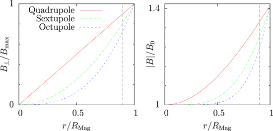
Figure 6. Figure showing the relative B-field strength for several transverse multi-pole magnets. Left: the radial field from a multipole as a function of radius. Right: relative total magnetic field strength of a transverse multipole superposed on a solenoidal field of the same strength as the multipole at the wall ( ). The vertical dashed line in each plot indicates the radius associated with the inner diameter of the ALPHA Penning trap electrodes.
Download figure:
Standard image High-resolution imageALPHA constructed an octupole (l = 4) based magnetic trap with a transverse magnetic field of 1.54 T at the inner radius of the trap (rw = 22.275 mm). The mirror coils, located 137 mm to either side of the trap centre, produced a magnetic field of 1.0 T near their centres [92]. These fields combined with a solenoidal field of 1.0 T to give a trap depth of 0.8 T, equivalent to an energy of 0.54 K kB for ground state antihydrogen. The trap depth was maximized by winding the superconducting wire directly onto the outer wall of the vacuum chamber and using electrodes with a wall thickness of less than 1 mm. Measurements of the temperature of plasmas in the octupolar field showed significant heating rates, which could be reduced by using plasmas with smaller radii [93], which was taken as a validation of the choice of the higher-order magnetic field.
ATRAP initially constructed a magnetic trap using a quadrupolar (l = 2) transverse field, with a depth of 0.56 T, corresponding to 0.38 K kB, and a volume of radius 18.0 mm and length 220 mm [94]. In 2011–2014, they constructed a new generation of their experiment that allows either a quadrupolar or octupolar configuration to be selected [95].
In 2012, ALPHA constructed a second generation trap following the same geometry as the previous device, but including a total of five short solenoids spaced along the trapping region. The additional coils are intended to be used to vary the length of the magnetic trap and to cancel field inhomogeneities [96].
Both ALPHA and ATRAP have reported trapping antihydrogen [80, 97]. Key to both demonstrations was the need to de-energize the traps to allow the antihydrogen atoms to escape, annihilate and be detected. The annihilation detectors used are also sensitive to cosmic rays, which forms a background. Minimizing the length of time over which the atoms escape proportionately reduces the number of background counts, and a significant improvement in signal-to-noise can be obtained. ALPHA implemented a rapid-shutdown system, in which the current from the magnets was switched through a dissipative resistor network using a high speed insulated-gate bipolar transistor device. Coupled with a low inductance design for the magnets, this allowed the magnetic fields to be shut off with a decay constant of 8 ms for the mirror coils and 9 ms for the octupole. They defined a 30 ms annihilation detection window in which the trap depth had decayed to less than 1% of its original value [92].
ATRAP's original magnet, not originally designed for rapid shutdown, could be ramped off in around 1 min. However, by purposefully inducing a quench in the superconductor by heating the coils, this could be improved to around 1 s, albeit with a long recovery time required afterwards. Recently, ATRAP have constructed a new magnet, which is designed to be operated as either a quadrupole or octupole, and can be turned off in tens of milliseconds.
4.1.2. Cusp trap
An alternative to the Ioffe–Pritchard trap is a system of coils in the anti-Helmholtz configuration. These produce a cylindrically symmetric magnetic field, but with a zero at the minimum. Atoms will be lost via Majorana transitions here, and consequently the trapped lifetime will be reduced. In this scheme, depicted in figure 7, antihydrogen is produced in a region of stronger magnetic field, displaced along the cylindrical axis from the minimum. Low field seeking atoms tend to be focused and extracted along the axis, while high field seeking atoms are defocussed. This produces a spin-polarized beam of antihydrogen directed along the axis of cylindrical symmetry that can be used for ground-state hyperfine spectroscopy, by passing the beam through a radio-frequency cavity to induce resonant transitions between the spin states, coupled with spin-state-selective detection. An interaction and detection region placed along the axis can interact with the atoms while being outside a region of strongly inhomogeneous magnetic field, in principle allowing for high-precision spectroscopy [98]. An additional advantage of this scheme is that significant focusing and polarization of the atoms can be achieved at temperatures much higher than those needed to stably trap the atoms. ASACUSA's cusp trap is expected to produce a polarization as high as 99% at temperatures up to 5 K [99].

Figure 7. Schematic of the cusp trap scheme (reprinted with permission from [100]). (a) Cross sectional view of cusp trap with  detector. The magnetic field lines are superimposed. (b) Electric potential configuration along the axis, showing the nested trap for
  formation and the field ionization trap (FIT) for
  detection.
Download figure:
Standard image High-resolution image4.2. Evaporative cooling
4.2.1. Background
In the Penning traps used by the antihydrogen experiments, it was thought that the non-neutral plasmas would radiatively cool to the cryogenic temperature of the surrounding apparatus (∼8 K). In ALPHA however, direct measurements, using the technique of [101] showed equilibrium values well above this. The mechanisms through which the temperature is elevated are not known, but hypotheses include electronic noise coupled to the electrode potentials, black-body radiation from far-away, but warmer, parts of the apparatus, or transverse expansion due to slight misalignments of the magnetic field accompanied by conversion of electrostatic energy to thermal motion. This last option is further exacerbated in the inhomogeneous Ioffe trap fields, where enhanced diffusion is expected [102], and has been observed to lead to higher temperatures.
Evaporative cooling was first demonstrated by Kleppner and co-workers for a trapped gas of hydrogen [103], later extended to alkali atoms, and is nowadays widely used to cool ensembles of trapped atoms [104]. It is the most widely used route to achieving Bose–Einstein condensates of dilute gases, a field that has attracted intense study in recent years. While widely used for neutral atomic species, evaporative cooling on charged particles at cryogenic temperatures had not been demonstrated before 2010, when ALPHA cooled antiproton clouds to temperatures as low as  K.
K.
Evaporative cooling requires two basic mechanisms to be effective. First, it must be possible to selectively remove high-energy particles from the distribution. This can be approached in a number of ways, including controlling the depth of the trapping well, or by inducing an atomic transition in the highest-energy species. Secondly, the ensemble should thermalize on a timescale comparable to, or shorter than, the time over which evaporation takes place. This process is typically driven by elastic collisions in the ensemble.
Evaporative cooling operates by truncating a thermal distribution above some high energy cut-off. Atoms that, through collisions, have an energy higher than this cut-off are ejected from the trap. The loss of these high-energy particles results in a net reduction of total energy of the remaining distribution. The distribution then re-thermalizes through collisions and achieves a lower temperature. As the temperature of the distribution falls, the number of particles able to escape becomes negligible, so then the truncation energy must be reduced if further cooling is desired. Additionally, as antiprotons are lost, the space charge of the cloud falls, which also increases the confinement barrier. However, the size of this effect is small, on the order of 1 μeV per antiproton lost. Cooling can continue in this fashion, in principle, until there are no particles remaining.
The process can be described using two coupled rate equations

and

where N is the number of atoms in the ensemble at a temperature, T,  describes the timescale of the evaporation, and α is the ratio of the average energy removed by an evaporating particle compared to the average energy of a trapped particle [105].
The evaporation timescale,  is the rate at which particles are scattered into the unconfined portion of the thermal distribution. It is determined by the timescale over which energy is resdistributed through collisions,
  , and the truncated fraction of the well, parametrized by
  , the ratio of the well depth to the temperature. A detailed analysis [105] leads to the relationship (valid for
  )
)

for evaporation along one-dimension only, which is the most appropriate for evaporative cooling in a Penning trap. This is a factor of  higher than the equivalent expression for evaporating atoms [104], reflecting the lower evaporation rate for charged particles.
The exponential dependence on η in equation (8) means that the evaporation rate drops dramatically for large η. This effect is so marked that η tends to a constant value for a wide range of parameters in a given experiment, and T is a function of UW only. In evaporative cooling with antiprotons, ALPHA found values of η of order 12.
4.2.2. Measurements
ALPHA's implementation of evaporative cooling on antiprotons began with a cloud of ∼45 000 antiprotons of radius 0.6 mm and density  , at a temperature of 1000 K. The well depth was reduced by manipulating the electrode voltages, from an initial value of 1.5 V to final values as low as 10 mV. Temperature measurements at several different well depths are shown in figure 8. The increasing slope, inversely proportional to temperature, shows cooling with reducing well depth, and the falling number of particles is also visible [106]. The phase-space density of the low-energy particles increases, indicating true cooling, rather than simple truncation of the original distribution.

Figure 8. Evaporative cooling of antiprotons. Integrated antiproton loss as a function of well depth for experiments that evaporatively cooled the antiprotons by lowering the well to different depths. The shallower the well, the lower the temperature of the remaining particles. Reprinted from [106]. Copyright 2010 by the American Physical Society.
Download figure:
Standard image High-resolution imageFrom the initial distribution, ALPHA produced cold antiproton clouds with a temperature of (9 ± 4) K, with ( of the particles remaining. This increased the number of particles with energies less than the trap depth (0.5 K) from less than one to on the order of ten. Also, the observed scaling of the number of particles lost and the temperature of the remainder followed the form predicted by the simple model encapsulated by equations (6) and (7) closely, thereby validating the underlying assumptions. A later application of evaporative cooling to positrons and electrons, which can be produced in plasmas of much higher density, showed behaviour that was qualitatively similar, but on shorter timescales, as might be expected from the higher collision and cyclotron radiation rates.
Evaporative cooling was instrumental in the successful trapping of antihydrogen atoms [97], as it reduced, for the first time, both the positron and antiproton temperatures to the range (below 100 K or so) where non-negligible numbers of antihydrogen atoms could be expected to have trappable energies.
4.2.3. Limits
Evaporative cooling is subject to both technical and physics limits. The technical—loss of the charged particles through annihilation or other loss processes, and noise on the voltages applied to the Penning trap electrodes can, in principle at least, be alleviated with higher quality vacuum and magnetic fields, and with quieter and more finely adjustable electronics. The physical limitations stem from the difficulty in maintaining a high collision rate as particles are lost and the ensemble cools, and there are two principal processes that contribute to this.
The height of the barrier confining the plasma is at a minimum on-axis, and this is where most of the particles escape. The resulting hollow density distribution is unstable and is quickly filled-in by charge from higher radii. These particles lose angular momentum, and to conserve total angular momentum, charge also migrates outwards, causing the plasma to expand and, as a consequence, the density and collision rate to fall. There is an additional heating term associated with this process, from the conversion of electrostatic potential energy to kinetic energy of the particles. This has been calculated to be small, however, equivalent to a 5 mK rise in temperature for each antiproton lost.
The rate at which a plasma equilibrates through collisions is a strong function of the degree of magnetization, which is parameterized by  , where
  is twice the classical distance of closest approach and
  is the radius of the cyclotron orbit [107]. κ scales with the plasma temperature as
  . For
. For  (i.e., in the highly magnetized regime) the collisional equipartition rate scales as
  —the rate is exponentially suppressed at low temperatures. For antiprotons in a 1 T magnetic field (as in ALPHA),
  corresponds to a temperature of 8.5 K. To achieve temperatures much lower than this, experiments will need to operate at lower magnetic fields, as well as preparing as high an initial density of particles as possible.
4.3. Adiabatic cooling
Adiabatic cooling relies on the existence of the quantity invariant under the assumption of adiabaticity

where the integral is taken over the turning points of the motion (at a and b), and  is the component of the velocity parallel to the magnetic field. In a one-dimensional harmonic potential
  , this can be expressed more simply as

where E is the particle's energy. Reducing  in an adiabatic manner results in a corresponding reduction in E, which, averaged over a distribution of energies, is equivalent to cooling. Energy remains conserved as the potential does negative work to increase the distribution's volume and decrease its temperature, without a change in entropy. The adiabatic condition is fulfilled if the oscillation frequency changes very little over one oscillation period, i.e.

The technique was demonstrated by ATRAP, using between  and
and  antiprotons in a 3.7 T magnetic field [108]. The antiproton plasmas were placed in a harmonic well with an initial oscillation frequency
  between
  and
and  , and then the frequency lowered until the particles escaped the well. The final frequency
  was taken to be that given by the well just before the plasma escaped, and was found to be constant for all of the measurements.
The temperatures for different degrees of expansion are shown in figure 9 and follow a power law  until approximately
  × 500 kHz, where the temperature levels out. The lowest temperatures are
  0.7) K, for plasmas expanded by more than a factor of 10. Later work [109] explained the limit in temperature as being due to imperfect equilibration for the higher values of
  , and achieved a good reproduction of the experimental results using a numerical model.

Figure 9. Measured and predicted temperatures, T, for 5 × 10⁵ antiprotons after adiabatic cooling. The measured T fits a power law (solid curve) down to the lowest measured value (grey band) (reprinted with permission from [108]. © American Physical Society). Note that fi here is equal to  in the text.
Download figure:
Standard image High-resolution imageAntiprotons cooled using this method have not yet been reported to have been used to produce antihydrogen. Note that because the length of the antiproton cloud increases during adiabatic cooling, this process conserves phase-space. The large increase in the antiproton volume is, however, likely to pose difficulties in the inhomogeneous magnetic trapping fields.
4.4. Mixing via autoresonant injection
As described elsewhere herein, the most widely used technique to produce antihydrogen atoms from antiproton–positron combination is to confine the constituent particles in an overlapping volume, and allow them to interact. To achieve this, a 'nested-well' potential is used (as depicted in figures 2 and 7), typically with the positrons occupying the central well and close to thermal equilibrium, and the antiprotons in an energetically excited state in the outer well.
The typical size of the energy barrier that the antiprotons need to overcome to enter the positron plasma must be at least several times the positron plasma temperature. Some of the lowest temperatures measured under antihydrogen trapping conditions have been on the order of 40 K, which necessitates a barrier of around 200–400 K, or a few tens of milli-electronvolts.
A complication arises from the dependence of the barrier height on the space charge of both constituent species, though primarily the positrons, due to their higher density. Unavoidable fluctuations (on a shot-to-shot basis) in the number of particles prepared for mixing result in corresponding changes in the space charge level. Experimentally, such variations are usually around 10%, and given that the positron space charge is of order 1 eV, this results in deviations of around 100 meV, which are large compared to the depth of the neutral atom trap (50 μeV).
In the early phase of antihydrogen physics, the energy of the anti-atom was not a critical parameter, and the antiprotons were released into the positrons well above their space charge level. Initially, it was thought that the antiprotons would come into thermal equilibrium with the positrons before forming antihydrogen, such that the anti-atom would possess a temperature close to that of the positrons, regardless of the antiproton energy distribution. Later experiments [78] showed that this was not the case, and so a technique that could inject the antiprotons with low kinetic energy was needed.
In the nested potential, the antiprotons reside in an anharmonic potential such that their axial motion can be considered as that of a nonlinear oscillator. There is a well-known and general phenomenon, known as autoresonance, in which the response of a single nonlinear oscillator can become phase-locked to an external swept frequency drive (see e.g., [110]). When this happens, the oscillator matches its frequency and hence its amplitude to the drive. In this way, the amplitude of oscillations can be precisely controlled. It was demonstrated by ALPHA [79] that the bulk oscillation of an antiproton plasma could be controlled in this manner. Barth and co-workers have also presented a theoretical treatment of the process [111].
Figure 10 shows a typical set of potentials used in ALPHA for autoresonant injection of antiprotons into positrons, and the axial bounce frequency-energy relationship for the former. It is apparent that the positron plasma alters the vacuum potential to a large extent, so the total potential is calculated numerically by self-consistently solving the Poisson and Boltzmann equations, knowing the confining potential, the radial distribution of the positrons and their temperature [54]. At the energy at which the antiprotons should pass into the positrons, the oscillation frequency becomes zero, which is impossible to realize. One would presume therefore, that it is not possible to achieve injection in this way. However, experimentally, we observe that sweeping the drive frequency close enough to this level injects a large fraction of the antiprotons. The optimum final frequency is determined experimentally, and is on the order of 250 kHz for the potentials typical of ALPHA. Importantly, the final drive frequency corresponds to a fixed difference in energy between the space charge level of the positrons and the nominal oscillator amplitude. Therefore, the injection technique is robust against fluctuations in the positron space-charge level.

Figure 10. Autoresonant mixing: left: depiction of a typical on-axis nested Penning trap potential with (red) and without (blue-dashed) positrons in the central well, with the former accounting for their space charge. Right: calculation of the oscillation frequency of an antiproton as a function of its energy in the left side-well of the nested potential. The energy is given relative to the central potential in the presence of positrons such that the energy is zero when the antiprotons just pass though the positrons (and the frequency therefore goes to zero).
Download figure:
Standard image High-resolution imageA second advantage of autoresonance is that since the antiprotons are injected with minimal kinetic energy, antihydrogen formation begins quickly. A long wait to allow the species to match velocities and begin recombination would allow collisions amongst the antiprotons to redistribute energy from the axial motion to the transverse degrees of freedom, which would result in hotter, untrappable antihydrogen.
4.5. Magnetometry
Precise measurements of atomic transition frequencies in a magnetic trap require detailed knowledge of the trap's magnetic field, since the energy levels of the atom are shifted by the magnetic field. For measurements of the ground-state hyperfine intervals, this is of vital importance, since the energy difference between the trapped and untrapped manifolds is, to a good approximation, directly proportional in the magnetic field. The 1S–2S transition frequency is also shifted by a magnetic field, by an amount  HzT−1 [112].
Technical considerations, not least space constraints, make an in situ measurement of the magnetic field using conventional sensors difficult to achieve. A more fruitful approach is to use atoms or particles with easily measurable and well-known magnetic field dependent properties to determine the magnetic field.
For ALPHA's measurement of the ground-state hyperfine transition, [113], injected microwaves were used to excite the cyclotron frequency of electrons trapped in a spheroidal plasma at various locations on the trap axis, while the energy transfer was monitored by non-destructively measuring the shift in the plasma temperature [114]. By varying the frequency of the microwaves, the electron-cyclotron resonance (ECR) of the plasma could be mapped out, from which the magnetic field in the plasma could be determined. This technique achieved a precision of 3.6 parts in 105, with a possible systematic shift of around 1 part in 103. In the ALPHA apparatus, the technique was limited by the geometry of the trapped plasma, and the unknown mode structure of the microwaves used to excite the cyclotron resonance. Ultimately such a technique will be limited by broadening from Coulomb scattering to approximately 1 part in 106. However, the technique benefits from being straightforward to employ in many locations throughout the trap, a feat which would otherwise not be possible with other sorts of ECR measurements that typically require a specific electrode set with a highly tuned tank circuit for detection.
For higher-precision measurements of the magnetic field it will be necessary to use a different trapped species, such as a trapped ion or atom with an accessible, magnetic-field sensitive transition in the optical regime. This will also avoid the effects associated with the frequency-dependent microwave mode structure typical of a practical antihydrogen trapping experiment.
5. Trapping and beaming antihydrogen
Currently, it is thought that measurements on antihydrogen will be carried out with two broad categories of cold antihydrogen. (i) Trapped antihydrogen atoms that are confined in some spatial volume by magnetic fields and are necessarily cold (<1 K) owing to the available trap depths; and (ii) beamed antihydrogen, which involves directing a population of the anti-atom in a known state, and conducting in-flight measurements upon them. We will describe the first topic in depth, as it represents by far the largest category of antihydrogen atoms available for measurement at the time of writing, and follow with a brief discussion of the second topic.
5.1. Identifying trapped antihydrogen
Because of the difficulty inherent in producing large samples of low-energy antihydrogen atoms, only a few have been trapped relative to the number produced in experiments to date. (In ALPHA, for example, this is approximately 1 in 10 000 antihydrogen atoms produced.) Consequently, verifying that antihydrogen was actually being trapped was an initial challenge, and (still) depends on extracting a small signal from a much larger background. A crude way to test for antihydrogen trapping is to empty the trap (for example, by de-energizing its magnetic fields), and search for the resulting antiproton annihilation signal using a detector. In this scheme, the two main backgrounds are detector signals from cosmic-ray particles that mimic antiproton annihilations, and annihilations from antiprotons trapped in the magnetic trap as singular charged particles rather than as part of an antihydrogen atom. We will discuss these topics in some depth with respect to the ALPHA experiment, but other experiments have similar issues, though dependent on the trap and detector technology used.
5.1.1. Cosmic-ray background
ALPHA utilizes a silicon vertex tracking detector to identify antiproton annihilation events. Cosmic rays striking the Earth's atmosphere produce showers of charged particles, some of which (mainly muons) reach ground level. Muons passing through the silicon detector leave charge deposits and trigger the logic that reads out the position information from the silicon modules. The reconstruction and analysis procedure classifies sets of three hits in three layers of the detector as a single track, and extrapolates two or more such tracks to identify an annihilation vertex. The stereotypical cosmic ray event (such as that shown in figure 4) leaves deposits in a more-or-less straight line, and can be discarded. Often however, the charged particle can be deflected in the magnetic field, so that the hits do not lie along a straight line, or the particle may disintegrate, producing several tracks from daughter species. Such events can be mis-identified as antiproton annihilations, and therefore constitute an important background.
To distinguish cosmic-ray events from annihilations, a set of detector data criteria ('cuts') was developed to maximize both rejection of cosmic rays and acceptance of annihilations. These criteria were made up of limits on the maximum squared residual from the best straight line fit to the hits making up the tracks contributing to the vertex, and the maximum distance from the centre of the trap. In ALPHA's work, to be accepted as an antiproton annihilation, a reconstructed vertex was required to be within 4 cm of the trap axis. In addition, when an event had three or more tracks, the squared residual from the best-fit straight line was required to be greater than 0.05 cm2, and otherwise greater than 2 cm2. These criteria were optimized by maximizing the statistical significance of a given number of signal events, scaled by the acceptance measured using an almost-pure sample of annihilations recorded during mixing, against a measured background on a pure cosmic-ray data set. The completed criteria reduced the cosmic-ray background to a rate of 0.022 s−1, while retaining ∼42% of antiproton annihilations.
In ALPHA, the time measurement window for detecting antihydrogen atoms released from a rapid shutdown of the atom trap magnets is 30 ms, which leads to the mis-identification of a cosmic ray as an annihilation once in about 1500 trials on average.
5.1.2. Mirror-trapped antiprotons
With the level of rejection described above, cosmic rays do not pose a significant background in the magnet shutdown time window. However, interpreting annihilation events that occur in that window is problematic if there are some means by which antiprotons can be present in the trap in addition to antihydrogen atoms, since the detector is unable to distinguish these two events. A possible source of this background is so-called mirror-trapped antiprotons.
The magnetic-minimum used to trap antihydrogen atoms can also confine charged particles. The trapping mechanism arises from the adiabatic invariance of the magnetic moment,  , of a charged particle orbit, given by:

where  is the component of velocity perpendicular to the magnetic field of magnitude B, and
  the associated kinetic energy. As the particle moves from low to high magnetic field, energy is transferred from the parallel to perpendicular degrees of freedom. The particle will be reflected from the region of high magnetic field if the perpendicular energy is sufficiently high such that

where  and
and  are the maximum and minimum of magnetic fields for particles with energy
  and
and  (kinetic energy in the motions perpendicular to and parallel to the magnetic field) at the field minimum. The end-coils of the Ioffe trap form a 'mirror-trap' for antiprotons with at least this division of parallel and perpendicular energy, and any that are held in this manner would be released from the trap when it was shut off.
Electric fields can be used to overcome the mirror trapping force and remove the antiprotons from the trap, but such an approach is not perfect, as one can always imagine ever larger ratios of perpendicular to parallel energy in the particle which would remain trapped. The motion of antiprotons in the actual electric and magnetic fields used in the experiments is not simple, and is best analysed via numerical simulations. In ALPHA, these indicated that only antiprotons with  greater than 20 eV would remain trapped when the highest easily achievable electric field, around 200 Vm−1, was used. Additionally, the simulations revealed that trapped antiprotons would be deflected by an electric field as they escape. Figure 11 shows the expected distributions of time (t) and axial coordinate (z) of the annihilation for both antihydrogen atoms and mirror-trapped antiprotons subject to different electric field configurations. Comparison of the observed distributions of these variables with the simulations allows mirror-trapped antiprotons to be distinguished from trapped antihydrogen atoms. Reference [115] discusses the topic in depth in the context of the ALPHA experiment.

Figure 11. Axial annihilation positions versus time after de-energizing the ALPHA magnets. The magnetic field decays to effectively zero in 30 ms. Top: simulation of antihydrogen (grey dots) overlayed with the experimental data. Bottom: simulation of antiprotons with  20 eV (small coloured dots) overlayed with the measured events. The colours indicate the type of experiment as indicated in the legend [97], with electric fields biased either to left or right along z.
Download figure:
Standard image High-resolution image5.1.3. Trapped antihydrogen: first events
In 2010, ALPHA reported observation of 38 annihilation-like events in a data set when a contribution of 0.46 ± 0.01 events would be expected from cosmic rays. The data were recorded with three different electric field configurations, and are plotted as the large points in figure 11. The data are clearly incompatible with the mirror-trapped antiproton simulations, but match well with the calculations of the antihydrogen distribution. On the strength of these observations, ALPHA reported the first trapping of antihydrogen atoms [97].
These atoms were held for only ∼172 ms, as their lifetime in the trap was not known. Later experiments stored the anti-atoms for longer times (as shown in figure 12), with some trapped unambiguously for at least 1000 s [116]. This lifetime is consistent with estimates from collisional energy transfer with residual gas atoms. The antihydrogen atoms, as discussed in section 2.3, are typically formed in highly excited states, but decay to the ground state with greater than 99% probability after less than 1 s [116]. The fact that this time is so much shorter than the trap lifetime demonstrates the feasibility of conducting experiments on ground-state antihydrogen atoms.
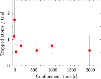
Figure 12. Number of antihydrogen atoms trapped in ALPHA as a function of the holding time after formation [116].
Download figure:
Standard image High-resolution imageIn [97], 38 atoms were observed in 436 trials, or a average of 0.09 per experiment. With further optimization of the experimental parameters, including the positron temperature and density and the autoresonant injection sweep parameters, this was increased to as high as one atom per trial on average, with a cycle time of around 20 min. Even though this is still an extremely small number of atoms compared to typical atomic physics experiments, the easily detectable annihilation signature and the long confinement time can compensate to some extent for the difficulty this introduces.
With larger numbers of trapped antihydrogen atoms, it was also found that their energy distribution matched that of a 50 K Maxwell–Boltzmann distribution, truncated to the 550 mK trap depth [116], consistent with anti-atoms being formed at thermal equilibrium between the positrons and the antiprotons.
In 2012, ATRAP reported detecting 35 annihilations, corresponding to 105 ± 21 trapped antihydrogen atoms, in a total of twenty experiments in which the holding time was varied between 15 and 1000 s, followed by a 1 s magnet quench [80, 117]. ATRAP distinguished the resulting annihilation events from cosmic rays using a combination of a cylinder of scintillating fibres and scintillator paddles arranged around their trap. Coincidence requirements between these detectors, together with the adoption of various event classification criteria [117], reduced the background cosmic flux from 41 to 1.7 s−1, while lowering the annihilation detection efficiency by around 40% to an overall efficiency of 33%. This system could not, however, be used to distinguish the possible release of mirror-trapped antiprotons in the manner described above for the ALPHA detector. Instead, ATRAP argued that there was no plausible mechanism whereby antiprotons with a large excess of transverse energy (more than 137 eV would have been required) could be trapped in their experiment [118] to rule out the possibility that the events observed could have resulted from the release of mirror-trapped antiprotons.
ATRAP used a variety of antiproton–positron mixing procedures to produce the antihydrogen, and details can be found elsewhere [117]. It is notable, though, that their results fluctuated, even for nominally identical trials, due to an inability to achieve sufficient control of the antiparticle clouds during the mixing [80, 117]. Only two of the twenty trials, which each took around two hours to complete, contained evidence for the release of trapped antihydrogen at, or greater than, the  level: one experiment, however, observed the release of 39 ± 8 anti-atoms. The average of the number of simultaneously trapped anti-atoms was found to be 5 ± 1, or 3.5 ± 0.7 if the data were analysed without inclusion of the result from the best trial. Twenty control trials were also performed with the Ioffe trap quench procedure, but without antihydrogen in the trap, and in which no false annihilation signals were recorded.
5.2. Beaming antihydrogen
The ASACUSA and AEgIS experiments both aim to produce a beam of antihydrogen atoms, the former to perform hyperfine spectroscopy in a region free of magnetic field, and the latter to measure the vertical displacement of the beam as it propagates under the influence of gravity. These schemes benefit from removing the complicating effect of the large, inhomogeneous magnetic fields present in the trapping experiments, however at the cost of introducing other complications as discussed below.
5.2.1. ASACUSA
The ASACUSA collaboration aims to perform hyperfine spectroscopy of the ground state of antihydrogen by passing a beam of spin polarized anti-atoms through a low magnetic field region with a microwave cavity intended to resonantly drive hyperfine transitions and then through a sextupole magnet that will separate the two positron spin states on their detector [119] (see e.g. figure 7).
Successful formation of antihydrogen in their trap [75] was reported in 2011, and this was followed in 2014 by the detection of around 100 atoms that had travelled 2.7 m along their spectroscopy apparatus [81]. A significant question remains as to what fraction of the atoms, which are produced in highly excited states, will reach the state-selection region and be in the ground state when they do so. Recent work by ASACUSA has demonstrated that a significant fraction are more tightly bound than n = 29 [81]. This matter has also been addressed using Monte Carlo simulations in an effort to optimize low-n yields for various positron plasma parameters [120].
5.2.2. AEgIS
The AEgIS collaboration plans to make an antihydrogen beam by Stark acceleration of Rydberg anti-atoms. The highly excited antihydrogen is to be made by colliding Rydberg Ps with a cloud of cold antiprotons, similar to the technique discussed in section 2.3. In AEgIS, the excited Ps will, however, be supplied by first implanting positrons in a low-temperature, porous,  target located near a cold antiproton plasma and then resonantly exciting the emerging thermalized ground state Ps to a high n state, in a manner recently demonstrated by Cassidy and coworkers [121]. The Ps atoms will then travel a short distance to the antiproton storage region and form antihydrogen through the charge-exchange reaction, as given by equation (4).
Because the Ps atoms have been laser-excited to a well-defined Rydberg state, the antihydrogen atoms will also be formed in a Rydberg state with a large polarizability. This will allow the atoms to be accelerated horizontally, using an inhomogeneous electric field, to a velocity of several hundred metres per second, a technique which has been demonstrated with Rydberg hydrogen in zero magnetic field [122]. The atoms will then travel along a beamline housing a moiré interferometer in order to probe the influence of gravity [123]. In principle, such a beam can also be re-purposed for spectroscopic measurements. The experiment is currently undergoing commissioning at the CERN AD [124].
5.2.3. GBAR
The GBAR collaboration plans to create a beam of  ions by aiming an antiproton beam at a dense cloud of laser-excited Ps created by implantation of positrons on the inside of a tube made of appropriate porous material. The positron requirements for achieving the required Ps density are beyond that possible with the radioactive source scheme used by all others (see section 2.2), so an electron linac-based accumulation scheme is being pursued [28]. Formation of the
  ion occurs with low overall probability, and it is estimated that only around three ions will be formed per antiproton pulse from ELENA [125].
Once formed, the  ions are to be guided into a radio-frequency trap (a linear Paul trap), where they will be merged with a cloud of laser-cooled Be+ ions and sympathetically cooled to the milli-Kelvin level [126]. A final stage of sympathetic cooling will cool a single
  –Be+ ion-pair to the motional ground state, whereupon a pulsed laser will photo-ionize the
  and the neutral antihydrogen atom will be left to free-fall inside a vertical vacuum chamber. The gravitational acceleration will be calculated by measuring the time between the photo-ionization pulse and the time of the atom's annihilation on the bottom of the apparatus. This idea follows a proposal by Walz and Hänsch [127]. Similarly, these atoms could also be used for spectroscopy measurements. The experiment is currently at the planning and off-site construction stages [126, 128, 129].
6. First experiments on antihydrogen
6.1. Measurement of internal structure
The first experiment manipulating antihydrogen's internal structure was performed by inducing microwave transitions between trapped and untrapped states of the ground state hyperfine manifold (as reported in [113]). The Breit–Rabi diagram for ground state antihydrogen is shown in figure 13. The potential energy of atoms in state  or
or  increases with magnetic field amplitude. Consequently these atoms are attracted to minima of the magnetic field and can be trapped. Conversely, the
  and
and  states are attracted to strong magnetic fields and are untrapped. The transitions
  and
and  correspond to a flip of the positron spin. The transition frequencies are approximately linear in the magnetic field, and are separated by the hyperfine splitting of 1.420 GHz. At the ∼1 T magnetic field used in ALPHA, the
  and
and  transitions occur at approximately 29.7 GHz and 28.3 GHz respectively.
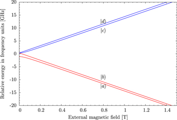
Figure 13. Breit–Rabi diagram of the level-splitting of the antihydrogen 1S ground state as a function of magnetic field. The blue states have anti-parallel (to the B-field) lepton spin and are so-called low-field-seekers (trappable in a B-field minimum), whereas the red states are untrappable. The splitting between the two blue (red) states is due to the antiproton spin.
Download figure:
Standard image High-resolution imageFigure 14 shows calculations of the lineshapes for antihydrogen held in the ALPHA trap. The sharp cut-off at low frequencies corresponds to the trap minimum, while the long tail to high frequencies reflects the fact that the atoms explore most of the inhomogeneous trapping field. In ALPHA's experiment, the trapping volume was illuminated with microwave radiation, swept across a 15 MHz band around each peak [113].

Figure 14. Calculated antihydrogen transition rates fad and fbc for ground state transitions  and
and  respectively for antihydrogen trapped in ALPHA. The long tails to higher frequencies arise as the antihydrogen moves around in the magnetic trap and is exposed to varying magnetic fields.
Download figure:
Standard image High-resolution imageBecause the production process does not significantly bias the formation of particular hyperfine states, the microwave frequency was swapped back-and-forth between fad and fbc, (to drive transitions  and
and  respectively) to ensure that both the trapped
  and
and  populations were addressed during each experimental trial. Because of limited microwave power, the illumination windows were long, with six sweeps of 15 s each for both transitions (180 s total).
Atoms successfully spin-flipped were ejected from the trap and this could be detected in two ways: 'appearance' and 'disappearance'. For the 'appearance' signal, annihilations measured by the annihilation detector during the illumination period were counted. Due to the long interrogation window, this method had a significant cosmic background that was reduced to  s−1 using optimized selection criteria (discussed in detail in [113]). In the 'disappearance' signal, the number of annihilations during the fast shutdown of the magnetic trap after completing the microwave sweeps was counted. In this case, a reduction of the trapping rate indicated that atoms were driven to untrapped states. This procedure constitutes a typical 'on resonance' measurement. The results from this experiment were compared against an 'off resonance' experiment, in which the magnetic field was increased by 3.5 mT, thereby detuning the transition by 100 MHz, but otherwise leaving the experimental procedure unchanged. A further experiment conducted without injecting microwave power but with identical timing ('no microwaves' condition), was used to control for heating of the trap structure by the microwaves that could lead to gas desorption, a poorer vacuum, and consequently a reduced trapped lifetime (creating spurious counts in the 'appearance' measurements or a loss of counts in the 'disappearance' signal).
The disappearance mode measurements are summarized in table 1, and the appearance mode data are shown in figure 15. The significant reduction in the number of trapped atoms seen in disappearance mode and the large peak measured in appearance mode when the microwave radiation is on-resonance when compared to off-resonance demonstrate that the microwave radiation ejected the atoms from the trap. It can be noticed that the number of counts in the off-resonant experiments is smaller than the no-microwaves case in table 1, and that a small peak can be seen in the second 15 s sweep in figure 15. This is likely due to a combination of the the microwave-induced heating of the electrodes and the consequent loss of antihydrogen atoms through interaction with the desorbed material, and the fact that the off-resonant sweep for the  transition has a finite probability to induce
  transitions.
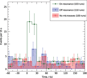
Figure 15. Appearance mode data showing the number of reconstructed annihilation events as a function of time during experiments where the anti-atoms were exposed to either resonant microwaves (green), non-resonant microwaves (blue) or no microwaves (red). Microwave injection was initiated at 0 s, and a pattern of 15 s at fbc followed by 15 s at fad was repeated six times.
Download figure:
Standard image High-resolution imageTable 1. Disappearance mode data showing the number of trapped atoms at the end of trap and hold experiments with different magnetic field and microwave frequency settings.
| Relative | Relative | Number | Number of | Rate | Comment | |
| microwave | magnetic | of |
 atoms atoms |
|||
| frequency | field | trials | remaining | |||
| 1 | 0 MHz | 0 mT | 79 | 1 | 0.01 | On- |
| ± 0.01 | resonance | |||||
| 2 | 0 MHz | +3.5 mT | 88 | 16 | 0.18 | Off- |
| ± 0.05 | resonance | |||||
| 3 | +100 MHz | +3.5 mT | 24 | 1 | 0.04 | On- |
| ± 0.04 | resonance | |||||
| 4 | 0 MHz | +3.5 mT | 22 | 7 | 0.32 | Off- |
| ± 0.12 | resonance | |||||
| 5 | Off | 0 mT | 52 | 17 | 0.33 | No |
| ± 0.08 | microwaves | |||||
| 6 | Off | +3.5 mT | 48 | 23 | 0.48 | No |
| ± 0.10 | microwaves |
This measurement probed the hyperfine transition to a precision of 100 MHz, or a relative precision of  . Higher precision spectroscopy on the ground state hyperfine manifold can be a sensitive test of CPT violation [113].
6.2. Gravitational behaviour
In 2013, ALPHA reported a method for measuring the gravitational force on antihydrogen in Earth's gravitational field by analyzing the deflection of trapped anti-atoms exiting the magnetic trap during a quench [130]. The existing ALPHA antihydrogen data set was used to measure the ratio of the gravitational to inertial mass  , which has been shown to have a value of 1 for normal matter. The basic idea is to calculate the expected trajectories for antihydrogen atoms subject to gravitational and magnetic forces during a quench, and compare simulation with the trapped antihydrogen annihilation positions observed under the same conditions.
The force equation for antihydrogen in the changing magnetic field,  , can be written as

where  is the position of the centre-of-mass of the anti-atom,
  is the antihydrogen magnetic moment, g is the local acceleration due to gravity, mi is the inertial mass and mg is the gravitational mass. Equation (14) predicts that sensitivity to the size of the gravitational field would be highest when the magnetic field gradient is small, and when the atom's kinetic energy is low compared with change in the gravitational potential energy across the trap volume. Consequently, antihydrogen atoms that escape late in the quench window are the most sensitive to gravitational effects because they both have the lowest energy and experience the smallest magnetic field gradients.
By simulating distributions of the vertical annihilation positions for different values of F, and comparing to the experimentally measured antihydrogen distributions accumulated over nearly two years of running, ALPHA derived limits of  , at the 95% confidence level. Systematic effects, including magnetic field mis-alignments and uncertainty of the orbital dynamics, were evaluated and have been included in the stated limits. At present, the dominant uncertainty is statistical, from the limited number of atoms considered.
It is possible to increase the sensitivity of this type of measurement by increasing the number of events, laser cooling the antihydrogen atoms to reduce their energy before the quench, increasing the length of time over which the trapping fields shut down, or using a vertically oriented trap to increase the difference in gravitational potential energy across the trap.
6.3. Charge neutrality
Charge neutrality has been extensively tested for matter atoms [131], and the measured limits of the antiproton and positron charge anomalies  are reported to be <7 × 10⁻¹⁰ and <4 ×10 −8 respectively [132]. Nevertheless, it is interesting to test whether the antihydrogen atom is charge neutral. In particular, for measurements of the gravitational behaviour (see section 6.2), it is important that antihydrogen is charge neutral to better than
  (in an up-down measurement) to avoid systematic effects from stray electric fields [133].
In a retrospective analysis, ALPHA tested the charge neutrality of antihydrogen by applying an electric field during the shutdown of the magnetic trap. The electric fields, originally intended to distinguish antihydrogen atoms from mirror-trapped antiprotons (see section 5) were applied in both the positive and negative z-directions in different experiments. If the antihydrogen atom has a putative charge, Q (in units of e), the atoms would have been deflected in opposite directions for electric fields of different sign, leading to a difference  in the mean z-coordinate,
  , of the annihilation positions. An estimate of the size of the effect can be made using the expression

where ER and EL are the magnitudes of the electric fields directed to the right and left, respectively, μ is the magnetic moment of antihydrogen, and β is the curvature for a quadratic magnetic field ( ).
).
To account for the real magnetic and electric fields as well as the antihydrogen phase-space distributions, numerical simulations were used to calculate the relationship between  and Q. Example calculated distributions are shown in figure 16, with an axial shift of the centres of the distributions being clearly visible.
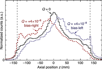
Figure 16. Simulated axial  annihilation distributions [133] for charge Q = 0 (black) and
  under bias-right (red) and bias-left (blue) conditions. The vertical dashed lines locate axial cuts used in ALPHA's analysis of their annihilation vertex data.
Download figure:
Standard image High-resolution image
This technique was applied to data collected over two years, and the observed value of  ,
,  mm, resulted in a limit on the charge of
  (90% confidence). Important systematic effects in this measurement included drift over the long data-taking period (especially because of the weak interleaving of data with different electric field directions), and alignment of various components of the apparatus. Estimates of these have been included in the result for
  quoted above. However, the dominant uncertainty is still the relatively small size of the sample set.
7. Outlook
An outlook for a field as vibrant as antihydrogen physics will necessarily be incomplete, but we can attempt an overview of what measurements can be expected in the near future. Before going into details of these experiments it is, however, important to make a first stop at CERN's antiproton facilities, as they are to be given a significant upgrade in 2017 with the addition of a small deceleration ring called ELENA (extra low energy antiproton ring) [134].
7.1. ELENA
CERN, in collaboration with the AD user community, is building the new small storage and deceleration ring ELENA that will further decelerate the AD antiproton beam from 5.3 MeV to 100 keV [134]. The importance of this extra deceleration stage from a user-perspective is that it will significantly improve the antiproton capture efficiency for all experiments. It is expected that ELENA can decelerate essentially all of the AD beam. Thus, ELENA will deliver a total of ∼3 × 10⁷ antiprotons at 100 keV about every 100 s. The foil-moderator degrading efficiency to the typical ∼keV trapping energies used by most experiments is expected to rise dramatically and to be of order 50%, thus providing an almost 100-fold increase in trapped antiprotons available for further use.
Further, ELENA provides another significant advantage over the AD-only situation. Due to the low energy of ELENA-cooled antiprotons, the extracted beam will be transported by electrostatic, rather than magnetic, beam lines to experiments. This will facilitate rapid bunch-to-bunch switching between experiments. As ELENA is expected to extract four bunches each consisting of close to 107 antiprotons, rapid switching will allow each of these bunches to be sent to separate beamlines, thus ensuring almost continuous access to antiprotons for all experiments.
The nature of the antiproton experiments at CERN is notably different from many of the other CERN experiments (such as those at the LHC) in that most are not (until now) statistics-limited, but more often, development-limited. Development typically requires access to antiprotons in general, therefore, it is not so much the total accumulated number of antiprotons received that is the governing factor for results, but the total time with access to antiprotons. Once operating in a statistics-limited regime, the increased antiproton number has the potential to enhance the rate at which statistically significant results can be achieved. In both respects, ELENA will be a game-changer.
7.2. Microwave spectroscopy
In the realm of probing violations of CPT symmetry in all aspects of antihydrogen physics, ground-state hyperfine spectroscopy offers the possibility of testing CPT in the sub-milli-electronvolt range to high precision. In hydrogen, the best measurements of the ground-state hyperfine transition frequency are made with atomic masers, which interrogate large numbers of hydrogen atoms trapped within a chamber for extended periods of time (see [135] for a review of these techniques.) The most precise measurement to-date has been made in this fashion with a reported transition frequency  of 1420 405 751.7667 ± 0.0009 Hz [43]. It it unlikely that this type of technique could ever be applied to antimatter, however we outline here the main efforts towards approaching this level of precision.
We have summarized earlier (see section 6.1) how ALPHA achieved the first glimpses of the internal structure of antihydrogen by using resonant microwaves to induce a positron spin flip in the ground state anti-atom. Additionally we have briefly described how microwave spectroscopy of the hyperfine structure of antihydrogen is being pursued by the ASACUSA collaboration [119]: see section 5.2.
In the envisaged ASACUSA apparatus, the measurement will be performed in a region of zero magnetic field, effectively eliminating the magnitude of the magnetic field as source of uncertainty, and a precision better than 10−6 [136] is expected. However, the number of antihydrogen atoms available for interrogation is strongly reduced by the small acceptance of their antihydrogen spectroscopy beam-line. Furthermore, only ground state atoms will be useful for spectroscopy. This requirement limits the detection rate, as the antihydrogen atoms are typically created in excited Rydberg states and a significant period is required to relax to the ground state (a time which may be long compared to the flight time to their detector). The ASACUSA collaboration is actively pursuing ways to ensure that cold ground state atoms emerge directly from their antiproton–positron mixing procedure, guided by simulation [120].
The trap-based ALPHA setup guarantees that the nascent antihydrogen atoms have sufficient time to reach the ground state. However the atoms are trapped within an inhomogeneous magnetic field. The effect of this field is to broaden the transition as a result of the atoms' transit through different magnetic fields. The influence of this field can be reduced through a number of approaches. First, as discussed previously, the field has a minimum at the centre which results in the lineshapes of the hyperfine transitions having a relatively sharp cut off below resonance (see figure 14). This effect can be exploited by making a larger volume of the trap at the minimum field through the addition of compensation coils between the main mirror coils. The possibility to achieve this has been built into the recently commissioned ALPHA upgrade [96]. In the spin-flip experiment [113] the magnetic field was measured using electron cyclotron resonance [114], which had an absolute precision of ∼0.2 mT. This can be improved by using an atom or an ion as a magnetometer in order to enhance the precision of the final result.
Finally, in a trap-based method, one may chose to measure the energy difference of the  and
and  states, the antiproton spin flip frequency, rather than that of the positron. This transition has the advantage that at a magnetic field of 0.65 T the frequency is relatively insensitive to magnetic field changes, thus strongly reducing the uncertainty from (lack of) knowledge of the magnetic field [113, 137]. At 0.65 T the
  to
to  transition is around 650 MHz and the weak dependence on magnetic field combined with the recent precision measurement (4.4 × 10⁻⁶) of the antiproton magnetic moment by DiSciacca et al [138] in principle allows a ∼10−6 measurement of the hyperfine splitting in antihydrogen with the current level of experimental control.
7.3. Laser spectroscopy
Spectroscopy of the antihydrogen 1S–2S two photon transition has been a goal for antihydrogen physicists since the idea of making antihydrogen emerged [139, 140]. The fantastic precision with which the equivalent transition in hydrogen is known (currently 4.2 × 10⁻¹⁵ [42]) holds the promise of one of the most precise absolute comparisons of matter and antimatter systems.
The hydrogen measurements were performed in a crossed beam-type setup in a manner that currently seems infeasible for antihydrogen. Spectroscopy on the latter is therefore most likely to be carried out first on trapped anti-atoms. It is notable that the 1S–2S line has also been studied in trapped hydrogen [141]. Trapped atoms pose a number of challenges, not the least of which is the inhomogeneous magnetic field. However, initial precisions of ∼10−10 should be feasible with trapped antihydrogen as demonstrated for hydrogen by Cesar et al [141]. To reach higher precision a number of issues need to be addressed. The trapped hydrogen measurement was limited by laser line-width which is unlikely to be the case for the first antihydrogen experiments. These are, however, likely to be constrained by time-of-flight broadening, as the atoms' motion will cover a large volume of the trap, passing only occasionally and briefly though the laser beam, which is tightly focussed to have sufficient intensity to excite the transition.
While the 1S–2S transition has the potential for the highest absolute precision comparison between matter and antimatter, this may only be released by first addressing the 1S–2P transition that can be used for laser-cooling of the antihydrogen, thereby paving the way to resolve the transit time issue mentioned above. Successful laser-cooling of hydrogen was carried out by Setija et al [142], and should therefore also be feasible for antihydrogen. However, if the cooling laser is directed along only one axis, the weak coupling of transverse and axial degrees of freedom may limit the cooling power achievable [143]. Measuring the 1S–2P transition itself, while not directly on the path to the ultimate precision, could constitute a first measurement in antihydrogen, possibly at the 10−9 level.
7.4. Gravity
The gravitational behaviour of antihydrogen is also the focus of current experimental activity. As mentioned above, two experiments, AEgIS and GBAR, are dedicated to determining the acceleration of antihydrogen due to the Earth's gravity,  . Both of these experiments aim to measure
  in a region free of magnetic field, in a beam (in the case of AEgIS) and at rest (in the case of GBAR). As highlighted above (section 6.2) the ALPHA collaboration recently demonstrated that their sensitive annihilation detection allowed crude limits on the ratio of the inertial and gravitational masses of antihydrogen to be set in their existing apparatus.
The interesting challenge for gravity measurements is the level of environmental control required. Ground state antihydrogen will experience a force equivalent to 1g caused by a magnetic field gradient of only 18 Gm−1. Controlling the environment, or making the experiment insensitive to such stray fields, may be an important challenge for all attempts to probe the gravitational behaviour of antihydrogen. Throughout this review we have discussed several experiments that are aiming to progress this area by at first determining at least the sign of gravity for antimatter, and later improving the measurement limits to the 10% and 1% level (of g) [128, 144]. As these experiments face a number of challenging milestones it is not out of the question that one (or both) of the trapping based experiments (i.e., ALPHA and ATRAP), while not as sensitive in principle, will be able to produce results on a competitive timescale. If the challenges can be met, more exotic schemes have been proposed to take the precision to the 10−6 level using atomic fountain techniques [145].
7.5. Other measurements
While spectroscopy and gravity are of course key directions for antihydrogen research, other measurements can be envisaged that exploit various features of the existing experimental systems. We previously discussed the retrospective analysis by ALPHA that extracted a bound on the neutrality of antihydrogen [133]. In this experiment, the strength of the Coulomb force (on a putative antihydrogen charge) relative to the magnetic confinement of the antihydrogen magnet moment meant that the apparatus was sensitive at a competitive level to existing measurements without special experimental design. It is anticipated that systematic uncertainties in the ALPHA apparatus would ultimately limit the precision achievable by such an approach (quantifying spatial deflection of putatively charged antihydrogen) to a level similar to that reported ( ), even with an increase of measured events. However, other proposals exist to enhance the sensitivity to charge neutrality which would not have the same types of systematic uncertainties (e.g. [146]). It is likely that further tests of the neutrality of antihydrogen are feasible and that such measurements could provide precise (if indirect) measurements of the charge of the positron or the antiproton.
7.6. Limitations
All experiments in antihydrogen physics are currently challenged by the low number of appropriate antihydrogen atoms available. While the ELENA facility will provide more antiprotons, it is likely that the increased number of antiprotons will not trivially translate into larger samples antihydrogen relevant to precision measurements (trapped or otherwise). The anticipated increase in antiproton availability enabled by the ELENA facility will give more time for each experiment with antiprotons, and this, at least initially, seems to be the most significant improvement for experiments. The enhanced antiproton availability is critical to foster the development of new ways to operate with the increased flux, and to optimize the production of cold antihydrogen.
At present, the key issue facing all endeavours is that the antihydrogen needs to be cold for all proposed experiments to work well. For the trap-based activities, it is easy to see why, as only atoms with a temperature ≲1 K can be trapped. However, the AEgIS and ASACUSA experiments also need cryogenic antihydrogen (the former for certainty in the timing and trajectory of antihydrogen along their interferometer, and the latter to increase the probability of measuring ground state atoms with their device).
Much work has been done on making the constituents of antihydrogen cold, as discussed previously in this review, and several methods have been developed to ensure that the antihydrogen is cold when created. However, further progress will be needed to achieve the measurement precisions (i.e., comparable to current limits on hydrogen) that are the ultimate aims of the programmes. One recent proposal by Madsen et al, specifically targeted at the ALPHA experiment, but potentially applicable to others, is to bring a laser-cooled non-neutral plasma of Be+ ions in contact with the positron plasma used to form antihydrogen. The concomitant additional cooling of the positrons, would, according to simulations ([147]), give about an order of magnitude reduction in the temperatures available for antihydrogen formation.
As discussed earlier, antiproton cooling has been demonstrated using evaporative and adiabatic cooling techniques. Work is presently being undertaken to achieve sympathetic laser cooling using osmium anions (e.g. [148]), which could provide a route to ultra-cold antiprotons (<1 mK), and significantly more trapped antihydrogen atoms.
In addition to cooling antihydrogen ingredients further, proposed alternative methods of forming antihydrogen recognize more specifically that the antiprotons carry most of the momentum [78], and therefore aim to keep them cold in the formation process. For example, Ps charge-exchange reactions avoid the problems of merging two plasmas and all their associated electrostatic energy (originally proposed by Deutch, Charlton et al, and discussed in more detail in section 2.3) [69, 70]. The complete hybrid approach is direct formation of antihydrogen ions ( ) and subsequent sympathetic laser cooling with an ion, as proposed by GBAR (section 5.2.3). However, much work remains to validate these methods, including demonstration of useful antihydrogen formation rates and compatibility with precision experiments.
8. Concluding remarks
The trapping of antihydrogen in 2010 and the promise that this holds for antihydrogen physics has led to a flurry of activity in the field—only further fueled by the first observation of a quantum transition in antihydrogen in 2012 and the approval of the ELENA project at CERN that will increase the availability of antiprotons significantly from 2017.
We have reviewed the latest developments in this exciting field and given some historical background with emphasis on the lines of research that have borne fruit at this point in time, while keeping in mind a number of parallel developments that may become important for the future. This includes the results above, but also techniques novel to the field such as evaporative cooling, adiabatic cooling and autoresonant manipulations. We have further tried to give an overview of the directions of current and near-future efforts that can be roughly split in the groups that start their experiments from trapped antihydrogen and those that plan to make antihydrogen directly in low-energy beams to avoid the issues related to the magnetic fields required for trapping.
With a total of four active antihydrogen experiments at CERN and one more under construction, we can look forward to many interesting results in the coming years. We therefore anticipate that antihydrogen will soon live up to its promise as one of the foremost testbeds for fundamental physics at low energies.
Acknowledgments
We thank our colleagues in the ALPHA collaboration, the AD operations team and the wider antiproton physics community for decades of effort that have led to the state of the field today. The authors would like to acknowledge EPSRC, the Leverhulme Trust and the Royal Society for funding their research.