
Abstract
Simulations have been performed of the radial transport of antiprotons in positron plasmas under ambient conditions typical of those used in antihydrogen formation experiments. The parameter range explored includes several positron densities and temperatures, as well as two different magnetic fields (1 and 3 T). Computations were also performed in which the antihydrogen formation process was artificially suppressed in order to isolate its role from other collisional sources of transport. The results show that, at the lowest positron plasma temperatures, repeated cycles of antihydrogen formation and destruction are the dominant source of radial (cross magnetic field) transport, and that the phenomenon is an example of anomalous diffusion.
Export citation and abstract BibTeX RIS

Original content from this work may be used under the terms of the Creative Commons Attribution 3.0 licence. Any further distribution of this work must maintain attribution to the author(s) and the title of the work, journal citation and DOI.
1. Introduction
Recent years have seen many advances in studies with antihydrogen,  . These have included: the first formation experiments involving the controlled mixing of antiprotons and positrons [1, 2]; the successful trapping of small samples of the anti-atoms in magnetic minimum neutral atom traps [3–6]; the demonstration of beam-like propagation of antihydrogen [7, 8] and the first explorations of its properties [9–12]. This work was undertaken at the unique Antiproton Decelerator facility located at CERN [13, 14] which supplies pulses of 5.3 MeV antiprotons (
 ) every 100 s or so for subsequent experimentation.
One of the basic instruments used for almost all antihydrogen experiments to date is the Penning, or Penning–Malmberg, trap. These are examples of charged particle traps (see e.g., [15–17]) which are used to collect, control and manipulate  and positron (e+) clouds and plasmas, and to mix them to form the anti-atoms. Such traps employ strong magnetic fields (typically of tesla strength) for radial confinement of the charged species, as the field is directed along the axis of a series of electrodes, with the latter suitably electrically biased to provide the axial confinement. To date, almost all antihydrogen experiments have involved mixing antiprotons and positrons in a so-called nested Penning trap environment [18] in which typical e+ cloud/plasma temperatures, Te, have been below 100 K (though this parameter was not always directly measured) and with densities in the range from ne = 1013–1015 m−3. It has been found that antihydrogen is typically formed via the three-body interaction given by

It has been well-documented how the nascent anti-atoms are very weakly bound (by of the order of  for reaction (1) [19–21], where their excited nature is denoted by the double-star superscript), and are thus susceptible to influence from the local fields, and in particular the trap electric field, and the e+ plasma self-field. The influence of these has been observed in several experiments in which field ionisation of the anti-atoms has resulted in
  separation from the e+ plasma [22, 23], and has also been exploited as a means of probing antihydrogen formation and to gain insight into binding energies [2, 7, 8, 24].
The weakly bound newly formed antihydrogen atoms may also be affected by collisions in the e+ plasma: indeed, it has been emphasised elsewhere, and in particular in [21], how the antihydrogen that is detected is a result of a detailed sequence of processes which involve repeated cycles of antihydrogen formation according to reaction (1), and break-up in collision as

This process is likely to have a very large cross section, probably in excess of geometric (∼10−12 m−2), leading to collision frequencies for ne = 1014 m−3 of around 107 s−1, which is much faster than the inverse of the time taken for an antihydrogen atom to travel 1 mm (about 1 μs). This reaction will also be in competition with de-excitation of the  ,
,

which may lead to a state stable against subsequent ionisation. The overall equilibrium rate for the production of stable anti-atoms through three-body recombination (1) and subsequent collisional stabilisation (3) is proportional to  (see e.g., [19, 25, 26] for further discussion). (Note that radiative recombination is an alternative route to
  formation and is expected to preferentially produce low-lying, deeply bound states at low rate: see e.g., [25]. This process will deplete the
  cloud, but will not otherwise disturb it, nor the positron plasma, and it is therefore not included in the discussion here.)
Following the initial ATHENA and ATRAP experiments [1, 2, 22, 24, 27–30] a number of authors undertook simulations and theoretical analyses of various aspects of antihydrogen formation, as applied to the experimental situations [31–41], and as summarised by Robicheaux [20].
In this spirit, a detailed examination of antihydrogen formation was undertaken by Jonsell et al [21] under simulated conditions appropriate to those of the ATHENA experiment, and the present work is in part based upon some of their observations. They found that the fraction of time that an antiproton spends bound as antihydrogen is usually small, typically less than 1% (at Te = 15 K and ne up to 1015 m−3). This was interpreted as being due to the rate of the two-body destruction process, reaction (2), greatly exceeding that for the three-body formation rate of reaction (1), due to, as mentioned above, the very large cross section for break-up. Furthermore, they found that the radial distributions of the antiprotons were time-dependent. This was attributed to cross-magnetic field drift of the  while neutralised as antihydrogen, before break-up, but with the latter occurring at a larger (on average) radius, r (with r = 0 the z- and B-field axis of the system) than the formation event.
Thus, as time proceeds during a e+– mixing experiment, the antiprotons progressively move towards the outer edge of the positron plasma. The importance of this is that here the combination of the plasma self electric field
  (which is radial,
  , in nature with e the elementary charge and
  the permittivity of free space) and the uniform axial magnetic field,
  , provided in the experiment by a solenoid results in an antiproton tangential speed given by
  , proportional to the radial position of the
  . As an example, take r = 1 mm, B = 1 T and
  m−3, to find vT ∼ 900 ms−1, which corresponds to an effective temperature/equivalent kinetic energy of around 33 K. This is to be compared to typical antihydrogen trap depths, which are around 0.5 K. Thus, it is clear that if antihydrogen is formed in dense positron plasmas the radial position of creation will have a direct bearing on the ability to trap the anti-atom for further study.
Motivated by the results of the earlier simulations [21], and the importance to the aforementioned experiments involving antihydrogen trapping and also to the creation of beams of (ground state) anti-atoms for hyperfine spectroscopy, we have performed a more detailed study of  radial transport in dense, cold e+ plasmas during antihydrogen formation. We have explored the positron density range from 1013–1015 m−3, with positron temperatures between 10 and 50 K, and for applied magnetic fields of 1 and 3 T. The higher ne and B are typical of early experiments (e.g,. ATHENA [1, 22, 30]) for which there are data to which semi-quantitative comparisons can be made. More recently lower B fields have been used to help promote
  capture in magnetic minimum traps, typically alongside lower ne which has been found to be helpful in the quest for lower
  temperatures.
The methodology we have adopted is described in section 2, with our results and discussion presented in section 3. We draw our conclusions in section 4.
2. Simulation methodology
The simulations were performed using the methodology developed, and described fully, by Jonsell et al [21]: thus, we need only provide a brief summary here. The  trajectories were computed using classical equations of motion, along with those of any e+s within a cylinder of radius and height
  . The use of classical equations is valid since quantum mechanical effects are only relevant on much smaller length scales than those of the typical e+–
 interactions under the plasma conditions considered here. The particle trajectories were found by integrating Newton's equations of motion for the Lorentz force
  , where, as above, B is a uniform solenoid field (i.e., we do not attempt to model the situation in which an additional non-uniform magnetic field is applied to confine some of the anti-atoms, though this will typically be a minor perturbation due to the small plasma size relative to the atom trap). In this work we focus on the motion of antiprotons inside the positron plasma, where the electric field is the plasma self electric field (
 , as defined above) and has no axial component. The number of trajectories was usually 20 000 for each parameter setting.
Since this study does not seek to simulate experimental procedures, which typically involve various means of injecting the antiprotons into the positron plasma, the antiproton trajectories were initialised at zero radius, with a thermal velocity distribution (set by Te) in the radial and axial directions. Our simulation distinguishes free antiprotons from those bound inside an antihydrogen atom. In the former case the charged particle is subject to a drag force from the plasma [42], as well as a diffusive force related to the drag by the fluctuation dissipation theorem. While bound as a neutral antihydrogen atom the antiproton is not subject to these forces, and instead the interaction with the one or more positrons present is calculated explicitly. This procedure necessitates a clear distinction between bound states and continuum states of any positrons in the vicinity of the antiproton. In the presence of strong magnetic and electric fields typical of antihydrogen experiments, this separation is not well defined. Thus, in our simulations we calculate large numbers of many-positron antiproton collisions and any collision ending with a positron bound to an antiproton by more than  (the binding energy calculated without including external electric and magnetic fields) is defined as formation of an antihydrogen atom. The rate of such events is evaluated (see table 2), and the positron state after the collision is saved as the initial condition for an antihydrogen atom.
Table 1.
Exponents of large  jump size distributions
  .
.
| Te (K) | ne (m−3) | B (T) | n |
|---|---|---|---|
| 15 | 1015 | 1 | 2.0 |
| 15 | 1015 | 3 | 1.9 |
| 30 | 1015 | 1 | 1.7 |
| 30 | 1015 | 3 | 1.7 |
| 15 | 5 × 10¹⁴ | 1 | 1.6 |
| 15 | 1014 | 1 | 0.9 |
| 15 | 5 × 10¹³ | 1 | 1.0 |
Table 2.
The frequency,  , of antihydrogen formation events in the plasma. A formation event is defined as a three-body collision which results in a
  state with binding energy (calculated without including the external fields) larger than
  , where Te is the plasma temperature.
| Te (K) | ne (m−3) | B (T) |
 (s−1) (s−1) |
|---|---|---|---|
| 15 | 1015 | 1 | 9.7 × 10⁴ |
| 30 | 1015 | 1 | 5.0 × 10³ |
| 10 | 1015 | 3 | 4.8 × 10⁵ |
| 15 | 1015 | 3 | 8.2 × 10⁴ |
| 20 | 1015 | 3 | 2.4 × 10⁴ |
| 25 | 1015 | 3 | 9.2 × 10³ |
| 30 | 1015 | 3 | 4.2 × 10³ |
| 50 | 1015 | 3 | 4.8 × 10² |
Our main observable is the radial position of the antiproton, as a function of time. We can also track other quantities such as the change in radial position, Δr, of each jump, the binding energy of the antihydrogen formed etc. We can vary external conditions such as plasma temperature, density (and hence electric field) and magnetic field.
3. Results and discussion
Though our simulations assume that the positrons and antiprotons are in thermal equilibrium, the nature of the  formation and break-up cycles (reactions (1) and (2)) mean that the rate of stable (against break-up, say via reaction (3), and which might thus be observed by experiment)
  production and the transient rate of
  formation in the positron plasma, are not the same. It is expected that the latter will be much higher than the former, and they will not necessarily have the same dependence upon Te. In the analysis presented after the discussion of the simulation results, we attempt to estimate the overall rates of
  production and break-up in the positron plasma, as it is these that, under circumstances elucidated by the present study, can govern the cross-field transport of the antiprotons.
When a neutral antihydrogen atom is formed its centre-of-mass motion will cease to be influenced by the electric and magnetic fields in the plasma, though its momentum vector will be dominated by that of the antiproton at the moment of antihydrogen formation. The antihydrogen will continue largely in the same direction until it is again ionised, and the  resumes its circular motion around the axis of the trap. It will, however, now circulate at a different trap radius because of the motion it made while bound as antihydrogen. Thus, an antiproton will make a radial 'jump'
  every time it is bound transiently as an antihydrogen atom.
The size of these 'jumps' will follow some distribution  . Examples of our simulated results for such distributions are shown in figure 1. If the motion of the
  were only due to thermal effects, one would expect a
  distribution symmetric around
  . In contrast, if the radial drift were only due to the tangential velocity component arising from the
  drift motion one would always have
  . Hence, the combination of these two effects gives a distribution with both negative and positive
  , but with a bias towards positive jumps. This will be discussed in more detail below.

Figure 1. Distribution of changes in radial position  of an antiproton between the times of formation and ionisation of an antihydrogen atom. Temperature Te = 15 K, density ne = 1015 m−3, and magnetic fields B = 1 T (black) and 3 T (red). The inset shows the large
  tails on a log–log scale, including fits to a distribution
  , where n = 2.0 for B = 1 T and n = 1.9 for 3 T.
Download figure:
Standard image High-resolution imageConsidering radial motion due to antihydrogen formation only, starting from r = 0, the radial position at some later time, tN, will be the sum of all N jumps,  . The time required to make N jumps is on average given by N divided by the antihydrogen formation rate
  increased by the time the
  spends as an
  ,
,  . Hence, the average radial
  speed due to antihydrogen formation is given by
where  (with
(with  ) is the fraction of time the
  spends as
  . The average
  can also be written as

where r0 is the radial position before the jump.
It is therefore interesting to study how the distribution  falls off for long
  (see the inset of figure 1). The large
  tail of the distribution will, through the influence of Δt, have a very complicated dependence on the binding energies of the
  formed, and how the binding energy evolves as the
  undergoes further collisions. We find this behaviour by fitting to simulated data, such that the tail is well described by a power law
  , with
  for different parameters (see table 1). Our data indicate that the distribution falls off more slowly at small densities, which can be expected, as at higher densities the collision frequency is higher, and thus Δt shorter. In fact, due to the slow fall off the integral in (5) diverges, as is characteristic for anomalous diffusion influenced by Lévy flights [43]. This necessitates a cut-off in the
  distribution, which we will discuss further.
In addition to the change in radial position when neutral as  , there is also, as explained in section 2, diffusive drift of the bare
  . Considering this drift alone, we can write the diffusion as a series of small jumps in the x- and y-directions:
  with zero average
  . Note, that these displacements are relative the bulk motion of the plasma, i.e. take place in a reference frame rotating with the
  drift velocity of the positron plasma. Looking at the mean square radial displacement
where the average of  and
and  is
is  . Since we here consider only the thermal drift, which is made up of much more frequent and smaller jumps (as compared to the radial jumps induced by antihydrogen formation), we consider this as a continuous process, relating the number of jumps to time t, through N = λept, where λep is the positron–antiproton collision frequency. We can also define the usual diffusion coefficient D through
  . We will return to this below.
The magnetic field dependence of the collision frequency, as well as of the jump size distribution, is not dramatic, leading to a similar rate of radial transport for different field strengths. The antihydrogen formation rate is, however, reduced by a factor of around 20 when the temperature is doubled from 15 to 30 K: see table 2. This, coupled to a not too different jump-size distribution, gives a dramatically reduced rate of radial transport as the temperature is increased. In fact, at higher temperatures normal thermal drift dominates.
The slow fall off for large  in figure 1 makes the radial position of the antiprotons, when averaged over many trajectories, very sensitive to a small number of trajectories involving very large radial jumps. This makes the average difficult to calculate, or even undefined. We therefore need to introduce a cut-off radius rc = 1 mm, removing any antiprotons which cross this radius from the average. This is physically motivated by the finite radius of any real positron plasma (assuming that the antihydrogen is field-ionised outside the plasma, or that any remaining radial transport outside the plasma is not interesting for our purposes). As a consequence, when radial transport is significant, the average will approach, but never cross rc. At the same time the average will be taken over a decreasing number of trajectories (since some are removed because they crossed the cut-off radius), leading to increasing statistical fluctuations. This cut-off changes the upper limit of the integral in (5) to
  making the average
  and the attendant speed
  well defined.
An example of the time evolution of the radial distribution of antiprotons is shown in figure 2. It can be seen that at short times most antiprotons are located well within the plasma (i.e. at r < rc = 1 mm). As time progresses the peak of the distribution grows outwards. The distribution is sharply cut off at r = rc, representing the outer radius of the positron plasma. The tail extending beyond rc is removed from the simulation, with the effect that the integral of the distribution with time diminishes from its initial value 1.0, until in the end all antiprotons would have left the plasma (at 0.2 ms the integral is 0.7, while at 1.0 ms it is 0.12).
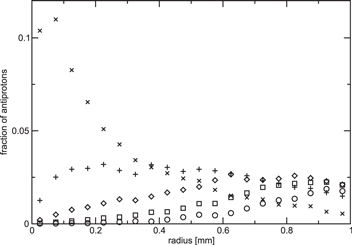
Figure 2. Time evolution of the average radial position of the antiprotons for ne = 1015 m−3, B = 3 T and Te = 15 K. The symbols represent different times, 0.2 ms (×), 0.4 ms (+), 0.6 ms ( ), 0.8 ms (□), and 1.0 ms (○). In the simulation 20000 antiprotons were initiated at r = 0. Note that the distribution is cut off at rc = 1 mm (see text).
Download figure:
Standard image High-resolution imageThe results of our simulations for various densities, temperatures and magnetic fields are shown in figure 3, and can be contrasted with those shown in figure 4, where antihydrogen formation was artificially turned off. The radial drift is then exclusively due to thermal Brownian motion, which is confirmed by good fits to  , when thermal diffusion is slow (we attribute the deviation from the linear dependence when the diffusion is fast to the velocity-dependence of the friction coefficients from [42], and the difference at large positron densities between the drift velocity of the e+s and the
  [21]). Here, the effect of the magnetic field is more important than the temperature, since it pins the charged particles to field lines, thus inhibiting radial motion.

Figure 3. Time evolution of the average radial position of the antiproton, assuming a plasma radius of rc = 1 mm. The values for the plasma temperature Te and the magnetic field B are indicated in each panel. The symbols represent different plasma densities, from above ne = 1015 m−3 (×), ne = 5 × 10¹⁴ m−3 (+), ne = 1014 m−3  , ne = 5 × 10¹³ m−3 (□), and ne = 1013 m−3 (○).
Download figure:
Standard image High-resolution image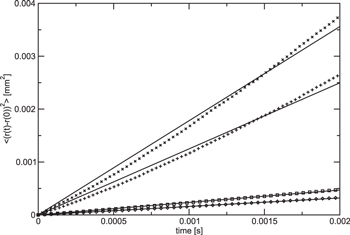
Figure 4. Time evolution of the average radial position of the antiproton, excluding the effects of antihydrogen formation. Here ne = 1015 m−3, and Te = 30 K, B = 1 T (×), Te = 15 K, B = 1 T (+), Te = 30 K, B = 3 T (□), and Te = 15 K, B = 3 T  . The lines are fits to
  , as is characteristic for thermal Brownian motion.
Download figure:
Standard image High-resolution imageThe temperature dependence of the radial drift is examined in figure 5. As expected the radial drift is much slower at higher temperatures. We find that the drift varies sharply with the temperature of the positrons; at 10 K all simulated trajectories have crossed rc within 1 ms. Increasing the temperature by only 5 K there are still antiprotons remaining up to 2 ms, but a significant fraction have left the plasma, as is visible by the trend towards saturation at rc. At 50 K more than 90% of the antiprotons remain after 2 ms, but a small fraction has jumped by large Δr and either left the plasma or contributed to raising the average  significantly compared to thermal-only diffusion.
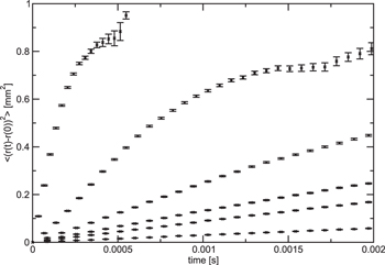
Figure 5. Change in average radial position,  of the antiprotons as a function of time and for different temperatures. The data are for 10, 15, 20, 25, 30 and 50 K with the upper curve being that for the lowest temperature, and with the remainder in order of increasing Te. In all cases ne = 1015 m−3 and B = 3 T. The error bars show the standard error of the mean.
Download figure:
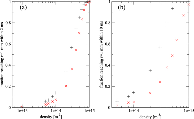
Standard image High-resolution imageAn experimentally relevant measure of the rate of radial antiproton drift is the fraction of antiprotons reaching the outer radius of the plasma, within a certain time. We plot this fraction after 2 ms as a function of density and magnetic field for a 15 K plasma in figure 6(a), which shows that it rises rapidly above about ne = 1014 m−3 due to the influence of  formation by reaction (1). Again, the dependence on magnetic field is weak. In a 30 K plasma the time scale for the antiprotons to reach rc is longer. For this temperature, and in the density range investigated, we have to wait between 0.01–0.1 s, to find a significant fraction of antiprotons at this radius, as can be seen in figure 6(b). At 15 K the antiproton radial drift contributes little, confirming that a mechanism involving the formation of antihydrogen is the dominant reason for radial transport.
Figure 6. (a) Fraction of antiprotons reaching r = 1 mm, within 2 ms as a function of density for a Te = 15 K plasma and B = 1 T (black, +) and 3 T (red, ×), (b) same but Te = 30 K and waiting time 10 ms.
Download figure:
Standard image High-resolution image
In what follows, an attempt is made to develop a simple model of the transport of antiprotons in positron plasmas in an effort to underpin the results of the simulations. Combining the ballistic diffusion with speed  from (4), with the normal diffusion during the time
  the
the  is free, we find
where  is the positron–antiproton collision frequency and in which we have assumed that
  : see below. The average time required for the
  to diffuse out to some radius r is then
There are two limits, (i) when  ballistic diffusion dominates and
  and (ii) in the opposite limit thermal diffusion dominates and
 ![$t\simeq {r}^{2}/[(1-{F}_{\bar{{\rm{H}}}}){\lambda }_{\mathrm{ep}}\langle {\rm{\Delta }}{r}_{\bar{p}}^{2}\rangle ]$](https://content.cld.iop.org/journals/0953-4075/49/13/134004/revision1/jpbaa25d0ieqn99.gif) . The relative importance of the two effects can be parameterised by the ratio
. The relative importance of the two effects can be parameterised by the ratio

We now estimate the size of the  radial step in a collision with a positron. Positrons in the plasma have a speed
  (since positrons are pinned to magnetic field lines we use the average of the one-dimensional Maxwell-Boltzmann distribution). Using momentum conservation we expect that
  . Further using
  , with Ωc = e B/M the cyclotron frequency of the antiprotons, we find that
It is now assumed that the positron–antiproton collision frequency is given by  , with ne the positron density and
  is the classical distance of closest approach. Here collisional suppression effects due to the presence of the strong B-field have been ignored. It can then be shown that
The rate of cross-field transport (as an antiproton, distinct from antihydrogen) is proportional to  , which can be written from (10) and (11) as

This naive estimate contains no plasma effects. Comparing to the full treatment in [42] we find, within the relevant parameter range, an approximate agreement if  is multiplied by the dimensionless parameter
  , where
  is the Debye length of the plasma, and
  is a high momentum/short distance cut off. (Note that ξ varies from 1–3 over the full parameter range explored in this work.) Here we take
  . Thus we find
where

Inserting values for the constants it is found that  , which for B = 3 T, ne = 1015 m−3 and Te = 15 K yields
  , which is roughly comparable to the result from the simulation (see figure 4). Further, the scalings with Te and B also roughly agree with the results in figure 4.
The next step is to estimate the size of the jumps made as antihydrogen, which is taken to be the thermal  speed (which is assumed to be that of the antiproton), multiplied by its time of flight before destruction in collision. Thus we can write

with  the break-up collision frequency, where
  is some average break-up cross section for the highly excited states of antihydrogen that exist fleetingly in the plasma. Putting numbers (
 m−3 and
  m2) into (15) we find
  m. This is comparable to the average of
  in figure 1 (when, as discussed above, only
  mm are included in the average). This shows that our estimate for
  is reasonable. However, the thermal velocity will be isotropic, and thus give rise to a
  which is symmetric around zero, i.e.
  . This gives only a contribution to diffusion, which we neglect compared to the diffusion of the
  in their bare state, that is, we ignore the fluctuations in the
  transport, and hence approximate
  .
.
The net outward drift is instead given by the rotational  drift velocity of the
  (introduced in section 1), which upon formation is transferred to the
  as a tangential velocity
  , where we take
  to be the direction tangential to the
  motion at the time t = t0 of formation (here r0 = r(t0)). This means that
  . The total velocity is then
  , where
  is the thermal velocity in the i-direction, which averages to zero. As such, the change in radial position is given by
  where
where  is the time between formation and ionisation. For short jumps
  one has
  , and hence
  . In the opposite limit
  , that is linear in Δt, and
  . Since
  the product vTΔt is independent of positron density, and we expect
  to be largely independent of density for large
  . For relevant parameters (B = 3 T, ne = 1015 m−3 and T = 15 K) we find that the long jumps should give the dominating contribution to the
  transport, a result which is confirmed by simulations.
We now write the formation rate for the three-body reaction in terms of ne and Te as  , where for the moment the Te dependence is parameterised in terms of the exponent, k, noting that k = 4.5 applies in equilibrium for the production of antihydrogen bound deeply enough to survive further collision. From this it is easy to show, after a little substitution, that

This is likely to drop rapidly with Te. (Here it is assumed that the break-up cross section is independent of the plasma parameters, but this may not be true, due to the nature of the weakly bound states.)
We now perform a crude estimate of  . It would be possible to use the zero-field equilibrium three-body coefficient for
  : as a result the value k = 4.5 would apply. However, as noted above, this is the rate applicable for the formation of antihydrogen that is bound deeply enough to survive further collisions, which is not the case here. It is, however, possible to use the data generated from the simulations at ne = 1015 m−3 to find values for
  and k for the 'in plasma' case (see table 2). These turn out to be C'' = 10−20 m6 s−1 K4.3 and k = 4.3. Thus at ne = 1015 m−3 and Te = 15 K, B = 3 T,
  and assuming
  m−2 (there is evidence that the initial states are of micron size [33, 44], hence this estimate) it is found that
  m s−1, which is of the same order of magnitude as observed in simulations.
We can now also estimate the fraction of time the  is bound inside a
  . From (4)

For the parameters used above  , and we shall therefore approximate
  . This is consistent with [21], where it was stated that the antiprotons only spend about 1% of their time as antihydrogen. Furthermore, from (9), (13), (14) and (16) R can be represented as
Inserting numbers for  and using the above value for
  m−2, r = 1 mm as in our simulations, and
  we find that
  T−1 m4
  . Using B = 3 T, ne = 1015 m−3 and T = 15 K, we find that R ∼ 9.7 × 10⁴, i.e. the radial transport is totally dominated by antihydrogen formation. It is interesting to note that at very early times (small r) thermal diffusion will dominate; that is, if the
  originate on the trap axis there will initially be no transport due to the antihydrogen formation process, because vT = 0. For the parameters above thermal transport dominates while r ≲ 5 μm. In a real experiment, unless antiproton injection is restricted to such a narrow radius, transport due to antihydrogen formation will dominate at all times.
Varying the parameters, the roles may be reversed. For instance still at B = 3 T and ne = 1015 m−3 thermal transport will dominate for Te ≳ 130 K. Reducing the density to ne = 1013 m−3 and the magnetic field to B = 1 T, thermal diffusion dominates for Te ≳ 35 K. According to our simulations, at this density thermal diffusion dominates already at Te = 15 K. However, given the crudeness of our estimate, we conclude that it is in fair agreement with our numerical results. In particular, we expect the very sharp dependence on temperature to be correct.
4. Concluding remarks
We have identified a mechanism for radial antiproton transport in magnetised positron plasmas: namely the repeated formation and ionisation of antihydrogen atoms. We show through simulations that this is the dominant radial transport process within most of the parameter range relevant for current experiments. We also provide a simple model for the relative rate of antiproton transport both through antihydrogen formation, and through thermal diffusion. This model predicts a sharp dependence on temperature of the relative rates, which is consistent with the results from our simulations.
The most recent experiments, where positron densities close to the lower end of the parameter range used in our simulations are typically used [3–12], may be operating in a region where the thermal and  formation mechanisms are comparable in magnitude. If this is the case, then as Te is further reduced, which is a major goal of the current experiments, radial antiproton transport is likely to increase sharply. Further work will include investigating the latter at higher densities, such as those suggested in [45], where we expect qualitatively new features arising from the mismatch between the drift velocities of the antiprotons and the positrons.
Acknowledgments
This research was supported by the EPSRC (UK) and the Swedish Research Council (VR).