


Abstract
Geodesy, the oldest science, has become an important discipline in the geosciences, in large part by enhancing Global Positioning System (GPS) capabilities over the last 35 years well beyond the satellite constellation's original design. The ability of GPS geodesy to estimate 3D positions with millimeter-level precision with respect to a global terrestrial reference frame has contributed to significant advances in geophysics, seismology, atmospheric science, hydrology, and natural hazard science. Monitoring the changes in the positions or trajectories of GPS instruments on the Earth's land and water surfaces, in the atmosphere, or in space, is important for both theory and applications, from an improved understanding of tectonic and magmatic processes to developing systems for mitigating the impact of natural hazards on society and the environment. Besides accurate positioning, all disturbances in the propagation of the transmitted GPS radio signals from satellite to receiver are mined for information, from troposphere and ionosphere delays for weather, climate, and natural hazard applications, to disturbances in the signals due to multipath reflections from the solid ground, water, and ice for environmental applications. We review the relevant concepts of geodetic theory, data analysis, and physical modeling for a myriad of processes at multiple spatial and temporal scales, and discuss the extensive global infrastructure that has been built to support GPS geodesy consisting of thousands of continuously operating stations. We also discuss the integration of heterogeneous and complementary data sets from geodesy, seismology, and geology, focusing on crustal deformation applications and early warning systems for natural hazards.
Export citation and abstract BibTeX RIS
Corresponding Editor Michael Bevis
1. Introduction
Global positioning system (GPS) geodesy deploys precision instruments (GPS receivers and antennas) on platforms, static or dynamic, on the Earth's land and water surfaces, in the atmosphere or in space, to observe the constellation of GPS satellites and to explore a wide range of physical processes in the Earth system. One of the goals is to obtain precise estimates of 3D positions and their displacements in space and time in the case of quasi-static platforms and trajectories in the case of dynamic platforms, although the distinction is somewhat arbitrary. The underlying physical processes of interest may have temporal scales ranging from fractions of seconds (e.g. seismology) to millions of years (e.g. tectonic plate motion) and spatial scales from several meters (e.g. individual geologic faults) to global (e.g. polar motion). One of the advantages of the GPS is that, compared to other measurement systems in geodesy and seismology, it provides positions with respect to a global terrestrial reference frame. Besides precise measurement of point positions and their changes over time that are indicative of dynamic surficial and subsurface processes, all disturbances in the propagation of the transmitted GPS signal from satellite to receiver including troposphere and ionosphere refraction, receiver multipath, and the reflections of signals on solid ground, water and ice may be mined for physical signals. In this review, we emphasize the stringent positioning accuracy requirements of GPS geodesy that differentiates it from the ubiquitous use of GPS in everyday life (e.g. smart phone mapping applications, vehicle navigation). Regardless of the parameter of interest or the temporal resolution, GPS geodesy is defined by the requirement to estimate 3D platform trajectories with millimeter to centimeter-level precision; by comparison, most personal and commercial navigation and mapping applications of the GPS only require meter-level precision.
This review concentrates on applications that benefit from the considerable database of precise observations collected over the last 35 years, as well as more recent and novel applications. The focus is the role that the GPS is playing in improving our current knowledge of the dynamic Earth, as well as how this knowledge can be used to address hazards with significant societal impact. We selectively include equations, graphics, and videos to better demonstrate concepts, rather than providing a textbook-like review. Appropriate historical references provide a cursory overview of other geodetic methods, modern as well as historical. The combination of GPS observations with other types of data from geodesy, seismology, and geology, is dealt with in greater detail. We also discuss outstanding problems in the geosciences, where improvements in GPS and the availability of other emerging satellite constellations will be of benefit. Note that the general class of satellite constellations is referred to as Global Navigation Satellite Systems (GNSS); as more navigation systems become available 'GPS geodesy' and 'GNSS geodesy' are being used interchangeably.
There are several review articles, books, and reports that may be of interest: Theoretical and technical aspects of the GPS and geodetic theory (Hofmann-Wellenhof 1993, Leick 2004, Parkinson et al 1996, Teunissen and Kleusberg 1998, Hofmann-Wellenhof et al 2007, Misra and Enge 2006, Blewitt 2007), tectonic geodesy (Segall and Davis 1997, Bürgmann and Thatcher 2013), seafloor geodesy (Bürgmann and Chadwell 2014), volcano geodesy (Dzurisin 2006, Segall 2010), international conventions for GPS data analysis (Petit and Luzum 2010), and grand challenges facing geodesy (Davis et al 2012a).
To put this review into perspective and to highlight the significant contributions of GPS geodesy to society, we discuss its impact within the context of several recent global scale catastrophes. In a little over a decade the world has witnessed a terrible number of casualties and severe economic disruption from several recent great subduction-zone earthquakes and tsunamis. Two events that we frequently cite in this review are the 26 December, 2004 Mw 9.3 Sumatra–Andaman event that resulted in over 250 000 casualties, the majority of them on the nearby Sumatra, Indonesia mainland with tsunami inundation heights of up to 30 m (Paris et al 2007) and the March 11, 2011 Mw 9.0 Tohoku-oki (Great Japan) earthquake, which generated a tsunami with inundation heights as high as 40 m resulting in over 18 000 casualties (Mimura et al 2011, Mori et al 2012, Yun and Hamada 2014).
2. GPS overview
2.1. Constellation and signals
The global positioning system is a satellite constellation operated by the United States Department of Defense (Air Force) to support military and civilian positioning, navigation, and timing. The first satellite was launched in 1978 with multiple generations of satellites thereafter. The orbital periods are approximately 12 h, so that the satellites are visible over the same ground point about every 24 h. Currently there are 32 satellites in operation in 6 orbital planes. There are at least five satellites visible to support instantaneous positioning at any geographic location, and often there are up to 12 satellites visible. Standard civilian applications require the observation of signal propagation time (expressed in terms of equivalent range or distance) from at least four satellites in order to triangulate the 3D position of the user and to estimate a clock/timing bias; additional observations provide redundancy and estimates of position uncertainties.
Atomic clocks on the satellites produce the fundamental radio frequency of 10.23 MHz and the satellites transmit at integer multiples (154 and 120) of this frequency at two frequencies called L1 (1575.42 MHz) and L2 (1226.60 MHz). Since the ionospheric effects on the signal are dispersive and inversely proportional to frequency, first-order effects on the propagated signal can be canceled by means of a simple linear combination of L1 and L2 observations.
A pseudorange measurement is derived from the measured travel time between a particular satellite and a GPS instrument, biased by instability in the satellite and receiver clocks, hence 'pseudo' range. There are two types of pseudorange codes that are modulated onto the L1 and L2 signals. The precision (P-) code originally intended for military applications is at the fundamental frequency of 10.23 MHz (an effective wavelength of ~30 m) and is modulated onto both the L1 and L2 signals. The P-code is encrypted by the US military (called anti-spoofing) to avoid jamming by adversaries in times of war. The Coarse Acquisition (C/A) code originally intended for civilian users at a tenth of the fundamental frequency (an effective wavelength of ~300 m) was originally only modulated onto the L1 signal, the intent being to limit the stand-alone point positioning accuracy of civilian users by precluding the ionospheric correction, increasing the effective wavelength, and distorting ('dithering') the satellite clock frequency (called selective availability or SA). SA was an intentional degradation of public GPS signals implemented for national security reasons but was discontinued in May 2000 to support civilian and commercial users; it was announced in September 2007 that the newest generation of satellites (GPS III) will not have the SA feature. Furthermore, as stated in the US Government GPS website 'The United States has no intent to ever use Selective Availability again'. Also modulated onto the L1 signal is the broadcast ephemeris message, which includes a description of the satellite orbit at any point in time (orbital elements), timing information, and atmospheric propagation models. The transmissions are maintained by the US Air Force's GPS Ground Control Segment. Consumer devices such as smart phones and vehicle navigation systems only track the C/A code on L1, which limits precision to the several meter level. The precision can be significantly improved to about a meter by using, where available, differential corrections via satellite-based augmentation systems (Van Diggelen 2009).
The GPS is in the process of modernization with the addition of civilian and military signals. Modernized GPS satellites will include four civilian signals. In addition to the C/A signal at L1 (1575.42 MHz) there is a new L2C signal at L2 (1227.6 MHz) allowing for redundancy and ionospheric corrections for users with C/A code receivers. Another new signal L1C at L1 frequency will be available with the latest generation of GPS satellites (Block III) designed to be backwards compatible with the original L1 C/A code signal and with signals from the European Union satellite constellation, Galileo. The United States Air Force began broadcasting pre-operational L2C and L5 civil navigation (CNAV) messages from a few satellites beginning in April 2014. Another broadband civil signal for 'safety of life' aviation applications will be broadcast at L5 (1176.45 MHz). At the time of this writing (August, 2015), there are 17 L2C-enabled satellites and nine L5-transmitting satellites. The US government intends to have 24 satellites broadcasting the L2C signal by 2018 and the L5 signal by 2024. The military M-code for more secure access includes two new encrypted P(Y) signals transmitted at both L1 and L2. The impact of GPS modernization on geodesy will be significant by allowing a new generation of geodetic-quality receivers to replace the proprietary codeless and semi-codeless receivers developed since the 1980s to circumvent P-code civilian restrictions. Furthermore, the addition of a third frequency will provide more accurate, robust, and efficient positioning, in particular for real-time geodetic applications (Hatch et al 2000, Geng and Bock 2013). Observations of other GNSS constellations (e.g. GLONASS, Russia; Galileo, European Union; BeiDou, China) will also have a similar impact through super redundancy and the number of visible satellites, providing improved positioning in urban and other environments with limited satellite visibility. GLONASS has been fully operational since 2012 and is increasingly being used for geodetic, precise surveying, and engineering applications.
2.2. GPS infrastructure and surveys
GPS geodesy was born when it was realized early on in the implementation of the GPS constellation that the measurement of phase observations of the L1 and L2 carrier signals at two nearby observing stations several kilometers apart could provide mm-level relative positional accuracy (Bossler et al 1980, Counselman and Gourevitch 1981, Remondi 1984, 1985). These early developments spurred the gradual deployment of a global infrastructure of civilian GPS tracking stations, beginning in the mid-1980s and distinct from the US Air Force's GPS Ground Control Segment. The primary benefit was improved satellite orbit precision, albeit after the fact, compared to the orbital elements continuously broadcast by the satellites. Precise mm- to cm-level positioning then became possible at longer and longer distances, eventually at global scales, and from post-processed analysis of days of data to instantaneous real-time positioning. Today, the global GPS infrastructure is well developed under the auspices of the International GNSS Service (IGS), a collaborative and mostly volunteer effort of scientists, with hundreds of globally distributed GPS tracking stations (figure 1), eight global analysis centers, five global data centers, and a central bureau which coordinates efforts to continuously advance the precision and reliability of precise GPS applications. The service also develops and maintains standards for instrumentation and station deployments, data formats, data analysis, and data archiving (Dow et al 2009, Noll et al 2009). The global analysis centers provide precise GPS satellite orbits and clock estimates and Earth orientation parameters (section 2.5.4), which are consistent with the International Terrestrial Reference Frame (ITRF—Altamimi et al 2011) and international conventions (section 2.5.3). Many of the IGS stations have been converted to real-time operations. The data are transmitted with a latency of about 1 s to support, for example, earthquake and tsunami early warning systems (sections 5.2 and 5.3), volcano monitoring (section 5.4), and GPS meteorology (section 6.1.3). The IGS infrastructure is essential for achieving consistent mm-level GPS geodesy. The global network also supports climate research (section 7), including sea level rise, changes in the cryosphere, atmospheric variations in water vapor and temperature, and environmental applications (section 8). The globally distributed stations, exclusive of stations experiencing plate boundary deformation, also provide estimates of current plate motions that can be compared to the ~3 Myr geological record (section 4.3).
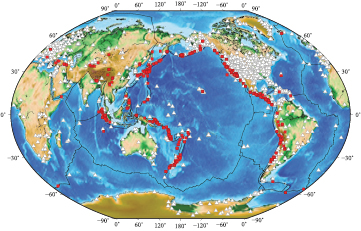
Figure 1. Thousands of continuous GPS stations (white triangles) established for global and regional geodetic applications, earthquakes greater than magnitude 5 (brown squares) since 1990, and major tectonic plate boundaries (black lines). The map is centered on the Pacific Rim, which along with the Indonesian archipelago contains the world's major subduction zones, and has produced nine of the largest ten earthquakes in recorded history.
Download figure:
Standard image High-resolution imageRegional-scale networks, as a natural extension and densification of the global network, now provide coverage of most plate boundaries, primarily by permanent and continuously operating reference stations, referred to as continuous GPS (cGPS) (figure 2). In the early 1990s the first cGPS networks were established in southern California (Bock et al 1997) and the concept quickly spread to other plate boundary zones, and to continental interiors to support surveying and transportation (e.g. Snay and Soler 2008). In this mode, GPS instruments are deployed in secure fixed facilities with a source of power and a communications link to a central facility, and operated autonomously (figure 2). The costs to install a station are significant, but once established maintenance is cost-effective. Initially, cGPS networks recorded data at a 15–30 s interval and data were downloaded to a central facility several times a day to once a day. In the last decade with improvements in data communications and computing power, many stations operate in real time; data are sampled at 1–10 Hz and continuously transmitted to users and to central facilities with a latency of about 1 s. As an example of a robust national network, there are about 1200 real-time stations operating in Japan for monitoring crustal deformation and to support land surveying (Sagiya et al 2000). More than 650 real-time stations are operating for crustal deformation studies and natural hazards mitigation in the Western US and Canada.
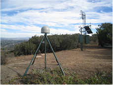
Figure 2. Monument and antenna (under the dome) of a typical cGPS station for monitoring tectonic plate boundary deformation (section 4) and atmospheric water vapor (section 6.1.3), in La Jolla, California. The small white box on the vertical leg contains a MEMS accelerometer used for seismogeodesy (section 5.2.3). See also figure 7 for a schematic of the monument. In the background are GPS equipment enclosures, solar panels, radio antenna for real-time transmission of data, and meteorological instruments. Photo courtesy of D Glen Offield.
Download figure:
Standard image High-resolution imageA cost effective means of further densification is episodic or 'survey-mode' measurements, referred to as sGPS. Prior to the existence of extensive regional networks, this mode was used almost exclusively in GPS geodesy. These surveys can be as accurate as cGPS over the long term if carefully executed, and short-term noise is reduced through multiday occupations. They provide more flexibility than cGPS in establishing inexpensive monuments (e.g. on bedrock), and are particularly useful for local geologic fault crossing surveys or for repeated long-term measurements in remote locations where permanent installations are impractical. GPS surveys have also been conducted in the epicentral regions of large earthquakes in rapid response to seismic events to record coseismic (section 4.7) and postseismic (section 4.6) deformation. However, sGPS is often logistically complex and manpower intensive; it requires teams of surveyors to repeatedly visit and occupy monuments and careful execution in order to replicate to the greatest extent possible the procedures and types of equipment used during each survey. Furthermore, it is of limited use for deriving appropriate noise models for GPS analysis (section 3.3) and for recording transient deformation (section 4.8), but can add information in both cases if the survey points are near cGPS stations, and if deployed expeditiously after a seismic or volcanic event. An intermediate approach involves semi-continuous measurements where instruments operate from 1–3 months at a sub-network of stations and are then moved within a network maintaining some station overlap until the full network is surveyed (Bevis et al 1997, Blewitt et al 2009a, Beavan et al 2010). This process is then repeated to measure station displacements.
2.3. Physical models and analysis
2.3.1. Observables.
GPS geodesy exploits the signal carrier waves to record 'carrier beat phase' observations at both L1 and L2 frequencies, which in simple terms result from the correlation of the signal observed by the receiver with its replica generated by the receiver. The unmodulated carrier wave on either the L1 or L2 frequency can be expressed as

where  is the carrier phase,
  o is the unknown initial phase,
  is the amplitude,
  is the angular frequency, and
  is the wave number. By definition, the signal has phase velocity
with frequency  , wavelength
  , index of refraction n, and the speed of light in a vacuum c. The signal on each frequency is modulated by the various codes including the P-code, C/A code (presently only on L1 and L2C, for the newest satellites), and the satellite navigation message ('the broadcast ephemeris'). The group velocity and phase velocity are related by
Since  and
and  for refraction through the ionosphere and troposphere, the group velocity is always less than the phase velocity, except in propagation through a vacuum, where
  and
and  . It follows that the pseudorange measurements are delayed, while the carrier phase measurements are advanced.
The GPS carrier phase and pseudorange observations are essentially the radio signal time of travel at multiple frequencies from a particular satellite to receiver. The phase measurements are inherently more precise than their corresponding pseudorange measurements because of their effective wavelengths. Considering that the phase and pseudorange measurements with a geodetic GPS instrument can be made with a precision of about 1% of their wavelengths, this translates into 0.002 m in distance for phase compared to 0.3 m and 3 m for P-code and C/A code, respectively. However, the total number of full carrier wave cycles travelled by the GPS signal is unknown and is referred to as the integer-cycle phase ambiguity. The GPS carrier beat phase observations that result from the receiver cross correlation are a fraction of a cycle, or modulo  of the total number of cycles travelled from satellite to receiver. It is beneficial to estimate the number of integer cycles in order to achieve the highest geodetic precision, especially for real-time applications. The pseudorange measurements, although much less precise than the phase measurements, provide valuable constraints on the process of integer-cycle phase ambiguity resolution (section 2.4), and hence on the overall precision of GPS geodesy.
The basic elements of precise GPS positioning can be summarized as a quartet of idealized equations for the phase observations ( ), in distance units, and pseudorange observations (
 ) at frequencies
  and
and  by
by
where  (5) denotes the non-dispersive signal travel distance (the 'geometric term'),
  is the (dispersive) ionospheric effect, and
  and
and  are the integer-cycle phase ambiguities. The objective is to estimate the station position (embedded in
  ), while fixing the ambiguities to their integer values in the presence of ionospheric refraction (section 2.4). In reality, as discussed in the next two sections, the direct GPS signals from satellite antenna to receiver antenna are also perturbed by the non-dispersive neutral atmosphere (the troposphere) and are interfered with by indirect signals (multipath), for example, reflections off objects nearby the GPS antenna. Furthermore, the signal is perturbed by imperfect receiver and satellite clocks, introducing timing and 'clock' biases. Of course, the measurements themselves are subject to error due, for example, to thermal noise in the GPS receiver; errors can vary from one type of GPS receiver to the other. A physical and stochastic model used to invert the observations for the parameters of interest (e.g. position) is discussed in section 2.3.3. Other factors to be considered are phase wind up due to the electromagnetic nature of circularly polarized waves (Wu et al 1993), realizations of reference systems (section 2.5), Earth tides (section 2.5.1), and relativistic effects (section 2.5.5). First, we consider the precise definition of the point to be positioned, antenna phase centers, and metadata.
2.3.2. Phase centers, geodetic marks, and metadata.
To achieve mm-level geodetic precision it is necessary to clearly identify the phase centers of the transmitting satellite antenna (Zhu et al 2003) and receiving ground antenna (Mader 1999), and the exact point ('geodetic mark', 'survey marker') to be positioned. Phase center variations are typically calibrated and applied as known corrections in GPS analysis. There are two types of calibrations for ground antennas. Relative calibrations are derived from GPS observations between two antennas separated by tens of meters at locations with precisely known coordinates and relatively benign multipath environments, with one type of antenna used as the master for calibrations of other types of antenna. Absolute calibrations are derived from a single robot-mounted GPS antenna collecting thousands of observations at different orientations, or by observations within an anechoic chamber (Rothacher 2001). The global GPS community, through the IGS, maintains absolute phase center correction values for all known geodetic antennas, with and without antenna covers ('radomes') (figure 2), at both L1 and L2 frequencies, and for transmitting antennas of different types of satellites (e.g. GPS Block II or GLONASS-M). For ground antennas, the corrections include offsets (in the north, east, and up directions) relative to a particular antenna's reference (mounting) point and variations (<10 mm) as a function of satellite elevation angle and azimuth in 5° increments. In practice, the corrections are imperfect and changes in antenna types will often result in spurious offsets in position. Therefore, changes in antenna type are avoided whenever possible at cGPS stations as well as during repeated field surveys (it is most important in the latter since it is easier to correct for spurious offsets in continuous position time series, see section 3.2). Antennas for cGPS and sGPS are oriented to true north to reduce azimuthal effects and to be consistent with the calibration corrections.
Geodetic applications require a precise definition of the point to be positioned and its relationship to the antenna's phase center. This is typically given as the vertical antenna 'height' although there may be horizontal offsets, as well. The antenna height could be zero if the point is defined at the antenna reference point with respect to which the antenna was calibrated, a small non-zero value if the point is referred to a physical location on an antenna adapter (e.g. 0.0083 m for an adapter specially designed and used in many cGPS networks), or it could be on the order of 1–2 m if the point is defined as a small indentation in a geodetic marker on the ground ('monument'), over which a surveyor's tripod may be mounted. In any case, there are three steps involved in mounting a GPS antenna: Mechanical connection, level, and alignment. The GPS antenna mount needs to be level with respect to the direction of the local gravity field and centered (for example, with a plumb bob) over the mark. Typically, for a cGPS station intended for monitoring crustal deformation, a permanent and rigid monument is constructed (figure 2, see also figure 7) that is isolated from the surface and driven to depth or anchored to bedrock to reduce local surface deformations due to soil contraction, desiccation, or weathering (Williams et al 2004, Beavan 2005), but less expensive spikes mounts, rock pins, masts, building mounts, concrete pillars, etc are also used. The differences and advantages of differing anchoring methods (figure 7) are discussed in section 3.3 in terms of noise characteristics. As an antenna support, cGPS-type anchored monuments have the advantage of being less vulnerable to disturbance. For sGPS, a surveyor's wooden or metal tripod is often used as a base for the antenna, but so are spike mounts and masts. If a surveyor's tribrach (a device for leveling and centering that sits atop a tripod and on which the antenna is mounted) is used, it needs laboratory calibration so as not to introduce a bias into the station position. Alternatively, a rotating optical plummet can be used effectively without calibration. Masts and spike mounts require essentially no calibration. Higher mounted antennas such as a surveyor's tripod or a mast have an advantage over a spike mount in avoiding low elevation-angle obstructions and being less susceptible to low-frequency multipath. A spike mount is less susceptible to operator setup error than a movable tripod or mast and can be left unattended without being seen, a safety issue that can increase survey productivity.
It is critical, in order to achieve the mm-level position precision required by GPS geodesy, to properly record and archive the appropriate 'metadata' for a cGPS or sGPS deployment. At a minimum, metadata include antenna type and serial number, receiver type, serial number and firmware version, antenna eccentricities (height and any horizontal offsets), antenna phase calibration values, and dates when changes in any of these have occurred. Under the global framework of the IGS, keeping the metadata up to date is the responsibility of the Global Archive Centers.
2.3.3. Physical models and observation equations.
Now we present basic functional and stochastic models ('observation equations') that relate the GPS observables and the physical parameters of interest, for example station position, followed by an inversion of the observation equations to estimate the parameters. We assume that the satellite and receiver antenna phase centers and geodetic mark have been well defined and that the metadata are accurate.
GPS signal propagation in a vacuum ('the geometric term') is given by

a non-linear function of the satellite position vector  at the time of signal transmission
  and the receiver position vector
  at the time of reception
  . The receiver position is defined in a right-handed Earth-fixed, Earth-centered terrestrial reference frame (section 2.5.3) by
By convention, the X- and Y-axes are in the Earth's equatorial plane with X in the direction of the point of zero longitude and the Z-axis in the direction of the Earth's pole of rotation (see section 2.5.3 for a more precise definition and figure 3). The satellite position at any epoch of time is described, in state vector representation, by the satellite's equations of motion in a geocentric inertial (celestial) reference frame (section 2.5.2) as
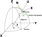
Figure 3. Geodetic coordinate systems. Analysis of GPS phase and pseudorange data is carried out in a global Earth-centered Earth-fixed reference frame in (X, Y, Z) coordinates (6). An alternate representation is geodetic latitude, longitude, and height (ϕ, λ, h) with respect to a geocentric oblate ellipsoid of revolution (one octant shown). Transformation of positions in the right-handed (X, Y, Z) frame to displacements in a left-handed local frame (N, E, U) is a function of geodetic latitude and longitude (36).
Download figure:
Standard image High-resolution imageThe station position in a terrestrial reference frame and the satellite position in an inertial frame are related through a series of rotations (section 2.5.4); in most GPS software the calculations are performed in an inertial frame. The first term on the right of (8) is the spherical part of the Earth's gravitational field. The second term represents perturbing forces (accelerations) acting on the satellite, including the non-spherical part of the Earth's gravitational field, luni-solar gravitational effects, solar radiation pressure, and other perturbations specific to the GPS satellites such as satellite maneuvers. Solving the equations of motion for each GPS satellite based on observations from a global network of GPS stations, referred to as 'orbit determination', provides estimates of the satellite's state ('the satellite ephemeris') at any epoch of time (Beutler et al 1998). Access to accurate satellite ephemerides (at the 1–2 cm level in an instantaneous satellite position) is essential in geophysical applications where the goal is mm-level positioning; the broadcast ephemeris transmitted by the GPS satellites has meter-level precision, not sufficient for most geodetic applications. However, for regional networks (hundreds of km) 5–10 cm errors in individual satellites can still produce mm-level relative coordinates. Precise ephemerides for GPS (and GLONASS) satellites are available through the IGS and are sufficiently accurate for any geodetic application. Although of intrinsic interest as an orbit determination problem for large irregular satellites occasionally subject to maneuvers and the complex modeling required for solar radiation pressure effects, for most physical applications and for simplicity we will assume that the GPS ephemerides are given and without error (not estimated in the inversion process).
We can express the GPS inverse problem starting with a general non-linear functional model  , where the physical parameters of interest
  are estimated from GPS phase and pseudorange observations contained in vector
  . The model for an L1 or L2 phase measurement
  at a particular epoch of time can be expressed in distance units by the observation equation
where  (5) denotes the geometric (in vacuum) distance between station i and satellite j, t is the time of signal reception,
  is time delay between transmission and reception, and c is the speed of light. The second term on the right includes dti the receiver clock error and
  is the satellite clock error; for our purposes we will simply refer to it as the clock error dt.
  is the tropospheric propagation delay in the zenith direction ('zenith total delay') and
  is a function that maps the ZTD to lower elevation angles (see section 6.1.2 for additional horizontal troposphere delay gradient parameters).
  is the total effect of the ionosphere along the signal's path (section 6.2.1).
  denotes the integer-cycle phase ambiguity, Bi and Bj denote the non-integer (fractional) parts of receiver- and satellite-specific clock biases, respectively, and
  is the wavelength at either the L1 or L2 frequency. The term
  denotes total signal multipath effects at the transmitting and receiving antennas; for our purposes we will neglect multipath at the satellite transmission antenna and refer to this term as
  . Finally,
  denotes measurement error, whose assumed first- and second-order moments are described below after linearization of the observations equations.
The observation equation for a P1 or P2 pseudorange measurement is the same as the phase (9) except that there is no ambiguity term  and the sign is reversed for the dispersive ionosphere term
  . As mentioned previously, the uncertainties in the longer wavelength pseudorange measurements are about two orders of magnitude larger than for the phase errors. At each observation epoch, the number of observations is four times (L1, L2, P1, P2) the number of visible satellites. The number of estimated parameters depends on the application and the parameters of interest.
The integer cycles are counted once tracking starts to a satellite so only the initial integer-cycle phase ambiguities  need to be estimated. However, in practice phase observations may include losses of receiver phase lock and cycle slips (jumps of integer cycles) due to a variety of factors including signal obstructions, severe multipath, gaps in the data due to communication failures, satellite rising and setting, severe ionospheric disturbances, etc. One outcome is losing count of the number of integer cycles in the signal propagation, which complicates phase ambiguity resolution (section 2.4) and reduces the precision of the parameters of interest, if not taken into account. Therefore, efficient geodetic GPS algorithms need to include automatic detection and repair of cycle slips and to account for gaps in the phase data.
Neglecting second-order ionospheric effects (Kedar et al 2003), the 'ionosphere-free' linear combination of the L1 and L2 phase observables (in units of phase) is given by
so that the non-integer ambiguity term for  is
is

The variance in the ionosphere-free combination is by error propagation
assuming that the L1 and L2 variances,  and
and  are of equal weight (=
 and uncorrelated. In most cases (except for very short baselines in network positioning described below), phase observations
  and
and  are combined to form
  since the increase in variance is negligible compared to the differential ionospheric signal delay.
Depending on the application, 3D positions (6), zenith troposphere delays  , ionospheric delays
  , and multipath effects
  (9) may be parameters of specific physical interest ('signals'). For example, the ionospheric parameters
  may be eliminated to first order through the linear combination of phase measurements (10), but are of interest in tsunami modeling based on gravity wave and acoustic wave disruptions of the ionosphere (section 6.2). Similarly, the troposphere parameter is of interest in short-term weather forecasting (section 6.1.3) and climate change research (section 7.5). Thermal receiver noise and multipath effects are considered to be random 'noise' in the context of a precise GPS, although receiver multipath
  can also be exploited as a 'signal' for environmental applications (section 8.5). The term
  and the clock error term are considered 'nuisance' parameters.
The model equations  are linearized through a Taylor series expansion

that can be expressed as
Since phase and pseudorange observations are subjected to some error  , the observation equations with assumed first-order (mean) and second-order moments (variance) can be expressed as

A is called the design matrix of partial derivatives, E denotes statistical expectation, D denotes statistical dispersion,  is a covariance matrix of observation errors, P is the weight matrix, and
  is an a priori variance factor. If we assume that the observations are uncorrelated in space and time, the covariance matrix
  is diagonal. Linearization of the observation equation (9), here for the ionosphere-free linear combination (LC), for a particular station i and satellite j at any epoch of observation is

The  symbol denotes incremental adjustment to an estimated parameter relative to its a priori value in the linearization of observation equations (9). For example,
  is the partial derivative for the position parameters such that
where  and
and  are the station and satellite positions, respectively. The subscript LC for the error term
  denotes that the error refers to the ionosphere-free observable (12). Note that multipath is dispersive (and correlated in time) (section 8.4) and
  denotes the magnified effect.
Here we describe a weighted least squares (used several times in this review) for the inversion of (15) whereby the Euclidian norm (L2-norm) of the residual vector  is minimized such that

with the weighted least squares solution  and the estimated covariance matrix
  given, respectively, by
The hat denotes an estimated quantity. The vector  contains the post-fit residuals. The a posteriori variance factor
  is often called the 'a posteriori variance of unit weight', 'chi-squared per degrees of freedom', or 'goodness of fit', where the degrees of freedom is
  ;
;  is the number of observations and
  the number of parameters. In most cases, there is some a priori value for a subset of the parameters in vector
  (e.g. the position), which can be introduced into the above model with its diagonal covariance matrix
  such that

2.4. Positioning approaches
There are two basic approaches to GPS analysis. The earliest one is network ('relative') positioning (Dong and Bock 1989, Blewitt 1989) developed to position stations with respect to at least one fixed reference station within a local or regional network. Network positioning is also used to estimate satellite orbits and Earth orientation parameters (EOP) from a global network of reference stations. With the significant increase in the number of networks and the number of stations within networks, relative positioning became computationally cumbersome. Precise point positioning (PPP) (Zumberge et al 1997) was introduced as a way to individually and very efficiently estimate local and regional station positions directly with respect to a global reference network, the same one used to estimate the satellite orbits. The longest lived and most widely used software packages for precise GPS positioning and orbit determination covering both approaches include Bernese (at the Astronomical Institute, University of Berne: Beutler et al 2001, Hugentobler et al 2005), GAMIT ('GPS at MIT', Herring et al 2008), and GIPSY-OASIS ('GNSS-Inferred Positioning System and Orbit Analysis Simulation Program' at NASA's Jet Propulsion Laboratory: Zumberge et al 1997, Bertiger et al 2010). Other packages include NAPEOS ('NAvigation Package for Earth Orbiting Satellites, European Space Agency: Springer, 2009), PAGES ('Program for the Adjustment of GPS Ephemerides' at the US National Geodetic Survey: Eckl et al 2001), PANDA ('Position and Navigation Data Analyst' at Wuhan University: Liu and Ge 2003), and EPOS ('Earth Parameter and Orbit Software' at GeoForschungsZentrum, Potsdam: Angermann et al 1997). GPS analysis by these and other software has evolved with improved physical models and processing efficiencies, and has significantly benefited by the expansion of the global network under the aegis of the IGS (section 2.2), providing increasingly accurate GNSS orbit estimates (currently GPS and GLONASS) and more stable reference frames.
The simplest network for network positioning consists of two stations, a 'baseline vector' in geodetic parlance, one with fixed coordinates and one with an unknown position. In practice, networks at local to regional scales may consist of hundreds of stations, e.g. a network designed to span a tectonic plate boundary. In this method, the observation equations (9) for the two stations that determine the baseline are differenced so that the unknown parameters are the baseline vector components, not the absolute positions. In precise point positioning (PPP), an unknown station is directly positioned with respect to the same terrestrial frame, but now realized through known precise satellite ephemerides and satellite clock estimates estimated from the same global tracking network that defines the reference frame (Kouba and Heroux 2001). Network positioning and point positioning approaches can be considered equivalent in terms of the underlying physics. In both methods, positions are estimated with respect to the International Terrestrial Reference Frame, the latest version being ITRF2008 (section 2.5.3) (Altamimi et al 2011). The main advantage of PPP is the speed of computations in the inversion process (18) and (19). The efficiency of network positioning decreases with the number of stations (approximately as the cube of the number of stations), and becomes unwieldy as the number of stations grows. One approach to improve its efficiency is to divide the larger network into subnetworks with overlapping stations and then combine the subnetworks through a least squares network adjustment (Zhang 1996) or even to analyze the larger network baseline by baseline, in which case PPP and network positioning are nearly equivalent in terms of computational time. To improve accuracy it is useful to resolve integer-cycle phase ambiguities  (9) to their correct integer values (Counselman and Gourevitch 1981, Blewitt 1989, Dong and Bock 1989, Teunissen 1998 and references therein). The original PPP formulation did not include ambiguity resolution, while ambiguity resolution was always part of the network positioning approach. In section 2.4.2, we present a way to resolve phase ambiguities within PPP analysis at regional scales (up to about 4000 km).
2.4.1. Network positioning.
In network positioning 'common-mode' errors are cancelled by differencing the phases collected between stations so that the satellite clock biases  terms drop out since they are common to both stations, and by differencing between satellites so that the station clock biases
  terms drop out since they are common to both satellites, thereby revealing the integer-cycle phase ambiguities
  . This 'double differencing' is performed at each observation epoch for all stations in a network of receiving stations and all visible satellites. Estimating the satellite and receiver clock biases on an epoch by epoch basis is, assuming that the clock biases are uncorrelated in time, equivalent to double differencing (Schaffrin and Grafarend 1986). Likewise, 'common-mode' errors due to tropospheric and ionospheric refraction are reduced. At the very shortest distances (up to several kilometers), the satellite/receiver paths sample the same portion of the atmosphere and, thus, atmospheric effects are very similar and often assumed identical. This assumption degrades as the distance between stations increases. For the troposphere (section 6.1), the correlation length is on the order of tens of kilometers; for the ionosphere (section 6.2) the effect is approximately proportional to the distance. It should be noted that for short distances (<2–3 km) the increase in noise level when forming the ionosphere-free combination (10) is greater than the reduction in the ionospheric effect
  , and so the L1 and L2 observations can be directly inverted. In this case, rapid ambiguity resolution is robust even with a single epoch of L1 observations (e.g. instantaneous positioning, Bock et al 2000). This type of solution is useful, for example, for near geologic fault crossing arrays of GPS stations to quantify the degree of fault coupling (creep—section 4.5). However, these are special cases and for most applications ionosphere-free observables are used in the inversion (16) for the parameters of interest.
Although it is possible to eliminate first-order dispersive ionospheric effects  (9) by (10), in fact it is the ionosphere that is the primary limitation to successful ambiguity resolution. This is because the phase ambiguity term resulting from the ionosphere-free linear combination has a non-integer value (10). One solution is to use the pseudorange observables to extract the integer-cycle phase ambiguities
  and
and  by first estimating
  , the so-called 'wide-lane' or 'Melbourne–Wübbena' combination with an effective wavelength of 86.2 cm, compared to the narrower wavelength L1 (~19 cm) and L2 (~24 cm) phase observations (Hatch 1991, Melbourne 1985, Wübbena 1985), where

Once the  ambiguities are resolved then one can try to resolve the 'narrow lane'
  ambiguities (now with an effective wavelength of 10.7 cm). Usually, the wide lane ambiguity can be resolved, even for networks of global extent, by inverting multiple data epochs at static stations, as long as the pseudorange errors are a fraction of the wide-lane wavelength, as is the case for modern GPS receivers. This is more complicated for real-time (single epoch) observations and dynamic platforms. The main sources of error are the magnitude of the dispersive ionospheric refraction and receiver multipath effects, which are magnified in the ionosphere-free combination. Another approach to resolving the wide-lane ambiguities, appropriate to network positioning, is to apply a realistic a priori stochastic constraint (a 'pseudo' observation) on the ionosphere term
  as a function of the inter-station distance (Schaffrin and Bock 1988).
Intrinsic to ambiguity resolution is examining the estimated real-valued doubly-differenced integer-cycle ambiguities and picking out the corresponding correct integer values through some deterministic or stochastic criteria. The simplest approach is to round the real-valued ambiguity to its closest integer value if the uncertainty in the real value is within a certain tolerance (e.g. 0.1 of a cycle). Another approach is to attempt to resolve ambiguities in sequence of increasing baseline length, under the assumption that shorter baselines are subject to fewer errors due to orbital error and atmospheric refraction (Abbot and Counselman 1989, Dong and Bock 1989). However, this approach was suggested when orbital error dominated the GPS analysis error budget. In current practice with the availability of IGS orbits, local conditions (multipath, atmospheric refraction) are dominant up to ~1000 km, where shorter periods of mutual visibility are the issue. An efficient approach is the 'least-squares ambiguity decorrelation adjustment' (LAMBDA) method (Teunissen 1995). It first decorrelates the doubly-differenced phase ambiguities based on an integer approximation of the conditional least-squares transformation that reduces the ambiguity search space bounding all possible integer candidates. This is a multi-dimensional problem according to the number of ambiguities; in three dimensions the transformation can be viewed as changing a very elongated ellipsoidal search space into one that is more spheroidal. However, decorrelation is never complete. Consider that  is the ambiguity transformation and operates on the portion of the design matrix A (13) that corresponds to the vector a of real-valued ambiguities, and that the remainder of A contains all the other parameters (e.g. station positions). Then

and the equivalent minimization problem becomes

The search space is then
where  is a user-defined constant and
  is the variance, where the vertical line denotes 'given'. The ambiguities are then resolved according to the sequential bounds of the transformed ambiguity space, starting with the transformed ambiguities of lowest uncertainty. Once the ambiguities are resolved to integers, they can be used to estimate the remaining parameters of interest (Teunissen 1998). The above transformed ambiguity approach can be applied to the L1, L2, or wide-lane ambiguities (22), and the process could be supplemented by taking into account the properly weighted pseudorange measurements. In the most general case, the search space of dimension of the number of, say, wide-lane ambiguities, is given by
where  is the user-defined threshold,
  is the determinant of the portion of the normal matrix
  (19) containing the phase ambiguities,
  and
and  are the carrier-phase and pseudorange uncertainties, respectively, n is the number of epochs, and
  and
and  are the L1 and L2 carrier-phase wavelengths. This shows that for static GPS solutions, the integer ambiguity resolution should improve with the number of observation epochs and the wavelength, which is longer (~86 cm) for the wide-lane ambiguities (Geng and Bock 2013).
2.4.2. Precise point positioning.
Precise point positioning (PPP) (Zumberge et al 1997) relies on pre-computed true-of-observation-time satellite positions  (5) and satellite clock parameters
  (9) estimated through a network analysis of globally-distributed reference stations, as is done and distributed by the IGS and its analysis centers (Kouba and Heroux 2001). These are the same IGS stations whose ITRF coordinates and velocities are used to realize the international terrestrial reference system (section 2.5.1), and so their 'true-of-date coordinates' at a particular epoch of time are known with mm-level accuracy. As its name implies, PPP calculates 'absolute' positions at any location on the globe with respect to the ITRF (section 2.5.3), which is accessible through the given satellite orbit and clock parameters. The parameters estimated in the PPP inversion are then the station's position, zenith troposphere delays
  at that location (i = 1), the receiver clock parameter
  , and the non-integer bias term
  for each satellite j (9). The ionosphere parameters
  are eliminated to first order by linear combination of the L1 and L2 phase observations (10). It is important that the physical models (e.g. Earth tides, antenna phase center corrections) used in the PPP inversion be the same as those used in the global network analysis. This is accomplished through standards adopted by the IGS.
In order to extend the PPP method to allow for ambiguity resolution (AR) (PPP-AR, Ge et al 2008, Laurichesse et al 2009, Geng et al 2012) within a limited area of interest (up to a scale of about 4000 km), another network solution is performed. This solution estimates the weighted averages of all  satellite bias terms (9), called fractional cycle biases (FCBs), so that these parameters can also be fixed, prior to the site-by-site PPP-AR position calculations within the area of interest. The reference stations for this network solution are chosen to be outside the region of interest so that, for example, coseismic motions will not affect FCB parameter estimation, an approach that is especially suited for real-time earthquake monitoring (section 5.2). After resolving the wide lane ambiguities
  (22) as part of the network solution, the linearized narrow-lane ionosphere-free carrier phase observation equations for a particular station i and satellite j at each epoch of observation are
where now  denotes the narrow lane ambiguity, with
  (Geng et al 2013). The
  symbol denotes incremental adjustment to an estimated parameter relative to its a priori value in the linearization of observation equations (9).
  is the partial derivative for the position parameter (17). The subscript LC for error
  , such that
  , denotes that the error refers to the ionosphere-free linear combination. In the inversion of (27) the estimated parameters
  are real-valued. Again, we have assumed that the precise satellite orbits
  and satellite clock parameters are available from the IGS, or another external source, and held fixed. The station coordinates are also held fixed in the network solution to their true-of-date values with respect to the ITRF, derived from time series analyses of years of daily positions (section 3.2); alternatively, the stations themselves may be IGS reference stations so their true-of-date coordinates are known by convention (e.g. ITRF2008). The receiver bias
  is eliminated by differencing the observation equations (27) between satellites. In the inversion, the fractional part of
  ,
,  is estimated for each station in the reference network as well as the zenith troposphere delays
  , the clock parameter
  , and the narrow-lane ambiguities. A mean value for the satellite phase bias
  for each satellite j, called a fractional cycle bias (FCB), is then estimated over the r reference stations by
Increasing the number of stations in the reference network will improve the reliability and accuracy of the FCB estimates.
We can now individually perform PPP-AR inversions for each unknown station position in the area of focus using, importantly, the same model (27) and inputs as the prior network inversion. As before, we hold fixed the precise satellite orbits  and satellite clock parameters obtained from the IGS, and the receiver bias
  is eliminated by differencing between satellites. The satellite bias
  for each satellite is assigned the FCB value
  . As a result, the integer-valued phase ambiguities
  (27) have been decoupled from the satellite and receiver phase biases. Ambiguity resolution for a single station can then be attempted. Upon successful fixing (or partial fixing) of
  to integers, e.g. using the LAMBDA method, the precise point positioning with ambiguity resolution (PPP-AR) solution for an individual station (client) is achieved, and the estimated coordinates are 'absolute' with respect to the ITRF (section 2.5.3). The point positioning method is particularly advantageous, compared with network positioning, for the case of estimating coseismic motions (section 5.2). Regional network positions may be contaminated when all stations are displaced during an earthquake. In the case of great earthquakes, since the zone of coseismic deformation may extend to distances of thousands of kilometers from the earthquake's epicenter, the solution that provides the FCB corrections may be biased. One could then revert to PPP without ambiguity resolution and take advantage of any collocated strong motion accelerometer data (next section) to improve the precision of the coseismic station displacements.
Up to this point we have assumed that the inversion of GPS data (15) and (25) for parameters of interest is performed using a linearized weighted least squares algorithm (19). In practice, the inversion is often extended to a weighted least-squares algorithm, where realistic uncertainties are assigned to a priori estimates of particular parameters (15), e.g. station positions and satellite orbital elements may be tightly constrained in GPS meteorology (section 6.1.3). Kalman filters or similar formulations may be used to take into account temporal correlations in the estimated parameters. In the above PPP-AR example, troposphere delays and receiver clock parameters may be parameterized by piecewise continuous functions with assumed stochastic processes, e.g. first order Gauss–Markov (46), to account for temporal correlations in the phase and pseudorange observables.
2.4.3. Addition of accelerometer observations.
Precise GPS measurements are often supplemented with data from other sensors, e.g. accelerometers for monitoring of seismic displacements and velocities (section 5.2.3), or inertial navigation units for precise trajectories for airborne lidar measurements of active fault zones (Nissen et al 2012, Brooks et al 2013). Here we present a supplement to the GPS observation equations (27) for the addition of accelerometer observations, suitable for the inversion of positions and velocities with a Kalman filter discussed in detail in section 5.2.3. We modify the linearized observation equations (27) to explicitly introduce notation for time epoch k

The notation i here is somewhat redundant since there is only one station to position; it is used to denote station dependence. In addition to the positions  , the parameter set includes seismic velocities
  . The linear accelerometer observation equation (31), one for each accelerometer channel (local north, east, and up), includes
  the observed accelerometer measurements,
  true accelerations,
  the acceleration biases, and
  the accelerometer random error such that
  . The biases
  can be estimated as a stochastic process to accommodate slowly time-varying changes. Hence, no pre-event mean needs to be eliminated from the acceleration data before starting the Kalman filter. Accelerometer errors due to instrument rotation and tilt ('baseline' errors in seismology parlance) that are manifested in doubly-integrating accelerations to displacements (section 5.2.2) are minimized since these biases are absorbed by
  . The state transition matrix for the Kalman filter takes the form of

where  is the sampling interval of the accelerometer data. The accelerometer data are applied as tight constraints on the position variation between observation epochs when, as is usually the case, the sampling interval of accelerometers in 100–250 Hz but only 1–10 Hz for GPS. This approach is suitable for a 'tightly-coupled' Kalman filter inversion since it combines the accelerometer and GPS data at the observation level (Geng et al 2013, Yi et al 2013). It is distinguished from a 'loosely-coupled' Kalman filter, where the accelerometer measurements are included after a station displacement estimate has been achieved, either through PPP or network positioning (Bock et al 2011). The tightly-coupled approach is expected to improve cycle-slip repair (section 2.3.3) for GPS carrier-phase data and rapid ambiguity resolution after GPS outages (Grejner-Brzezinska et al 1998, Lee et al 2005, Geng et al 2013a).
2.5. Reference systems for space geodesy
2.5.1. Overview.
A GPS measurement is the time of travel of a signal from the satellite's transmission to its reception on the ground; in that interval of time (~0.07 s) the apparent position of the station has changed by about 3 m due to the Earth's rotation. Positioning requires, therefore, a well-defined celestial (inertial) reference system in which to describe the satellite's motion (section 2.5.2), a terrestrial reference system that is fixed to the solid Earth and rotating with it (section 2.5.3), transformation parameters between two systems (section 2.5.4), and precise time measurement within the space-time framework of General and Special Relativity (section 2.5.5). The celestial reference system defined for the GPS and other near-Earth satellites, as described in this section, is the Geocentric Celestial Reference System (GCRS); the terrestrial reference frame is the International Terrestrial Reference System (ITRS).
Geodesy as the study of the Earth's size, shape, and deformations has always involved point observations of extraterrestrial bodies along with distance and angle measurements between points on the Earth's surface. The first observations of the size of the Earth by Eratosthenes used geometry, Sun observations, and distances travelled by camel caravans (Wilford 1981). Terrestrial measurements of angles (triangulation) and distances (trilateration), astronomical observations to the Sun and stars (geodetic astronomy), and improved timekeeping were used to establish orientation (azimuth) with respect to true north and an observer's origin (astronomical latitude and longitude of terrestrial stations) (Mueller 1969).
Astronomical observations revealed motion of the Earth's pole of rotation with respect to the pole of the ecliptic (the apparent path of the Sun's motion on the celestial sphere as seen from Earth) due to the gravitational potential of the Moon, the Sun, and the planets acting on the Earth's equatorial bulge, and the Earth's gravitational potential perturbed by the external tidal potential. These motions with different periods are called precession and nutation. Precession includes the sum of two effects, luni-solar and planetary precession. Luni-solar precession is the slow circular motion of the celestial pole with a period of ~25 800 years, with an amplitude equal to the obliquity of the ecliptic, about 23.5°, resulting in a westerly motion of the equinox on the equator of about 50.3'' per year. Planetary precession consists of a slow 0.5° per year rotation of the ecliptic about a slowly moving axis of rotation resulting in an easterly motion of the equinox by 12.5'' per century and a decrease in the obliquity of the ecliptic by 47'' per century. Nutation is the relatively short-period motion of the Earth's pole of rotation, superimposed on the precession with oscillations of one day to 18.6 years (the main period) and a maximum amplitude of 9.2''. As geodetic astronomic observations became more precise and global in scale, changes in position relative to the Earth's rotation axis became apparent (Munk and MacDonald 1975). The 'Chandler wobble' detected in the late 19th century revealed a change in the Earth's axis of rotation with respect to the solid Earth in a somewhat counterclockwise circular motion with a period of about 433 d and a total magnitude of about 9 m. It represents the 'free' component of polar motion if all external torques on the Earth were removed; the Earth's rotation axis still varies with respect to its figure, primarily due to the Earth's elastic properties and to the exchange of angular momentum between the solid Earth, the oceans (Ponte et al 1998), and the atmosphere. Using data and models over two decades, the Chandler wobble was found to be primarily excited by ocean-bottom pressure fluctuations (Gross et al 2003). The 'forced' component of polar motion due to tidal forces includes an annual component due to atmospheric excitation with a nearly constant amplitude of about 100 mas (milliarcseconds), nearly as large as the Chandler wobble's 100–200 mas, a quasi-periodic decadal component with an amplitude of about 30 mas, a linear trend having a rate of about 3.5 mas yr−1, and nearly diurnal motions of smaller magnitude (Gross 2000).
To facilitate an unambiguous connection between the celestial and terrestrial reference systems, the definition, by international convention, of a Celestial Intermediate Pole (CIP) seeks to separate motions with respect to the GCRS and the motion of the pole in the ITRS into a 'celestial' and 'terrestrial' part (Petit and Luzum 2010). This is complicated by the tidal response of the Earth. Instantaneous locations of points on the Earth's surface are affected in a complex manner by the tidal potential due to the gravitational potential of the Sun and Moon including the solid Earth tides (with a maximum displacement of about one meter, (Melchior 1983, Scherneck 1991), ocean loading (the elastic response of the Earth to mass loading by ocean tides that can reach 100 mm (Farrell 1972, Agnew 2012), atmospheric loading (the elastic response of the Earth to mass loading by atmospheric barometric pressure at the several millimeter level (Van Dam and Wahr 1987, Ray and Ponte 2003), and the response of the Earth's crust to polar motion (the 'pole tide' at the centimeter level (Miller and Wunsch 1973)). It should be noted that GPS positions are also affected by non-tidal atmospheric loading, which has a seasonal effect that is not well modeled (section 3.4).
2.5.2. Celestial reference system.
The advent of radio astronomy in the 1960s began a shift from a celestial reference system tied to a star catalogue to one tied to extragalactic radio sources that better approximate a point in space (less proper motion). Currently, the International Celestial Reference System (ICRS) (Petit and Luzum 2010) defined through resolutions of the International Astronomical Union (IAU) is realized through a Celestial Reference Frame (CRF) defined by a catalogue of positions (right ascensions and declinations on the celestial sphere) of nearly 300 extragalactic radio sources (primarily quasars) observed by very long baseline interferometry (VLBI) radio telescopes (Ma et al 1998), assumed to have no net proper motion. The International Celestial Reference Frame 2 (ICRF2) was released in 2009; the previous definition was released in 1995 and endorsed in 1997 by the IAU. The source positions are known to an accuracy of better than a milliarcsecond, limited by the structure of the sources at the observed radio frequencies. The equatorial plane is defined as the mean equator at time J2000.0 (Julian date 2451545.0 on January 1 at 2000 12 h—section 2.5.5). The motion of the celestial pole (z-axis) is due to precession and nutation. Its position is consistent with catalogs of fundamental stars (e.g. Fifth Fundamental Catalog—FK5) to within about 50 mas. The x-axis of the ICRS, the origin of right ascension, is taken as the dynamical equinox at J2000.0. In theory, the ICRF consisting of a list of celestial coordinates is independent of the definition of a celestial equator, equinox, and ecliptic. However, these concepts continue to be relevant so as to be consistent with astronomical catalogs and earlier reference frames used in space geodesy. The ICRS is a barycentric system defined for describing the motion of objects located outside the gravitational attraction of the Earth. The GCRS, used in the remainder of this review, is a geocentric system defined for near-Earth satellites including GPS, which is consistent with the ICRS and is defined through conventions of the International Astronomical Union (Petit and Luzum 2010).
2.5.3. Terrestrial reference system.
The terrestrial Earth-centered Earth-fixed reference system, the ITRS, is also defined by convention through resolutions of the International Union of Geodesy and Geophysics (IUGG). It is realized through the International Terrestrial Reference Frame (ITRF) defined by a catalogue of the 3D positions (6) and velocities of several hundred space geodetic stations. The velocities are needed to account for tectonic plate motions (section 4). As the number of space geodetic stations and positioning precision have increased, as well as changes in underlying models and refinements in the definition of the ITRS and in processing software, a new ITRF version has been released every few years, starting with ITRF88. The latest incarnation is ITRF2008 (Altamimi 2011), with a new version (ITRF2014) in preparation. ITRF2008 is based on four space geodetic methods: Satellite laser ranging (29 years of data), very long baseline interferometry (26 years), GPS (12.5 years), and DORIS (Doppler Orbitography and Radiopositioning Integrated by Satellite) (16 years), from a total of 934 stations at 580 sites (some sites have multiple geodetic markers). Each method has a corresponding international body that coordinates its activities: International Laser Ranging Service, International VLBI service for Geodesy and Astrometry, International GNSS service, and International DORIS service). Some sites have collocated instruments, with each instrument referred to as a separate 'station' with local survey ties between the different instruments at 91 of the sites (the precision of the local ties is a significant source of error, and is complicated by identifying the reference point for each instrument). The sites are unevenly distributed geographically with about four times the number in the northern hemisphere than in the southern hemisphere. The origin of the reference frame is defined to be at the Earth's geocenter (with translation rates) as derived from satellite laser ranging (SLR) to specially designed satellites that are small, dense, and of spherical shape with well-defined and stable phase centers. The scale is such that there is a zero scale rate compared to the mean scale and scale rate derived from select SLR and VLBI position solutions.
Up to and including ITRF2008, the frame was defined by the coordinates and velocities of global tracking stations, which included secular (steady) plate motions. However, this approach is complicated by coseismic and postseismic deformation (sections 4.6 and 4.7). Large earthquakes can displace large regions and nullify the assumption of a secular change in coordinates at affected stations and distort the reference frame; this is particularly pronounced for very large events such as the 2004 Mw 9.3 Sumatra earthquake. Other complications include station motions that deviate from the secular. Tidal effects are removed, within their uncertainties, through conventional models, and so station coordinates are with respect to a tide-free frame (section 2.5.1). Other motions include intraplate deformation, subsidence that may have both horizontal as well as vertical components, volcanic deformation, etc. Thus, the choice of suitable ITRF reference stations is challenging. A more realistic approach is to define the reference frame through the observed 'trajectory' of the stations through GPS analysis, wherever they may be, on stable plate interiors or plate boundaries (Bevis and Brown 2014). The frame is dynamic in the sense that it changes and is improved as more data are collected. This is an iterative approach, but is more amenable to continuity compared to periodic updates to ITRF, as has been the common practice. According to Altamimi, ITRF2014 will take into account the effects of earthquake-induced deformation by estimating coseismic offsets and postseismic deformation through parametric models (logarithmic or exponential decay). This involves rigorous time series analysis of coordinate time series and is complicated, as is the conventional ITRF approach, by apparent changes in position due to mundane factors such as changes in GPS antenna types and metadata errors, which are manifested as apparent offsets in the coordinate time series (section 3.2).
2.5.4. Celestial/terrestrial system transformations.
The transformation from the Geocentric Celestial Reference System (CGRS) to the International Terrestrial Reference System (ITRS) can be expressed through a series of rotations that, historically, include the effects of nutation, precession, and Earth orientation parameters (EOPs) consisting of nine separate 3D rotations, summarized as (Mueller 1969),

The matrix product NP is a series of six successive rotations including the effects of precession and nutation (section 2.5.1). The matrix S

includes the EOPs (xp, yp, and the Earth Rotation Angle.— ) transformation. The EOPs provide the permanent tie of the GCRS to the ITRS. They describe the orientation of the CIP in the terrestrial system (two polar motion parameters: xp, yp) and in the celestial system (two celestial pole offsets d
 , the nutation in longitude and d
 , the nutation in obliquity, (Mueller,1969)) and the orientation of the Earth around this axis (
 —section 2.5.5), as a function of time. The time derivative of the
  is the Earth's angular velocity. The 3 × 3 rotation matrix
  represents a right-handed rotation about the i axis (i = 1, 2, 3) with a positive rotation when looking toward the origin from the positive axis, e.g.
To avoid ambiguity, 'the celestial motion of the CIP (precession and nutation) includes all terms with periods greater than 2 d in the GCRS, i.e. frequencies between −0.5 cycles per sidereal day (cpsd) and 0.5 cpsd. The terrestrial motion of the CIP (polar motion), includes all terms outside the retrograde diurnal band in the ITRS (i.e. frequencies lower than −1.5 cpsd or greater than −0.5 cpsd)' (Petit and Luzum 2010). The maintenance of the reference systems and their realizations are the responsibility of the International Earth Rotation and Reference Systems Service (IERS).
In GPS analysis, models of these mostly periodic motions and their effects on position are adopted as part of the reference system definitions, and are taken as fixed. Thus, estimated GPS positions are given with respect to a 'conventional tide free crust', where the effects of the permanent tidal potential, which are the cause of semi-diurnal and longer period oscillations of positions on the Earth surface, are modeled; hence, these oscillations are effectively removed since the model predictions are expected to be at least as accurate as the geodetic data (~1 mm level in displacement). However, this is not the case for the EOPs, which are estimated as part of global GPS analysis and by other space geodetic methods, and are made available for positioning through the IGS. Therefore, the accuracy of the transformation between the GCRS and ITRS is effectively dependent on the EOPs, which have an accuracy of about 0.1 mas (~3 mm in displacement at the Earth's surface) in each component. Besides GPS, the main contribution of VLBI to maintaining the reference systems is through the ERA angle and providing the connection to an external celestial reference frame; the main contribution of SLR is a precise location of the Earth's geocenter. Earth orbiting satellites are perturbed by the Earth's and Moon's gravitational potential, the Earth's atmosphere, and the Sun's radiation (solar radiation pressure). Being close to the Earth, satellite motion (orbits, ephemerides) is expressed through six Keplerian elements at any instant in time, or equivalently by an inertial (celestial) state vector comprising 3D positions and velocities (7) and (8) within the quasar-realized celestial reference frame.
2.5.5. Time systems.
In this section we describe the time systems relevant to GPS geodesy and their relationship to civilian time keeping. Two aspects of time are important, the epoch and the interval. The epoch defines the moment of occurrence and the interval is the time elapsed between the two epochs in units of some time scale. Two time systems are in use today, atomic time and dynamical time. The unit of time t in (5) is the independent variable in the equations of motion of bodies in a gravitational field, according to the theory of General Relativity. An Earth-based clock will exhibit periodic variations as large as 1.6 msec with respect to the motion of the Earth in the Sun's gravitational field. For GPS geodesy, it is sufficient to use terrestrial time (TT), which represents a uniform time scale for motion in the Earth's gravitational field, which is related to proper time and other relativistic (barycentric) time scales (Petit and Luzum 2010). The coordinate system generally used when including relativity in near-Earth orbit determination solutions is the GCRS. The accuracy of the GPS clocks is affected by both Special and General Relativity. Because of Special Relativity the satellite atomic clocks fall behind clocks on the ground by about 7 mas per day due to the time dilation effect of their relative motion. On the other hand, due to the curvature of spacetime in General Relativity the satellite clocks will appear to run faster by about 45 mas per day. The next effect of 38 575.008 ns d−1 will result in a position error of about 10 km a day if not taken into account. In GPS analysis a nominal frequency offset and a periodic relativistic correction derived as a dot product of the satellite position and velocity vectors compensate for this effect. Provision must be made for departures in the GPS satellite orbits (in particular in its semi-major axis and its distance from the Earth's mass), which can reach up to 10 ns d−1 in apparent clock rate, and for the Earth's gravity field oblateness (Kouba 2004). Ignoring these effects can result in errors in the relativistic transformation (Petit and Luzum 2010) of 0.2 ns d−1 and periodic errors of 0.1 and 0.2 ns, with periods of about 6 h and 14 d, respectively (Kouba 2004). They impact the accuracy of the GPS orbits calculated by the IGS and need to be taken into account for estimating accurate IGS satellite clock parameters.
Atomic time is the basis of a uniform time scale on the Earth and is realized by International Atomic Time (TAI); for historical reasons there is a constant offset between TT and TAI, i.e. TT = TAI + 32.184s. Prior to the advent of atomic time, the civilian time system was based on the Earth's diurnal rotation and was termed universal time. The TAI epoch of origin was established to coincide with universal time (UT) at midnight on 1 January 1958. At this date, universal time was superseded by atomic time for civilian timekeeping. TAI is a continuous time scale, maintained by the Bureau International des Poids et Mesures (BIPM), using data from about three hundred atomic clocks in over 50 national laboratories. The fundamental interval unit of TAI is one SI second defined at the 13th general conference of the International Committee of Weights and Measures in 1967 as the 'duration of 9 192 631 700 periods of the radiation corresponding to the transition between two hyperfine levels of the ground state of the cesium 133 atom'. The SI day is defined as 86 400 s and the Julian century as 36 525 d. The time epoch denoted by the Julian date (JD) is expressed by a certain number of days and fraction of a day after a fundamental epoch sufficiently in the past to precede the historical record, chosen to be at 12h universal time (UT) on 1 January 4713 BCE. The Julian day number (JD) denotes a day in this continuous count, or the length of time that has elapsed at 12h UT on the day designated since this epoch. The JD of the standard epoch of UT is called J2000.0, where J2000.0 = JD 2 451 545.0 = 2000 January 1.5 d UT. A particular time epoch is measured in Julian centuries relative to the epoch J2000.0 as (JD-2451545.0/36525). For convenience a Modified Julian Date (MJD) is defined, where MJD = JD-2 400 000.5 so that J2000.0 = MJD 51 445.5. Because TAI is a continuous scale it does not maintain synchronization with the solar day (universal time) since the Earth's rotation is slowing. This problem is solved by defining Universal Coordinated Time (UTC), which runs at the same rate as TAI but is periodically incremented by leap seconds. The parameter t in the transformation between the ITRS and CGRS (33) is defined by convention relative to epoch J2000.0 at the geocenter, i.e. t = (TT-2000 January 1d 12h TT) in days/36525.
The time signals broadcast by the GPS satellites are synchronized with atomic clocks at the GPS Master Control Station in Colorado. Global Positioning System Time (GPST) is a continuous time reference that was set to 0h UTC on 6 January 1980 and it is not incremented by UTC leap seconds. There is an offset of 19 s between GPST and TAI, so that GPST + 19 s = TAI. As of August 2015 there have been a total of 17 leap seconds, the last one on 30 June 2015. To summarize, as of 1 July 2015, TAI is ahead of UTC by 36 s, TAI is ahead of the GPS by 19 s, and the GPS is ahead of UTC by 17 seconds (GPST = UTC + 17 s). GPS phase and pseudorange measurements are given in GPST.
For space geodesy, it is necessary to retain the terminology of sidereal and universal time (Mueller 1969) since the Earth rotation angle (ERA) around the Celestial Intermediate Pole (CIP) in (34) is related, historically to a sidereal angle, the Greenwich Sidereal Time (GST). Variations in the Earth's rotation are expressed as differences between universal time corrected for polar motion (UT1) and atomic time (UTC). The ERA is related to UT1 by a conventionally adopted expression in which the ERA is a linear function of UT1 (Petit and Luzum 2010). For the purposes of GPS analysis it is sufficient to use UT1 = UTC + (UT1-UTC), where UT1-UTC is either provided externally, for example the United States Naval Observatory, or estimated by the IGS analysis centers from GPS data and by other space geodetic techniques (e.g. VLBI). Other EOP estimated by the IGS include the polar motion components ( ,
,  ) and their rates of change and length of day (LOD). LOD is the difference in the duration of a day as measured by UT1 and 86 400 SI seconds. The rapid EOP estimates are provided to the IERS for publication in their Bulletin A. Besides GPS, LOD has been measured by several other techniques including optical measurements, lunar laser ranging, SLR and VLBI (Morgan et al 1985). LOD is related to changes in atmospheric angular momentum (Dickey et al 1992), meteorological phenomena such as the El Niño Southern Oscillation (ENSO) (Chao 1989, Dickey et al 1999) and dynamic processes in the Earth (Hide and Dickey 1991).
2.6. Coordinate transformations
GPS coordinate positions  (6) and their changes over time (displacements) are estimated in an Earth-centered, Earth-fixed terrestrial reference frame (ITRF). However, spatial coordinates are not intuitive to the human mind and we are accustomed to representing 'horizontal' position with respect to latitude and longitude, and 'vertical' position with respect to mean sea level, as the basis for positioning, navigation, mapmaking, and geographic information systems (GIS). This also makes sense from a physical point of view, e.g. plate tectonic theory. Furthermore, GPS horizontal positions are more precise than vertical positions, so expressing uncertainties in these directions is more informative.
Historically, the Earth's figure has been approximated by an oblate ellipsoid of revolution fixed to the Earth (figure 3), which is uniquely defined by two parameters typically expressed in geodesy by the semimajor axis a and inverse flattening (1/f). These purely geometric parameters, supplemented by the specification of the ellipsoid's center, its orientation and scale define a horizontal geodetic datum (Leick 2004). The relationship between 'geodetic' coordinates ( ,
,  , h), (latitude, longitude, height) and spatial (X, Y, Z) coordinates (figure 3) is
where e is ellipsoid's eccentricity. The inverse relationship does not have a convenient closed form and is performed in an iterative manner. It should be noted that geodetic height (h) is the distance from a point on the Earth's surface to the surface of the ellipsoid along the normal to the ellipsoid. It should not be confused with the physical height above the geoid along a direction defined by the local plumb line and the Earth's gravitational field (section 7.2, figure 44). The geoid is the basis of a physical vertical geodetic datum and is discussed in more detail in section 7.2. The ellipsoid deviates from the geoid globally by about −105 m to 85 m. In summary, an ellipsoid of revolution is used in GPS geodesy to maintain the concept of the horizontal and vertical by transforming the native (X, Y, Z) coordinates into geodetic coordinates. Furthermore, it allows GPS positions to be combined with historic geodetic observations (triangulation, trilateration) originally defined with respect to various geodetic datums, after appropriate transformations have been applied (Soler and Hothem 1989).
Values for the ellipsoidal parameters (a, f ) used for GPS analysis are usually taken from a standard coordinate system for the Earth that, historically, served both as a reference ellipsoid (datum) and an approximation to the gravitational equipotential surface that defines the geoid (nominal sea level, section 7.2). The geocentric Geodetic Reference System GRS80 included the following parameters: the ellipsoid's semi-major axis or the Earth's equatorial radius a = 6378137 m and the flattening factor 1/f = 298.257 222 101. The GRS80 physical constants included the geocentric gravitational constant GM = 3.986 005 × 1014 m3 s−2, the dynamical form factor J2 = 1.8263 × 10⁻³, and the nominal mean Earth's angular velocity ω = 7.292 115 × 10−5 rads−1. At one point, the World Geodetic System 1984 (WGS 84) ellipsoid, which is the datum for the GPS maintained by the US Department of Defense, was defined to be equivalent to the GRS80 ellipsoid. The WGS84 is globally consistent within ±1 m, compared to current realizations of the ITRS, the ITRF, which are internally consistent at the cm level. Therefore, the US Department of Defense has kept WGS84 consistent with the ITRF. The current WGS84 ellipsoidal parameters are the semi-major axis a = 637 8137 (same as GRS80) and a slightly modified flattening 1/f = 298.257 223 563.
In representing GPS coordinate time series (section 3), the 3D positions  are usually referred to their values at an initial time epoch
  and then rotated into a more physically intuitive local frame in terms of horizontal (North, East) and vertical (Up) displacements (figure 3). This requires the use of geodetic latitude and longitude (
 ,
,  ). The transformation from (X, Y, Z) coordinates (6) in a right-handed coordinate system into local displacements in a left-handed (N, E, U) system can be expressed at epoch t by
where R2 and R3 are right-handed (counterclockwise) rotation matrices around the Y and Z-axes. (Note, to avoid confusion, that seismologists usually work in a local right-handed system (E, N, U), sometimes labelled (X, Y, Z)). Given the covariance matrix  from a GPS position analysis,
the conversion to the covariance matrix in the local frame at epoch t is given by
The positions (X, Y, Z) (and their covariances) resulting from a GPS analysis may also be transformed into a tectonic plate specific reference frame (DeMets et al 2010), or a regional reference frame. For example, crustal deformation studies in the Western US station velocities may be referenced to the 'stable' part of the North American plate (figure 12), a regional block model (McCaffrey 2005) (section 4.5.4), or to a single geologic fault in terms of fault parallel and fault normal components.
3. GPS position time series
3.1. Motivation
Continuous GPS (cGPS) monitoring on global and regional scales has become an essential component of geophysical and meteorological research for studying fundamental solid Earth and atmospheric processes that drive natural hazards, weather, and climate. Tectonic forces drive the 'earthquake' or 'crustal deformation' cycle (section 4), with long periods of steady motion ('interseismic deformation') across tectonic plate boundaries, during which stress is accumulated and released suddenly during earthquakes ('coseismic deformation'), followed by a period of viscoelastic relaxation of the crust ('postseismic deformation'), and then a return to the steady interseismic state. Deviations from this simplified model are referred to as transient deformation (section 4.8). Quantifying the crustal deformation cycle and its transients in both space and time is the purview of tectonic geodesy.
cGPS monitoring as well as repeated GPS survey (sGPS) sample data (phase and pseudoranges to all visible satellites) at a rate of, typically, 15 or 30 s; the data are accumulated and aggregated into daily files (00:00–24:00 UTC) and stored in a standard international format (receiver independent exchange format, RINEX) and archived at several global data centers under the auspices of the IGS and other geodetic organizations. The GPS data are analyzed, as described in section 2.3, to estimate daily ITRF positions. In this section we describe the time series analysis of daily 3D station positions for applications involving permanent motions (section 4): Slow (<250 mm yr−1 for interseismic deformation) and episodic (<10 m for coseismic offsets and postseismic relaxation).
3.2. Estimation of model terms
GPS analysis provides station position estimates (X, Y, Z) in an Earth-fixed, Earth-centered terrestrial reference frame (ITRF) (section 2.5.3). The coordinates can then be transformed into more intuitive and physically meaningful horizontal and vertical displacements (figure 3). Here we present coordinate time series in terms of local displacements in the north, east, and up directions ( with respect to station positions (X0, Y0, Z0) at an initial epoch
  (37). Time series analysis can then be performed component by component since the correlations between the local displacement components are small (Zhang 1996). An individual component time series consisting of epochs at discrete times ti can be modeled by (Nikolaidis 2001),
The coefficient a is the value at the initial epoch  ,
,  denotes the time elapsed from
  in units of years, and the linear rate (slope) b represents, for example, the interseismic secular tectonic motion in mm yr−1. The coefficients c, d, e, and f denote annual and semi-annual variations present in the GPS position time series (section 3.4). The magnitudes g of
  jumps (offsets, steps, discontinuities) are due to coseismic deformation and/or non-coseismic changes at epochs
  , with H denoting the Heaviside function. Most non-coseismic discontinuities are due to instrument or changes, such as unmodeled offsets when GPS antennas with different phase center characteristics are changed. Possible
  changes in velocity are denoted by new velocity values h at epochs
  . Postseismic coefficients
  are for
  postseismic motion events starting at epochs
  and decaying exponentially with a time constant
  . An alternate model for the postseismic term is a logarithmic decay according to
Assuming that the event times T (g,h,k) and the postseismic decay times  are known, this becomes a linear inverse problem

where A is the design matrix and  is the parameter vector,

Inversion is implemented with a constrained weighted least squares algorithm (19)

The nature of the error term  is described in the next section. As an example, the modeled 15 year displacement time series of four stations (figure 4) spanning the San Andreas fault in the Parkfield region of central California are shown in figure 5. The time series include coseismic and postseismic deformation for two earthquakes; the 2003 Mw 6.6 San Simeon and the 2004 Mw 6.0 Parkfield events.

Figure 4. Detrended daily displacement time series of four cGPS stations spanning nearly 15 years in the Parkfield, California region (figure 5), in north, east, and up components. The region experienced two earthquakes in this period (26 December 2003 Mw 6.6 San Simeon and 28 September 2004 Mw 6.0 Parkfield), which generated both coseismic and postseismic deformation. The stations span both sides of the San Andreas fault. Prepared by Lina Su.
Download figure:
Standard image High-resolution image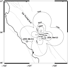
Figure 5. Parkfield region in central California showing four cGPS stations crossing the San Andreas fault. The contours indicate coseismic deformation caused by the 2004 Mw 6.0 Parkfield earthquakes (epicenter denoted by star) approximated by a global centroid moment tensor (CMT) solution (section 5.2.1). Also shown is the epicenter of the 2003 Mw 6.5 San Simeon earthquake. Prepared by Dara Goldberg.
Download figure:
Standard image High-resolution imageGPS time series analysis is subjective for several reasons and depends on the parameters of interest. Typically, parameters a (initial value), c-f (periodic terms), and h (non-coseismic offsets) are considered 'nuisance' parameters. Although there have been several attempts to automate the detection of non-coseismic offsets h (Williams 2003a), considerable manual effort is still required for reliable results. One could assign an offset parameter in all three components, for example, at any epoch when the GPS antenna has been replaced with one with different characteristics; a similar change in receiver is less likely to create a significant offset. Although it is good practice not to replace an antenna except when it needs repair, inevitably there will be changes; for example, modern GNSS antennas that can track both GPS and other satellite constellations are desirable. However, many continuous GPS stations have been operating for more than two decades with older instrumentation. The precision of the parameters of interest (e.g. the secular term coefficient b denoting the interseismic velocity) will degrade as the number of added offsets increases, so they should be kept to a minimum. Sometimes when an antenna change is planned, a temporary station is deployed nearby (<50 m) before and after the change to be able to estimate an accurate change in apparent position, which can be applied as a correction to the time series. This is not possible when an antenna unexpectedly fails. Often it is the case that before an antenna fails it will suffer degraded performance that is exhibited as an apparent wandering of the position or noisier model-fit residuals, which further complicates time series analysis. Assigning coseismic offsets is more straightforward; the complication occurs when deciding which stations have been significantly affected by an earthquake in a particular region. A model of the expected coseismic displacement field over a region can be obtained, e.g. from a centroid moment tensor solution for the earthquake source described in section 5.2.1 (figure 5), as a means of identifying stations that may have changed position above a certain threshold (typically 1 mm). Another complication is missing epochs when a station fails to collect data or collects poor quality data, which can create data gaps of varying length, and outliers. Furthermore, setting 'outlier' detection and rejection criteria is subjective; robust statistics (median, interquartile range) are useful to better distinguish outliers (Nikolaidis 2001). Finally, in the search for transient deformation (section 4.8) the main metric for setting detection criteria is the model post-fit residuals  (19).
(19).
3.3. Noise characteristics
Obtaining realistic estimates of model parameter uncertainties is fundamental to the identification, verification, and interpretation of physical signals. This is especially important when the magnitude of the underlying physical process is small against a background signal, e.g. identifying transient motion (section 4.8) that deviates from the simplified concept of the crustal deformation cycle, distinguishing differences between current-day tectonic plate motions estimated from geodesy and the long-term geologic record (section 4.3), or properly interpreting a geodetically-derived sea level rise attributed to anthropogenic climate change in the presence of natural variations (section 7). In this section, we discuss the nature of error  (44) in the daily GPS position time series.
In general, the power spectra of geophysical and atmospheric noise processes can be approximated by a power law process (Agnew 1992)

where  is the temporal frequency, k is the spectral index, and
  and
and  are the normalizing constants. A more general noise model is the Gauss–Markov process

where  is the crossover frequency, i.e. the point where the spectrum of low and high frequencies cross over, which is used quite often in GPS data analysis. The value of k for physical processes may range from k = 0 to k = −3 (Mandelbrot and Van Ness 1968, Agnew 1992). Special cases of integral spectral indices include white noise (k = 0), flicker noise (k = −1), and random walk noise/Brownian motion (k = −2). The spectral index is not limited to integer values. For example, Kolmogorov atmospheric turbulence has a range of spectral indices
 , which has been applied in studying the regional effects of troposphere refraction on geodetic observations (Williams et al 1998).
Experience with long records of terrestrial displacement measurements including spirit leveling (Karcz et al 1976), trilateration (electronic distance measurement) (Langbein et al 1987, Langbein and Johnson 1997) and tiltmeters (Wyatt 1982, 1989) indicate that there are significant temporal correlations in their respective time series, which could obscure or bias the underlying geophysical signal. In particular, power spectral analysis of their post-fit residuals  (19) resembles a random walk process (sometimes called 'red' or 'brown' noise) with a rise of
  . This has been attributed in these early studies to the instability of geodetic monuments caused by, e.g. expansive clays in near-surface rocks. However, as discussed later in this section, the power spectra of increasingly-long GPS displacement time series indicate that flicker noise (sometimes referred to as 'pink' noise) with a rise of
  may be more dominant. In any case, a good representation of noise
  has been found to be a combination of white noise and colored noise components with an appropriate choice of
  (Zhang et al 1997, Mao et al 1999, Williams et al 2004).
Consider then the simple case of a linear weighted least squares fit to a single component (e.g. the north component) of the displacement time series of n values,

Noise term  can be considered as a sum of uncorrelated errors (white noise, k = 0) due to instrument uncertainty and colored noise as represented by its covariance matrix of dimension n

with coefficients  for white noise and
  for colored noise, where I is the identity matrix and
  contains the frequency dependence. Again, the weighted least-squares inversion (19) for parameters
  (offset) and
  (velocity) yields

For a white noise process, bk = 0 and with no colored noise, covariance matrix  is a diagonal matrix with elements
  . The least-squares estimate for the station velocity error is then (Zhang et al 1997)
where n is the number of time series data points equally spaced in time and T is the total time span. For a random walk process, the covariance matrix is
The corresponding estimated variance for the station velocity is surprisingly simple (Zhang et al 1997)
indicating that unlike the white noise case (51), it depends solely on the time interval T between the first and last data points. In practice, the power spectra of the GPS time series have been found to be closer to flicker noise. In this case (Zhang et al 1997),
where element (i, k) of the symmetric matrix  of dimension n is
Note that there is no explicit reference to time or sampling frequency as flicker noise is on the asymptotic boundary between stationary and nonstationary processes and often exhibits odd behavior. There is no simple analytic expression for  for a flicker noise process. An approximate expression is given by (Williams 2003b),
An empirical formula for the estimation of the contribution of the colored noise component to station velocity uncertainty in the general case of fractal spectral index k is (Williams 2003b)

where

The term  is a polynomial of degree N with N + 1 coefficients (Williams 2003b). The effect of choosing an appropriate index on the rate uncertainty versus number of points is shown in figure 6 for a number of integer-valued spectral indices
  . The rate at which the uncertainties decrease as a function of number of points slows from 1/n3 for k = 0 and 1/n for k = −2, with nearly no decrease for k = −3. The crossover point for a particular spectral index is when the colored noise component
  starts dominating the white noise component
  of equal magnitude. The following expression denotes the number of data points n required for the colored noise to dominate the white noise,
where  is the cross over frequency and
  is the sampling frequency (Williams 2003b). Note that in all cases shown in figure 6 the colored noise dominates quickly.
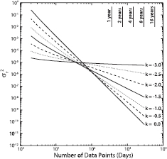
Figure 6. Velocity uncertainty variance  as a function of time for a range of spectral indices, assuming a sampling interval of once per day and a constant noise amplitude, bk = 0.001. From (Williams 2003b). Copyright 2003 with permission from Springer.
Download figure:
Standard image High-resolution imageThe variance coefficients  and
and  in (48) are often obtained through maximum likelihood estimation (MLE) of the displacement time series residuals assuming a certain power law (Langbein and Johnson 1997, Zhang et al 1997, Williams 2003b). One way to assign an appropriate spectral index
  and its uncertainty is by linear least squares fitting of the slope of the amplitude spectrum of the modeled displacement time series residuals (Zhang et al 1997). Once the spectral index and white noise and colored coefficients are determined, the proper covariance matrix
  can be then used in the weighted least squares inversion (49). The advantage of this approach is that all estimated model parameters (40) can be scaled properly. As the number of observations increases, a simpler and less time-consuming approach is to apply an empirical formula to properly scale the velocity uncertainties, which is often the primary parameter of interest (Williams 2003b). Other studies (Herring 2003, Bos et al 2008) have presented more efficient schemes for estimating velocity uncertainties in the presence of colored noise that, when the displacement time series are well behaved, approximate the more rigorous spectral approaches described above.
Estimates of the most appropriate spectral indices and the relative contribution of white noise and colored noise components have been obtained by several studies of daily displacement time series. Time series produced by several analysis groups encompassing nearly 1000 time series from 414 stations with time spans ranging from 16 months to a decade were analyzed using maximum likelihood estimation (MLE) (Williams et al 2004). For GPS stations that were globally distributed the optimal integer spectral index noise model (among k = 0, k = −1 and k = −2) was the white noise plus flicker noise (k = −1) model for all three components, confirming earlier studies with more limited data sets (Zhang et al 1997, Mao et al 1999). The results were similar when MLE was used to simultaneously estimate a non-integer spectral index, as well as the amplitudes of the power noise and white noise components. In both cases there were higher amplitudes in both the white noise and flicker noise components in the equatorial regions and in the southern hemisphere, as noted previously (Mao et al 1999). When using spatial filtering to reduce common-mode noise in regional-scale networks (section 3.5) the results were more varied but were centered about the white noise plus flicker noise model with significantly lower noise (smaller amplitudes in the colored and white noise terms); the white noise components were of the order of 0.5–1.0 mm in the horizontal components and 3.0 mm in the vertical component, while the flicker noise was on the order of  in the horizontal and
  in the vertical. With non-filtered, globally-distributed stations the noise was about three times larger in the horizontal components and five times larger in the vertical for both the white noise and flicker noise components. The white noise component varied between different analysis strategies, while the flicker noise was comparable, suggesting that the former is due to computational differences and the latter to underlying physical processes such as atmospheric noise (Williams et al 1998), second-order ionospheric effects (Kedar et al 2003), and seasonal atmospheric mass distributions (Dong et al 2002). The least noisy results in the study were for the two long-lived regional cGPS networks designed for plate tectonic studies in the western US, the Basin and Range GPS Network (BARGEN) and the Southern California Integrated GPS Network (SCIGN). In common for the two networks are uniformly stable monuments that consist of five deeply-anchored drill-braced stainless steel rods, a quincunx of one vertical and four slanted deeply-anchored (~10 m) monuments isolated from the surface down to ~3 m (figure 7) (Bock et al 1997). As noted previously, studies of noise from extremely sensitive tiltmeter and strainmeter observations for which the most stable monuments have been built (Wyatt 1982, Wyatt 1989) suggest a random walk process. These observatory instrument studies are the rationale for building the expensive deeply-anchored monuments for some geophysical networks to reduce the amplitude of this noise attributed to monument instability. Indeed other (relatively inexpensive) monument types (e.g. building mounts, metal tripods, rock pins, concrete slabs, concrete piers, and steel towers) indicate larger white noise and colored noise components, but with spectral indices lower than random walk for all monument types (Williams 2003b). The time series analyzed in the GPS studies may not be long enough to reveal an underlying random noise component. Ultimately, the overriding issue for anchoring in many locales is the hydrology or freeze thaw cycle over an area much larger than the footprint of the anchor. The BARGEN results are the least noisy, which is thought to be due to the dry desert conditions (Davis et al 2003). A third network, the US Pacific Northwest GPS Array (PANGA), had larger colored noise amplitudes thought to be due to the wetter atmospheric conditions and less stable monuments. Overall for this study, station velocity uncertainties were on the order of 0.05–0.1 mm yr−1 in the horizontal components and 0.2–0.3 mm yr−1 in the vertical; the contribution of the flicker noise was about 0.2 mm yr−5/4 for the horizontal components and 0.7 mm yr−5/4 for the vertical.

Figure 7. Two types of geodetic monuments. (Top) deeply-anchored drill-braced designed by Agnew and Wyatt—see figure 2; (bottom) shallow-anchored rock pin monument in bedrock. From (Bock et al 1997). Copyright 1997. This material is reproduced with permission of John Wiley & Sons, Inc.
Download figure:
Standard image High-resolution imageAn analysis of displacement time series of 256 stations from the BARGEN and SCIGN projects using a more selective set of filtered (section 3.5) daily position time series indicated the lowest white noise and flicker noise amplitudes with the preferred noise model being a combination of white noise and flicker noise with a random walk noise component (Langbein 2008). In this study, the flicker noise component was considered to be due to the GPS system itself (e.g. the receivers, satellites, local antenna environment) and fell in the frequency band between the high frequencies (white noise) and the low frequencies (random walk noise). Furthermore, this study suggested that the added expense of using expensive deeply anchored monuments (figure 7) may not have been justified, which is at variance with other referenced studies. Rather the location of the GPS monument is the overriding noise factor; sites in dry climates have less noise, while sites with anthropogenic effects (e.g. oil extraction and water extraction) have the most noise. Another study of data sets as long as 13 years indicated that flicker noise dominated in more than 70% of the daily station time series with white noise of 1.9 ± 0.1 mm and colored noise of 5.8 ± 0.1 mm yr−1/4. The effect on vertical velocity (1 − σ) uncertainty ranged between 0.1 to 3.3 mm yr−1 with a median value of 0.34 mm yr−1 (Santamaría-Gómez et al 2011). A study of seismic risk using 200 stations in the central US with up to 14.5 years of cGPS displacement time series indicated insignificant motions with an upper bound in strain accrual on faults of about 0.2 mm yr−1, within the 95% confidence limit of zero deformation. This result for the intraplate New Madrid Seismic Zone that experienced several large earthquakes up to a magnitude 8 in 1811–1812 held for 3 different combinations of white, flicker, and random walk noise models (Craig and Calais 2014).
Noise analysis of GPS position time series from global and regional stations is complicated by spatially correlated noise due to mis-modeling in the GPS analysis of phase and pseudorange measurements, in particular orbital and atmospheric errors, and limitations in the underlying terrestrial reference frame. Thus, studies of short baselines of less than 1–2 km are informative since residual regional and global effects are negligible, leaving only temporally correlated errors that are site dependent such as monument instability, multipath, and imperfect antenna phase center models (King and Williams 2009, Hill et al 2009). Noise levels for long baseline displacement time series are about an order of magnitude greater. Another advantage is that it is not necessary to form the ionosphere-free observable since the ionospheric effect is negligible so that measurement noise is reduced further by about a factor of 3 (12). On the other hand, the noise analysis is not site specific and includes the combined effects of the two baseline end points. Time series of relative displacements were analyzed for ten very short baselines from 1–140 m for the period 2000–2007 with various types of monuments, in different climates, with a variety of instrumentations (King and Williams 2009). They found that signal multipath, antenna phase center models, and elevation cutoff had negligible effects, so that the deviations of the time series from their mean value well represented monument motion. Time correlated noise mostly resembled a power law relationship with flicker noise dominating or a first-order Gauss Markov process (46); the amount of any random walk noise was constrained to be less than 0.5 mm/yr−1/2. Interestingly, some baselines had linear rates of >0.25 mm yr−1 and an annual signal >0.5 mm. The latter effect may be due to a combination of near-field multipath sources and changing satellite geometry, or actual monument motion; the former effect would contaminate studies of tectonic motion at the same level. The best monumented baseline at the Piñon Flat Observatory in southern California, with deeply-anchored monuments at both ends (figure 7) and in arid conditions, had no signal in annual or semiannual periods >0.1 mm and power law noise closer to random walk noise (k = −2) of order 0.2 mm yr−1/2; again, the presence of random walk noise in earlier studies of monuments was the rationale for installing deeply-anchored monuments. However, the analysis of this baseline was complicated by offsets in the data due to multiple changes in the GPS instrumentation. Other stations had noise values >0.4 mm with annual and semiannual periods. Another study was performed on short baselines (10–1000 m) in arid conditions in Nevada but using less than 3 years of data (Hill et al 2009). They found root mean square (RMS) residuals of 0.05–0.24 mm for the horizontal components and 0.20–0.72 mm in the vertical with seasonal cycles with amplitudes of 0.04–0.60 mm for all three components, which lag seasonal cycles by 23–43 d in local temperature measurements suggestive of bedrock thermal expansion. Interestingly, there is an increase in RMS with increasing station separation even at these short distances suggesting that site-specific effects are unlikely to be the limiting factor. As in a previous study (Langbein 2008), there was no difference between more expensive deeply-anchored braced monuments and shallow-based monuments. Despite the short data set (<3 years), MLE analysis indicated white noise plus colored noise with characteristics that fall between flicker noise and random walk, with mean power law indices of 1.4 ± 0.2, 1.5 ± 0.2, and 0.9 ± 0.3 for the east, north, and up components, respectively.
3.4. Seasonal effects
Seasonal, e.g. annual and semi-annual terms, in GPS time series (40) are due to physical processes such as non-tidal atmospheric loading and hydrological effects and other unmodeled effects in the inversion (19) of GPS phase and pseudorange observations for parameters of interest. Understanding seasonal effects is complicated by the possibility of the superposition of several noise sources. Their presence can be considered 'noise', which complicates assigning meaningful uncertainties to estimates of tectonic and seismic motions. Furthermore, the presence of seasonal effects necessitates longer data spans to extract the underlying crustal deformation parameters (e.g. station velocity). A study of the influence of annual signals on GPS-derived velocity uncertainties indicated that velocity bias rapidly becomes negligible after ~4.5 years; on the other hand, velocities from time series that are less than 2.5 years are seriously biased and should not be used for geophysical studies (Blewitt and Lavallée 2002). Based on increasingly long time series, the effects of periodic signals on velocity estimates is small (less than 0.2 mm yr−1) (Santamaría-Gómez et al 2011).
Dong et al (2002) investigated the possible sources of seasonal effects on 4.5 years of global GPS displacement time series and sorted them into three categories. The first is related to the gravitational attraction of the Sun and Moon, including seasonal polar motion, Earth rotation variations, and loading displacements due to solid Earth, ocean and atmospheric tides, and pole tide loading (section 2.5.1). The second category is related to hydrodynamics and thermal effects including atmospheric pressure loading, non-tidal sea surface fluctuations (Williams and Penna 2011), anthropogenic groundwater and mineral extraction, snow accumulation, local thermal expansion, and seasonal changes in the reflecting surface (soil moisture and vegetation) that produce multipath errors. The third category include effects specific to GPS analysis such as satellite orbital errors and choice of atmospheric models including mapping functions (section 6.1.2). For example, inadequacies in zenith delay mapping functions introduce significant periodic terms in annual and semiannual periods (Jin et al 2007). Typically, it is preferred to apply the physical model at the inversion step rather than apply parameteric fitting to the final displacement time series for annual and semiannual effects (section 3.2). For example, it has been shown that vertical surface displacements caused by atmospheric pressure loading are best accounted for in terms of the estimated heights of the stations at the time of the inversion of the observations, rather than applying time-averaged values to the coordinates after the analysis of the observations (Tregoning and van Dam 2005a, Tregoning and van Dam 2005b). For non-tidal atmospheric loading, a daily average is sufficient. The complication is for the diurnal and semi-diurnal thermal tides, which are currently not modeled well enough to be used in operational GPS analysis. The main sources of seasonal effects in the vertical direction, after the known sources of tidal effects and mass loading have been accounted for, are residual surface mass distributions from the atmosphere, oceans, snow and soil moisture, and pole tide loading. The amplitudes vary from 1–4 mm (Dong et al 2002).
Tidal forces, most predominant in semi-annual and annual periods, are modeled in the GPS data analysis (section 2.5.1). However, tidal-induced daily and sub-daily effects undersampled by daily (24 h) position time series alias the estimation of annual and semi-annual signals (Penna and Stewart 2003) due to the repeat period of the satellite orbits being longer than the Nyquist period of the semi-diurnal and diurnal tidal signatures. A ten year span of simulated data (Penna and Stewart 2003) and seven years of observed data (Penna et al 2007) showed that mismodeled tidal forces and undersampling with 24 h displacement time series can explain the annual and semi-annual signatures in GPS heights with amplitudes up to the several mm level, exhibiting long period signals from 12 d to one year. A study of the effects of mismodeled Earth tide effects on estimates of vertical positions found amplitudes of up to 0.4 mm for annual periods and 2 mm for semi-annual periods, increasing as a function of latitude, and 2 mm in zenith troposphere delay parameters (section 6.1.2) with a dominant diurnal frequency (Watson et al 2006).
Spectral analysis of weekly coordinate time series of global GPS data revealed the possible influence of the GPS draconitic year, the 351.4 d (draconitic frequency of 1.04 cycles yr−1) with which the GPS orbit repeats its inertial solar orientation (Ray et al 2008). The lower harmonics of the draconitic year are of annual and semiannual periods. Similar seasonal terms are not present in other space geodetic (very long baseline interferometry and satellite laser ranging) time series, implying that the annual and semiannual signals seen in GPS time series are related to orbital errors. Seasonal signals at the draconitic frequency may be due to climatic effects, specifically tidal atmospheric loading, which are magnified in ambiguity-free solutions compared to ambiguity-fixed solutions (Tregoning and Watson 2009). Multipath errors (section 8.4) can also manifest in seasonal signals at the same period through small variations in the satellite orbits (King and Watson 2010).
The seasonal signal itself may have a time dependence and neglecting the stochastic component may significantly affect the estimates of time-variable time series parameters such as velocities and their uncertainties by introducing correlations in the time series and a reddened power spectrum (Davis et al 2012b). This would be the case if the underlying noise of the seasonal signal (regardless of the cause) is colored, and they demonstrated that modeling a geodetic time series with constant amplitude sinusoidal terms (e.g. annual and semiannual) would still leave a strong stochastic signal in the time series residuals. For example, neglecting the stochastic seasonal component with a time series with a white noise (1.5 mm amplitude) and flicker noise process could underestimate the rate uncertainty by as much as 0.15 mm yr−1.
Annual signals present in the vertical component of geodetic time series can be due to solid Earth loading from continental (wavelengths greater than 100 km) water storage. Vertical signals are on the order of 8–30 mm yr−1. Resulting strain is manifested as tilts (20 nanostrains) and horizontal deformation (5 nanostrain) (van Dam et al 2001). On a regional scale, analysis of spatially filtered (section 3.5) daily displacement time series of stations in southern California with deeply-anchored monuments (figure 7) suggests that strain in the elastic part of the Earth's crust induced by surface temperature variations (thermoelastic strain) is a significant contributor to seasonal variations (Prawirodirdjo et al 2006). Other seasonal effects (anthropogenic, hydrological, and climate related) are discussed in section 7 in the context of climate change and in section 8 in terms of land subsidence.
3.5. Spatio-temporal filtering
Examination of the post-fit residuals,  (19) of the GPS displacement time series often reveals common non-tectonic signatures within a geographical region (e.g. the western US) indicating an external source of error. A simple spatio-temporal filter that removes the mean value at each time epoch for a set of regional stations results in significantly reduced noise characteristics in both white noise and colored noise amplitudes, allowing improved discernment of tectonic signals (Wdowinski et al 1997). The process to compute the common-mode error (CME) at epoch ti can be described by

where  is the residual value for a single coordinate component (ΔN, ΔE or ΔU) for station k and n stations and
  is its variance. Then at each epoch, the 'filtered' coordinate components
  have the common mode error removed from the original 'unfiltered' coordinate components
  by
by

This is usually performed in an iterative manner until all outliers, flagged according to criteria based on robust statistics (Nikolaidis 2002), are removed.
The spatio-temporal filtering approach can be generalized using principal component analysis (PCA) (Dong et al 2006). The demeaned and detrended post-fit residual time series are stored column-wise in matrix X according to each daily displacement component (ΔN, ΔE, ΔU) (37), in turn, for m days and n stations, assuming m > n. The 'covariance' matrix B is defined by

and applying singular value decomposition

B is a full rank matrix of dimension n, V is the eigenvector matrix with orthonormal rows and  has k non-zero eigenvalues along its diagonal (
 ). The eigenvalues λk and eigenvectors e(k) are sorted by descending order of the eigenvalues. The principal components, PC, for the kth mode are then given by the kth column,

The matrix X can be reconstructed as the superposition of the first k principal components
The largest principal component corresponds to the primary contributor to the variance of the network-wide residual time series, while the smallest principal component has the least contribution. The largest principal component may be the CME (61) or the postseismic signal (section 4.6), while the smaller ones may be related to local (e.g., hydrological, volcanic) or non-tectonic site-specific effects.
A modified version of the stacking procedure ((61) and (62)) using singular value decomposition was applied to post-fit residual GPS position time series on the North America plate with a focus on Mexico and the continental US (Márquez-Azúa and DeMets 2003). They found spatial coherence across a 2000 km scale with 95% of that within the first 1000 km. The stacking procedure was applied for each station, using all North America time series except for the station itself and the common mode error was computed for each station. A singular value decomposition of the resulting 174 common mode values indicates that two singular values make up 95% of the variance. Furthermore, they performed a singular value decomposition of the unfiltered residual time series and found that three singular values account for 45% of the variance reduction. The remaining ones indicate site specific noise, such as monument instability. Their conclusion is that 90% of the common mode error can be removed by applying two linearly independent sets of corrections. Furthermore, spatial filtering improves the precision of the station velocity estimates by a factor of two.
PCA analysis of GPS displacement time series, based on a combined analysis of individual time series estimated by the Jet Propulsion Laboratory and the Scripps Institution of Oceanography, now spanning 10–22 years for stations in the western US region consistently reduces the root mean square (RMS) of north, east, and up post-fit residuals by about 20–50%, from about 1–2 mm to 0.5–1.0 mm for horizontal components, and from about 3–5 mm to 2.5–4.5 mm in the vertical component.
4. Tectonic GPS and crustal deformation
4.1. Motivation
GPS measurements of surface displacement play a significant role in quantifying crustal deformation from the scale of single geological faults to global tectonic plate motions. The GPS has replaced traditional terrestrial geodetic techniques (triangulation and trilateration) because of its distinct advantages; it can measure over long distances without the requirement of line of sight between stations and it yields 3D positions with respect to an Earth-fixed, Earth-centered reference frame (section 2.5.3). This section describes the use of GPS and other geodetic data to contribute to and constrain models of physical processes in the solid Earth.
On a global scale, GPS displacement time series directly measure the relative motions of large rigid spherical lithospheric plates in motion according to plate tectonic theory (section 4.3). At regional scales, GPS measures deviations from plate tectonic theory in terms of plate boundary deformation. Tectonic plate boundaries are generally narrow along ocean ridges and transforms (from ~1 km to tens of km), but continental boundary deformation is often wide and diffuse across hundreds to thousands of kilometers, requiring many GPS stations for adequate spatial coverage. At the level of fault systems, GPS-derived displacements support the presence of a loading cycle, referred to as the 'earthquake cycle'. Simply stated, the cycle consists of steady interseismic motion driven by tectonic forces gradually accumulating stresses in the crust, episodic coseismic displacements partially relieving the stresses, and a postseismic phase when the crust and upper mantle return to the steady interseismic motion (figure 8, see also figure 14). Understanding the earthquake engine over many earthquake cycles and quantifying the state of stress in the crust falls within the realm of tectonic geodesy, in which GPS is playing an increasingly dominant role. Probabilistic models based on GPS and other data should considerably improve earthquake forecasting and perhaps, one day, play a role in prediction. However, the detection of premonitory seismic motions (precursors) remains elusive.
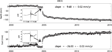
Figure 8. Detrended daily displacement time series for cGPS station MIDA in the Parkfield region, central California (figure 5) for the period 1999.5–2015.25, showing coseismic and postseismic deformation caused by the 28 September 2004 Mw 6.0 Parkfield earthquake. The white line through the daily positions is the weighted least squares model fit (40). The Parkfield earthquake's epicenter was ~18 km SE of MIDA (figure 5). Note the coseismic offset in late 2003 is due to the 22 December 2003 Mw 6.6 San Simeon earthquake ~90 km WSW of MIDA. Both earthquakes were fit with a logarithmic function (41) with decay times of 5 and 10 d, respectively, to account for postseismic deformation. The map inset shows coseismic displacements (static and dynamic) at a rate of 1 Hz for the duration time of the Parkfield earthquake analyzed with the PPP-AR method (section 2.4.2); the horizontal scale is UTC time and the vertical scale is centimeters. The peak to peak dynamic motion is about ~10 cm in the north component and ~8 cm in the east component. The uncertainties for the velocity components denote one standard deviation based on a white noise plus flicker noise model (56). Prepared by Jianghui Geng and Lina Su.
Download figure:
Standard image High-resolution imageDeviations from the simple notion of a crustal deformation cycle and steady uniform fault motion have also been directly observed by GPS at a range of spatial and temporal scales. One of the early observations of along-fault variations in interseismic motion was made as part of a study of oblique subduction of the Indian plate at the Java trench off Sumatra, with the Sunda Shelf (Prawirodirdjo et al 1997). This phenomenon is now seen in many tectonic settings, where strain segmentation along active faults indicates variations in fault coupling. Transient deviations were observed through analysis of cGPS displacements, including afterslip and slow-slip ('silent') events, first in Japan (Hirose et al 1999) and in Cascadia (Dragert et al 2001). Slow-slip events accompany deep seismic signals known as tremor, and together are called episodic tremor and slip (ETS) (Rogers and Dragert 2003), as described in section 4.8.
Present-day surface velocities measured by GPS provide a measure of crustal strain from which fault slip rates can be determined. When combined with available historical records and paleoseismic dating of earthquake recurrence, these are indicative of the rate of strain accumulation for a particular fault segment or fault system. This information is useful for assessing the probability that a major earthquake will occur within a certain period of time. Fault segments with significant strain accumulation that have not ruptured in a recent earthquake compared to neighboring segments or that experience migrating earthquakes and transfer of stress are of particular concern for seismic hazard. For example, 'slip deficits' along the North Anatolian fault/Marmara fault system (Stein et al 1997, Pondard et al 2007) have been suggested to be likely locations for large earthquakes. However, this basic model has been modified as it has become evident that adjacent segments can have different degrees of fault coupling and that aseismic slip can reduce accumulated strain available for earthquakes.
The 2004 Mw 9.3 Sumatra–Andaman earthquake brought into question some of the basic assumptions concerning subduction zone earthquakes (Subarya et al 2006). For example, at the Mariana style subduction zones the subducting plate is old, and thus cold, and it sinks readily into the mantle. As a result, the coupling at the subduction front should be low and few large earthquakes are produced. In contrast, Chilean-type subduction zones, where the subducting plate is young, warm, and buoyant, should have higher coupling and an abundance of large events as the incoming slab resists subduction (Stern 2002). However, the unexpected occurrence of the 2004 Sumatra–Andaman event on the northern end of the Sumatra subduction megathrust, over a distance of 1500 km and a width of 150 km with a magnitude of Mw 9.1–9.3, contradicted the hypothesis that the maximum earthquake magnitude on a given thrust increases linearly with the convergence rate and decreases linearly with the subducting plate age (Molnar et al 1979, Uyeda and Kanamori 1979). Here the subducting lithosphere is old and converging at a moderate rate and there is only evidence of lower magnitude events (Subarya et al 2006). The occurrence of several great subduction-zone earthquakes in regions that were thought to be unlikely (the latest example being the 2011 Mw 9.0 Tohoku-oki, Japan earthquake) based on the relatively short historical record indicates that any subduction zone is a candidate for a great event whose size is limited only by the available area of the locked fault plane (McCaffrey 2008). The widespread availability of GPS velocity fields has facilitated systematic studies of strain accumulation, plate coupling, and transient motion at different styles of subduction zones and probing of the relative importance of the different mechanisms ongoing at a subduction zone (Wallace et al 2009).
Postseismic deformation is an important indicator of crustal dynamics, and is discussed in section 4.6. It can be long-lived after large earthquakes and span several decades. It was found that even after 40 years, the GPS velocities in the region around the great 1964 Mw 9.2 Alaska earthquake were still affected by the postseismic relaxation of the crust and underlying mantle (Suito and Freymueller 2009). Similarly, the present day velocity field is still showing the postseismic effects of the 1960 Mw 9.5 Valdivia, Chile earthquake (Wang et al 2012). The physical mechanisms controlling postseismic deformation may differ from earthquake to earthquake. The underlying assumption is that station velocities are the same through several earthquake cycles; however, there have not been enough geodetic data collected to date to verify it. This fundamental difficulty can be partially overcome by comparative studies of plate boundaries that are in different stages of the earthquake cycle. These studies have benefited from the widespread deployment of cGPS stations at many plate boundaries. For example, the subduction zones in Sumatra, Chile, and Cascadia are in three different stages of the earthquake cycle (Wang et al 2012). In Sumatra, observations from one year after the 2004 Mw 9.3 earthquake showed most of the sites continued to move in the same directions as coseismic motion. This is indicative of afterslip (section 4.8.2) dominating the kinematics. Meanwhile in Chile, 40 years after the 1960 Mw 9.5 Valdivia earthquake, coastal and inland sites were found to have opposing motions due to the mantle still undergoing postseismic relaxation. Finally, in Cascadia all sites were found to be moving landward as a result of a perfectly locked fault. These types of comparative studies provide estimates of the timescales to be expected for the viscous relaxation times of the upper mantle; importantly they also show that these times are expected to scale with seismic moment since they depend on the initial stress perturbation (the seismic moment is a measure of the size of an earthquake, based on the moment magnitude scale Mw).
In the following sections, we show how GPS displacement time series record all phases of the deformation cycle (figure 8) within the overall plate tectonic framework and how they complement measurements by other geodetic systems as well as data from geology, paleoseismology, remote sensing, and seismology. After a brief history, we order our discussion from global to local phenomena, moving from longer to shorter temporal scales. We review plate motion models and supporting data in section 4.3. In section 4.4, we discuss conceptual models of interseismic deformation, followed by models for fault slip at depth for single faults to large plate boundary zone fault systems, and the estimation of velocity and strain-rate fields in section 4.5. In section 4.6 we present postseismic deformation as a way to understand crustal rheology and fault mechanics. In section 4.7 we discuss coseismic displacements as input to models of the earthquake source. We conclude in section 4.8 with an overview of transient deformation that elucidates significant variations to the simplified paradigm of the earthquake cycle.
4.2. History
The connection between earthquakes and faulting was first inferred from observations of surface faulting related to the 1872 Owens Valley earthquake and geological mapping of the Great Basin in California (Gilbert 1884, Scholz 2002). Further geological observations of fault scarps after earthquakes in New Zealand (McKay 1890) and Japan (Koto 1893) supported the relationship between earthquakes and faulting. The first direct measurements of crustal deformation were serendipitously made on the island of Sumatra in the 1890s, when an Mw 7.6 right-lateral strike-slip earthquake occurred on a segment of the 1600 km long Great Sumatra fault (Prawirodirdjo et al 2000) during the course of repeated triangulation surveys by the Dutch colonial government (Müller 1895). Triangulation is an early surveying technique that measures angles between survey monuments with optical instruments after a short baseline is measured with an invar tape to determine network scale. It requires line of sight, thus preference is given to observations on high ground where available, and to tall towers when not. In this case, the Dutch surveyors took advantage of the peaks of the Bukit Barisan Mountains, a volcanic chain through which runs the Great Sumatra strike-slip fault. In the mid-20th century, triangulation was augmented by electromagnetic distance measurements ('trilateration') and was used extensively for crustal deformation surveys (Savage and Burford 1973). Today, 'total station' instruments, a combination of optical and electronic distance sensors, are still used for mapping, e.g. by land surveyors and archeologists.
The elastic rebound theory was developed partly based on Müller's work (Reid 1913) and triangulation measurements of surface offsets after the devastating 1906 ~Mw 7.9 San Francisco earthquake (Lawson and Reid 1908, Reid 1910, 1911). This earthquake was attributed to a rupture of the San Andreas fault, as part of an earthquake loading cycle consisting of elastic strain accumulation prior to an earthquake followed by sudden strain release. The idea that earthquakes represent an elastic reaction of the Earth's crust was first proposed by Hooke in his Discourse on Earthquakes lectures in 1667–1700 (Rappaport 1986). The elastic rebound theory, despite its simplicity, still serves as a useful paradigm for crustal deformation cycle studies and earthquake forecasting through estimation of fault slip.
4.3. Plate motion models
Tectonic plate motions are responsible for large-scale natural features such as continents, ocean basins, mountain ranges, and volcanoes, and natural disasters such as earthquakes, tsunamis, and volcanic eruptions. Earthquake belts, such as the circum-Pacific seismic and volcanic belt (the 'Ring of Fire'), are a direct manifestation of tectonic motion and coincide with plate boundaries and active geologic faulting. The Earth's lithosphere (outermost shell including the crust and upper mantle) is broken up into nine major tectonic plates, ten minor plates, and numerous micro-plates that are in relative horizontal motion with three general types of plate boundaries: (1) transform, or lateral—juxtaposing continent-continent, or ocean-ocean crust; (2) convergent (subducting)—juxtaposing continent-continent, ocean-continent, ocean-ocean crust; and (3) divergent—at continental rift and mid-ocean ridges. Generally, plate motion is modeled by the rotation of an aspherical rigid shell (the plate) around a pole of rotation with some angular velocity defined by a 'Euler' vector. The first plate motion models were derived from mid-ocean ridge spreading rates inferred from magnetic lineations, transform fault azimuths, and earthquake slip vectors (Minster et al 1974, Chase 1978). The magnetic data provided the time scale of plate motion over geologic time, and the transform fault azimuths and the earthquake slip vectors delineated the direction of motion. Based on the last geomagnetic reversal in the Pliocene, 'current' plate motion models provide representative values over the last 3 Myr. Since the plates move in relative motion over the entire Earth's surface, there is no obvious underlying 'Earth-fixed' reference frame. Thus, early models imposed a geometric condition that the plates have no net rotation (Solomon and Sleep 1974) or a physical condition based on the fixed hot spot hypothesis (Wilson 1963, 1965, 1973, Morgan 1971, 1972, Minster and Jordan 1978). Hot spots are areas of increased magmatic activity and heat flow due to upwelling of mantle material that are manifested by an alignment of shield-type volcanoes on the seafloor indicating the direction of relative motion of the overriding tectonic plate. Large amounts of energy are transported from the Earth's interior to the surface at hot spots and they are thought to result from mantle plumes originating either at the core-mantle boundary or within the mantle. There are 20–30 hotspots, mostly beneath the oceanic crust, and they are distant from plate boundaries; hence, they are a convenient tie to a reference frame independent from the moving plates. Significant refinements in global plate motion models were made as new data became available and older data were reinterpreted. Most seminal was the relative motion NUVEL-1 model composed of 12 rigid plates (DeMets et al 1990). The NUVEL-1 plate motion model was used to introduce a no-net-rotation requirement of the lithosphere, yielding the 'absolute' No-Net-Rotation (NNR) model, which significantly differed from previous hot spot models (Argus and Gordon 1991). A recalibrated version of NUVEL-1 was NUVEL-1A (DeMets et al 1994), which took into account changes in the geomagnetic reversal time scale by applying a scaling factor to reduce the plate velocities by about 5%, which agreed better with current velocities obtained with space geodetic methods, including very long baseline interferometry (VLBI) and satellite laser ranging (SLR) (Robbins et al 1993).
Morgan (1968) pointed out in the first paper on global plate motions: 'If the distances between Guadalupe Island, Wake Island, and Tahiti, all within the Pacific block, were measured to the nearest centimeter and then measured again several years later, we suppose these distances would not change.' Even earlier, Wegener the main proponent of 'continental drift' (Wegener 1912) wrote about geodesy's role in its verification, 'I have no doubt that in the not too distant future we will be successful in making a precise measurement of the drift of North America relative to Europe' (Wegener 1929). It took nearly 50 years for Wegener's concept of 'continental drift' and 20 years after the advent of plate tectonic theory to directly measure plate motions by geodetic methods. The first direct measurements were provided by global space geodetic data collected by the National Aeronautics and Space Administration (NASA) Crustal Dynamics Project (CDP) from repeated multi-year estimates of the position of global tracking stations by SLR (Christodoulidis et al 1985, Smith et al 1994) and VLBI (Herring et al 1986). These 'instantaneous' estimates (made over a decade) were compared to the ~3 Myr record and showed agreement within the uncertainties of the geodetic measurements for the major plates, thus supporting the rigid plate hypothesis. The first estimates of Euler vectors were derived from about 10 years of NASA CDP space geodetic data for Pacific–North America motions using VLBI and SLR stations within the interiors of the Pacific and North America plate (Argus and Gordon 1990, Ward 1990, Robbins et al 1993).
Expensive and geographically sparse space geodetic measurements using VLBI and SLR were gradually replaced by the GPS in the mid-1980s. Precise positioning required a network of permanent global GPS stations observing continuously to track the GPS satellites to be able to estimate precise satellite orbits with respect to a terrestrial reference frame (section 2.5.3). The changes in positions of these stations over time could also be used to further verify the underlying principles of plate tectonic theory (steady horizontal motion of a small number of rigid plates) and improve plate motion models. Early determinations of contemporary plate motions and comparisons with plate motion models used relatively short GPS data sets at a time when data analysis and infrastructure were still improving. Relative Euler vectors were estimated from 2–4 years of GPS data for six major plates and deformation at several locations within plate boundary zones, indicating general agreement with NUVEL-1A (at an uncertainty of about 2 mm yr−1), but with larger velocities for the relative motion between the Pacific plate and the Eurasia and North America plates (Argus and Heflin 1995). An analysis of selected global GPS data collected within the interior of eight major plates from 1991 to 1996 found general agreement with NNR NUVEL-1A velocities within the GPS uncertainties (1–5 mm yr−1), except for some differences in the poles of rotation and plate rates for the Pacific and Nazca plates (Larson et al 1997). A study of the Pacific-North America plate motion using cGPS observations from 21 stations concluded that the rotation rate has been steady since 3.16 Ma, but at rates significantly faster, by several mm yr−1, than predicted by NUVEL-1A (DeMets and Dixon 1999).
The ubiquity of GPS observations at an increasing number of well-distributed regional and global stations, longer spans of data, better reference frames, and improved analysis techniques provided a means to test the hypothesis of rigidity assumed by plate tectonic theory and the assumption of steady state motion by comparing short-term GPS-derived plate motions with the long-term geological record. Mostly GPS velocity data from 1993 to 2000 were used (Sella et al 2002) to develop a plate motion model ('REVEL') for 19 plates and continental blocks that demonstrated some significant deviations from plate motion models that were real and/or reflected limitations in the geological models, or were contaminated by possible earlier systematic errors in the GPS analysis. The North America, Eurasia, and Antarctica plates exhibited departures from rigidity due primarily to glacial isostatic adjustment (GIA) effects (section 7.4). Present day slowing compared to geologically-based plate motion models was attributed to long-term deceleration associated with continental collision for Arabia–Eurasia, Arabia–Nubia and Eurasia–India, and the slowing of Nazca–Pacific, Nazca–South America, and Nubia–South America due to the beginning of the current phase of Andean crustal shortening. The 'MORVEL' plate motion model (figure 9) consisting of Euler vectors and boundaries for 25 plates covering 97% of the Earth's surface used new data including GPS velocities, earthquake slip vectors, shipboard soundings (multi-beam and side-scan sonar) of bathymetry and dense magnetic surveys of the mid-ocean ridge system (Demets et al 2010). The GPS velocity data were also used to describe the motion of six smaller plates. MORVEL's primary goals were to produce the best available geologically-based plate motion model with respect to which geodetically-based observations could be compared and to provide a means to test one of the basic assumptions of plate tectonic theory; that the plates have no internal deformation. The study concluded that there are still significant differences between geologic and geodetic data, e.g. the relative motion of the North America and Pacific plates. Possible reasons were wider zones of diffuse deformation for the North America, South America, and other plates, a small anticlockwise change in North America and Pacific motion over the last 1–3 Myr, and internal plate deformation possibly caused by thermal contraction. As studies delved deeper with more and longer observations over space and time with lower uncertainties, the discrepancies with plate motion models became more apparent, that is, plate motion theory was deemed by direct observation as a useful first-order approximation for the Earth's deformation but state-of-the-art observations required increased complexity.
One of the difficulties in making geodetic comparisons with plate models is deciding whether the GPS stations are within the stable plate interior or not. For example, there is only a single land mass that rises above sea level on the Cocos plate (Isla del Coco). Survey mode (sGPS) and cGPS observations on the island indicated a convergence rate of 78 mm yr−1 with respect to the neighboring Caribbean plate (Protti et al 2012). This agreed well with the MORVEL model and indicated that, serendipitously, this site is on the rigid interior of the plate. Similarly, the Pacific plate, which is also almost completely under water, has few suitable land masses for GPS observations, with the added complexity that many of these are near clearly deforming plate boundaries (e.g. New Zealand, California), where rigidity is a poor assumption. It was determined from GPS observations that Guadalupe Island off the coast of Baja California was on the Pacific Plate while the Channel Islands off the coast of southern California were not (Gonzalez-Garcia et al 2003). This study took up the suggestion posed by Morgan (1968) by measuring the relative velocity between Tahiti and Guadalupe Island using GPS data collected from 1991–2002; it was indeed unchanged and the velocities of six GPS stations defined a Euler pole that was consistent with other geodetically-derived plate models, within a precision of about 1 mm yr−1. Another study examined 11 years of GPS data from global tracking stations and stations on the Pacific, North America, and the Australia plates (Beavan et al 2002). It found that the Pacific and Australia data fit a rigid relative plate model with a root mean square (RMS) velocity of 0.4 mm yr−1, and fit the North America and Pacific plate data with an RMS velocity of 0.6 mm yr−1. The stations offshore southern California differed from the Pacific plate motion by 4–5 ± 1 mm yr−1 and some stations in New Zealand indicated velocity discrepancies of 3 ± 1 mm yr−1, indicating that the plate boundaries were wider than previously believed. An examination of GPS data in the nominally rigid interior of North America from 300 stations collected over a 12 year period (1993–2005) found ~0.8 mm yr−1 of residual horizontal deformation corresponding to strain rates (section 4.5.5) of 10−9 yr−1 (Calais et al 2006). It attributed most of this deviation to glacial isostatic adjustment (section 7.4) and not to any tectonic source even in the New Madrid Seismic Zone, which experienced a series of large intraplate earthquakes (according to the US Geological Survey ~Mw 7.2 to ~Mw 8.1) in 1811–12. The GPS study of glacial isostatic adjustment in North America (Sella et al 2007) was consistent with the other studies (Calais et al 2006, Beavan et al 2002). Likewise, another study (Nocquet et al 2005) found the interior of the Eurasian plate in Europe to be rigid at the level of 0.6 mm yr−1, with deviations due mainly to glacial isostatic adjustment. These studies resulted in a clearer delineation of stable plate interiors versus deforming plate boundary zones.
4.4. Conceptual end member models for crustal deformation
As plate tectonics is to first order the underlying paradigm for explaining crustal motion and deformation is clearly located on faults, it is tempting to describe plate boundary deformation by rotating rigid microplates. The first conceptual models within the framework of plate tectonic theory were applied to the motion of rigid elastic blocks (small plates to microplates) to explain deformation in eastern and central Asia (Tapponnier et al 1982, Avouac and Tapponnier 1993, Peltzer and Saucier 1996) and rotating and translating blocks in Greece, New Zealand, and western North America (Lamb 1994). One study extrapolated laboratory rock experiments with plasticine (rather than strictly rigid elastic blocks) to explain non-steady state deformation of the continental lithosphere in the formation of extensional basins, such as the South China Sea, the North China Basin, and the Andaman Sea, near active strike-slip faults (Peltzer and Tapponnier 1988). By comparing plate rates to seismic moment release rates in western North America, the block motion model was preferred (King et al 1994a). The rise of the Tibet Plateau based on Cenozoic deformation, magmatism, and seismic structure was explained by time-dependent localized shear between lithospheric blocks, rather than a continuum model of crustal thickening and widespread flow of the crust and upper mantle (Tapponnier et al 2001). At the other extreme, crustal deformation can be considered as a continuum much like the flow of a viscous substrate with uniform rheology derived from basal shear with internal straining within the plates rather than block-like elements, so that faulting within deforming zones is smoothed over. This model was first proposed based on numerical and laboratory experiments for the India–Asia collision (England and McKenzie 1982, England and Houseman 1986, Molnar 1988a) and later with GPS (England and Molnar 2005). It is motivated by the existence of plate boundary zones of wide extent such as India/Asia (~2000 km) and Africa/Europe (~1000 km) (England and Mckenzie 1982), and the realization that continental interiors are not well explained through a plate tectonic model (Molnar 1988b). The view that large-scale processes in the continental lithosphere (buoyancy forces) are enough to explain the wide variety of rates and styles of observed deformation at plate boundaries was argued from estimates of gravitational potential energy and available rheological constraints in orogenic belts of the Western US geodetic data (GPS, trilateration, triangulation) collected in New Zealand and southern California (Jones et al 1996, Bourne 1998). That is, crustal blocks passively follow the long-term pattern of ductile deformation in the lower lithosphere and drive the accumulation of strain in the brittle upper crust, where faulting occurs. If so, then this should be reflected in the geodetically-determined measurements and the relative motion of crustal blocks can be predicted, so that the geodetic and geologic slip rates should match. However, actively deforming regions of the western United States, central Asia, Japan, and New Zealand showed features that argued for both styles of motion (Thatcher 1995).
Early studies of crustal deformation were limited by the amount of geodetic data available and complicated by apparent postseismic effects (section 4.6); regions experiencing postseismic deformation were just avoided. As an example, based on a velocity and strain field derived from geodetic measurements (VLBI and GPS), Quaternary fault data and the NUVEL-1A plate motion model, a diffuse model of extensional deformation with buoyancy forces within the Basin and Range and California shear zone lithosphere in the presence of relative plate motion forces was hypothesized, assuming insignificant basal tractions to derive the deviatoric stress tensor field (Flesch et al 2000). In going from strain rate to stress, they assumed an isotropic relationship, thereby excluding observed strain rates along the San Andreas fault since the directions of principal strain rate and inferred directions of principal stress were known to differ (Zoback 1992). GPS velocity fields in a variety of tectonic settings (transform, subduction, collision) in the Western US, New Zealand, Japan, and Greece suggested a model consisting of narrow zones (~10–100 km) of deformation interleaved with larger inactive blocks (Thatcher 2003).
4.5. Interseismic deformation
4.5.1. Background.
Quantifying the complex deformation at plate boundaries within the first-order context of plate tectonic theory is critical to understanding the underlying physical Earth processes, such as mantle convection and lithospheric dynamics, which drive the earthquake cycle, and fault mechanics, which explains the response of the crust. This knowledge is critical for earthquake hazard assessment to mitigate risks to society. Physical models seek to explain the kinematic description of crustal motions by GPS velocity vectors at discrete points, and will be presented in an order of increasing complexity. In the case of a single locked fault, at distances greater than one or two fault depths away from the fault the GPS velocities increasingly describe the interseismic tectonic plate rate. On the other hand, at closer distances, a simple model for the deformation of an elastic crust over a slipping fault at depth explains the first order change in surface velocity across the fault. This approach has been applied, for example, to the San Andreas fault at the boundary of the North American and Pacific plates. By dividing the crust into many crustal blocks, this simple model can be extended to describe a more complicated plate boundary fault system. The blocks may be rotating and the degree of coupling at the fault may vary, in addition to the locking depth of the fault. Finally, to explain observed deformation over the broadest plate boundaries, the lithosphere can be considered a continuum and strain rate is derived from the interseismic velocities. In each case, the accumulated strain described by the changes in kinematic velocities have implications for the earthquake cycle and potential for strain release determining the magnitude of earthquakes. Later we will see that even these increasingly complex models have been simplified by assuming that the Earth's lithosphere (and faults) behaves like an elastic-brittle solid, while the latest research shows that there may also be a continuum in the mechanical behavior of the faults.
As a first step, it is critical to measure the steady secular motion (interseismic deformation) that builds up stresses in the lithosphere as part of a cycle that repeats over many earthquakes, and which is the topic of this section. Field geology infers long term (~3 Myr) fault slip rates by surface mapping and observation of offset features, and documenting coseismic surface rupture. Paleoseismology documents the occurrence and frequency of earthquakes in the last 1–2 Kyr by trenching across active faults and dating exposed material disrupted by seismic events (Sieh 1978, Kumar et al 2006). Other information about earthquake recurrence over multiple cycles comes from archaeoseismology up to ~3Kyr in select locations (Nur and Ron 1996, Nur and Cline 2000), where damage observed in ancient cities can be attributed to earthquakes, paleogeodesy (coral uplift rates in subduction zones—Sieh et al 2008) and geomorphology (Ludwig et al 2010), all showing fault motion evidence in surface features. About 100 years of seismological observations provide a record of earthquakes, foreshocks, aftershocks, and microseismicity to infer fault geometry and depth, and provide additional information on the present day direction of slip. Interpreting crustal deformation at the surface driven by a process at depth is aided by studies of rock mechanics, which seeks to extrapolate information collected in the laboratory on small rock samples to fault zones. Early geodetic data, up to two centuries old and collected through triangulation and trilateration, e.g. in California (Lisowski et al 1991), Sumatra (Prawirodirdjo et al 2000), and Greece (Ambraseys et al 1990, Billiris et al 1991), have also provided useful observations. In the context of interseismic deformation, the primary value of the GPS is accurate direct measurements of aseismic secular motions of the strain buildup (strain rates), complementary to seismic observations that are limited to dynamic motions related to strain release (in section 5.2.3 we will discuss GPS seismology). GPS observations have been available since the early 1980s and have provided point measurements at thousands of ground stations throughout the globe, but have been particularly useful in their concentrated deployment at plate boundaries. A complementary geodetic technique is satellite-based interferometric synthetic aperture radar (InSAR) (Massonnet and Feigl 1998) and point scatterers (Ferretti et al 2001), which can detect surface deformation with much higher spatial resolution than the GPS, but with less temporal resolution due to the multi-day satellite repeat cycle; furthermore, they only provide relative motion. GPS positions in the satellite's swath are often used to tie the interferometric radar images to an absolute terrestrial reference frame (Bock et al 2012a). Radar interferometry is limited when ground surface changes between passes preclude extracting displacement signals due to decorrelation; for example, they do not perform well over agricultural areas. GPS and InSAR observations are, of course, only useful where land masses are accessible. Seafloor positioning is the most recent geodetic method that holds great promise for extending geodetic measurements to offshore faults across submerged plate boundaries. Seafloor geodesy ties displacements of reference markers with acoustic transponders deployed on the ocean bottom to the global terrestrial reference frame through GPS deployed on ships and buoys on the ocean surface (figure 10) (Spiess et al 1998, Sato et al 2011, Bürgmann and Chadwell 2014).
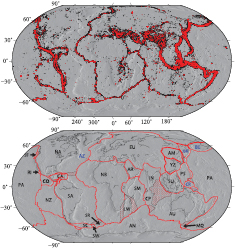
Figure 9. MORVEL plate motion model. (Top) Epicenters for earthquakes with magnitudes equal to or larger than 3.5 (black) and 5.5 (red) and depths shallower than 40 km for the period 1967–2007. Hypocentral information is from the US Geological Survey National Earthquake Information Center files. The patterned red areas show diffuse plate boundaries. (Bottom) Plate boundaries and geometries employed for MORVEL. Plate name abbreviations are as follows: AM, Amur; AN, Antarctic; AR, Arabia; AU, Australia; AZ, Azores; BE, Bering; CA, Caribbean; CO, Cocos; CP, Capricorn; CR, Caroline; EU, Eurasia; IN, India; JF, Juan de Fuca; LW, Lwandle; MQ, Macquarie; NA, North America; NB, Nubia; NZ, Nazca; OK, Okhotsk; PA, Pacific; PS, Philippine Sea; RI, Rivera; SA, South America; SC, Scotia; SM, Somalia; SR, Sur; SU, Sundaland; SW, Sandwich; YZ, Yangtze. The blue labels indicate plates not included in MORVEL. Reproduced with permission from figure 1 in DeMets et al (2010). Copyright 2010 The Royal Astronomical Society.
Download figure:
Standard image High-resolution image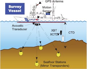
Figure 10. Schematic of a GPS/acoustic seafloor positioning system. CTD-conductivity-temperature-depth profiler; XCTD-expendable CTD; XBT expendable bathythermographs. Adapted from Sato et al (2013), copyright 2013. This material is reproduced with permission of John Wiley & Sons, Inc.
Download figure:
Standard image High-resolution image4.5.2. Velocity observations.
As GPS observations have proliferated, they have provided unprecedented clarity to the complex nature of crustal deformation. The first GPS surveys for crustal deformation (Feigl et al 1993), conducted from 1984–92, focused on the San Andreas fault system in central and southern California, a transform plate boundary zone dominated by the San Andreas fault, which includes other major and minor sub-parallel strike-slip faults (Elsinore, San Jacinto), as well as compressional features at major bends in the San Andreas. This project was focused on resolving the so-called 'San Andreas discrepancy' (Minster and Jordan 1984); subtracting a vector for the direction and rate of slip on the San Andreas fault from the velocity vector of Pacific/North America motion yielded a discrepancy of about 9 mm/yr. The 'discrepancy' was later resolved by extending the zone of deformation from the islands offshore California, through the Walker Lane in Nevada, and to the extensional Basin and Range province in the western US (Larson and Webb 1992), thus revising relative plate motion estimates. Subsequently, GPS geodesy has been instrumental in quantifying the kinematics of present day tectonic deformation. GPS-derived velocities representing small-scale to large-scale interseismic deformation have been determined across most of the Earth's plate boundaries, mostly through intensive and often challenging repeated field GPS surveys (sGPS), and later with growing numbers of permanent (cGPS) networks (section 2.1). These efforts are too numerous to discuss in detail but a representative list sorted by geographic location and tectonic setting is given in table 1 and three examples are discussed below. To get a sense of the extent and magnitude of the totality of efforts to date, it is useful to review the input velocity data sets to recent studies of global strain (Kreemer et al 2014).
Table 1. Representative list of crustal deformation studies with GPS sorted by geographic region.
| Region | Studies |
|---|---|
| Pacific /North America | McCaffrey (2005, 2009), McCaffrey et al (2007), McCaffrey et al (2013) (figure 12); Márquez-Azua and DeMets (2003), Freymueller et al (2008), Elliott et al (2010), Thatcher et al (1999), Dixon et al (2000), Bennett et al (2003), Blewitt et al (2009a) and Shen et al (2011) |
| Nazca/South America | Bevis et al (2001), Brooks et al (2003), Bejar-Pizarro et al (2013) and Nocquet et al (2014) |
| South America/Scotia | Smalley et al (2003, 2007) |
| Caribbean plate | Weber et al (2001), Lopez et al (2006), Manaker et al (2008) and Calais et al (2010) |
| India/Eurasia | Bilham et al (1997), Larson et al (1999), Paul et al (2001), Jade et al (2007), Gahalaut et al (2013) and Liang et al (2013) |
| Africa/Eurasia | Stamps et al (2008), Kogan et al (2012), Fernandes et al (2013), Saria et al (2013) and Saria et al (2014) |
| Mediterranean Africa/Eurasia | Reilinger et al (2006) (figure 11), Serpelloni et al (2010), D'Agostino et al (2011), Reilinger and McClusky (2011), Koulali et al (2011), Sadeh et al (2012), Echeverria et al (2013) and Muller et al (2013) |
| Southeast Asia | Bock et al (2003), McCaffrey et al (2006), Nugroho (2009) and Duong et al (2013) |
| South Pacific | Bevis et al (1995), Tregoning et al (1998), Calmant et al (2003) and Bergeot et al (2009) |
| New Zealand | Beavan et al (1999), Beavan and Haines (2001), Beavan et al (2010) and Denys et al (2014) |
| Australia/Sunda | Tregoning et al (1994), Tregoning (2002) and Wallace et al (2004) |
| Japan | Sagiya et al (2000), Nishimura et al (2004), Hashimoto et al (2009), Liu et al (2010a), Ohzono et al (2011), Tadokoro et al (2012), Sato et al (2013) (figure 13) and Yoshioka et al (2013) |
| Mexico and Central America | Iinuma et al (2004), LaFemina et al (2009), Plattner et al (2007), Márquez-Azua and DeMets (2009), Alvarado et al (2011) and Franco et al (2012) |
After a constant plate motion vector is removed from GPS velocities, it becomes clear that a model is required to explain the systematic variation in residual velocity vectors that extends great distances from the plate boundary, supporting interpretations in terms of processes that extend into the upper mantle. For example, a study of the kinematics between the African, Arabian, and Eurasian plates with velocities of up to 20–30 mm yr−1 (figure 11) found that rotational motion and its resulting convergence between the Eurasia and Arabia plates was largely accommodated in the plate interiors by the Caucasus and Zagros mountain belts (Reilinger et al 2006). They also inferred that the kinematics at the surface was likely caused by the rollback (retreat) of the African lithosphere at the Cyprus and Hellenic arcs. Another study (McCaffrey et al 2013) produced a block model for the Cascadia subduction zone from the velocity field derived from observations between 1993 and 2011 at hundreds of stations to explain the systematic variation in kinematic velocities with distance from the coast, as seen in figure 12. This study found a striking pattern of clockwise rotations of the blocks; this had been previously observed for the stations closer to the coast in the subduction zone forearc (McCaffrey et al 2007). However, they also found that this rotational motion continues far inland of the subduction front. That the coastal sites are moving inland, whether rotating or not, has implications for hazard; this is indicative of high coupling of the over-riding plate at the megathrust. However, the block model also explained other kinematic features; rotation of the inland Oregon block explained the crustal shortening and the blind thrust faulting and folding in an almost trench perpendicular direction of the Yakima fold and thrust belt to its north. Additionally, the rotation of the blocks in a near-rigid fashion with little internal deformation has rheological implications, and this study suggested that either the crust is stronger than the upper mantle or that it is almost completely decoupled from it by a very weak asthenosphere. The third example of extended regional deformation indicative of deeper processes combines dense land-based GPS measurements with novel measurements from seafloor geodesy (figure 10) to develop a kinematic model for plate boundary deformation in Japan (Sato et al 2013). Using observations collected between 2002 and 2011, a 9 year period just prior to the 2011 Mw 9.0 Tohoku-oki earthquake, they observed significant along-strike spatiotemporal variations of the seafloor monuments directly above the subduction zone (figure 13). They interpreted these changes as being due to heterogeneous coupling along the fault (see also section 4.5.5), which in this tectonic environment, with a long continental shelf, is not resolvable from land-based data alone. Larger offshore velocity vectors in the north indicate stronger coupling to the underlying subducting slab than is displayed by the smaller offshore velocities at the southern station FUKU (figure 13), hence indicating the potential for greater slip and strain release on the northern part of the subduction zone.
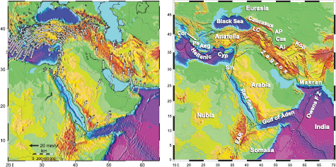
Figure 11. (Left) GPS velocities and 67% (one-sigma) confidence error ellipses relative to the Eurasian plate for the Africa–Arabia–Eurasia continental collision zone. (Right) Tectonic setting. From Reilinger et al (2006). Copyright 2006. This material is reproduced with permission of John Wiley & Sons, Inc.
Download figure:
Standard image High-resolution image
Figure 12. (Top) The 1993–2011 GPS velocity field for the western US relative to the North America plate. Error ellipses are 67% confidence. (Bottom) Close-up of the Cascadia margin. From McCaffrey et al (2013). Copyright 2013. This material is reproduced with permission of John Wiley & Sons, Inc.
Download figure:
Standard image High-resolution image
Figure 13. Velocities at seafloor monuments (blue and red vectors) and on-land reference stations (black vectors) relative to northeast Honshu, Japan (taken to be on the North American plate). The white arrow shows the NUVEL-1A (section 4.3) relative velocity of the subducting Pacific plate; the velocity vectors follow a similar direction with diminishing magnitude towards the western coast showing that the region of deformation from the trench spans about 500 km. The blue and red arrows at seafloor station MYGI show the velocities for the periods from May 2002 to August 2005 and from December 2006 to February 2011, and those at FUKU show the velocities for the periods from July 2002 to February 2011 and from July 2002 to March 2008, respectively, indicating spatiotemporal variations in interplate coupling. The error ellipses are 67% confidence. From Sato et al (2013). Copyright 2013. This material is reproduced with permission of John Wiley & Sons, Inc.
Download figure:
Standard image High-resolution image4.5.3. Fault slip models.
In the simplest model of a single plate boundary fault, near-fault interseismic GPS velocities provide information about strain accumulation. Translating surface displacements and velocities from a network of GPS stations spanning a fault zone into fault slip rates at depth is model dependent, and requires numerous physical assumptions, such as crustal rheology, fault depth, and degree of coupling (aseismic creep versus a locked fault). In line with elastic rebound theory (section 4.2), a simple and remarkably apt model to describe surface deformation is a dislocation in an elastic half-space (Chinnery 1961, Savage and Burford 1973). A model of a dislocation surface of horizontal length 2L, vertical width W, and dip δ embedded in an infinite elastic half-space with the top of the fault depth h below the free surface was applied to 3D surface displacements for three large earthquakes in the western US and Alaska (Savage and Hastie 1966). The following formulation (Savage and Burford 1973) has been used extensively to model interseismic deformation in a transform fault ('strike-slip') environment by an infinitely long locked vertical strike-slip fault in a homogeneous elastic half-space as
where  is the interseismic slip rate at infinite distance along the fault,
  is the orthogonal distance from the fault, and D is the fault's locking depth. The fault parallel velocity profile is time independent. The assumption is that the fault is locked to depth D, beneath which the fault zone creeps at a steady slip rate equal to the relative plate velocity. This is the simplest case of a block model where two infinite elastic blocks are locked at their boundary and accumulating strain, decreasing as a function of the orthogonal distance away from the fault. The strain is fully released during an earthquake (coseismically). However, we know from observations that strain accumulation is the not the inverse of the coseismic strain release, but has a broader spatial extent (figure 14). Furthermore, the presence of postseismic deformation (section 4.6) indicates a viscoelastic response in the lithosphere. This was examined for thrust faulting at the Japan subduction zone for both an elastic crust and an elastic lithosphere over a viscoelastic asthenosphere (Savage 1983). In another study in a strike-slip environment (Savage and Lisowski 1998) an elastic model was fit to trilateration data along the 'big bend', the 300 km curving segment of the San Andreas fault, but a discrepancy was observed between the model locking depth of 25 km compared to a 10–15 km depth from seismicity and laboratory rock mechanics experiments. This discrepancy led the authors to invoke a viscous relaxation model to explain the data. This model presumes that the steady-state motion driven by background plate tectonic loading is perturbed by sudden stress changes after a large earthquake. This has been explained by variations on two basic mechanisms: deep fault aseismic afterslip in the lower crust (below the brittle seismogenic layer) (Fitch and Scholz 1971) (this is further discussed in section 4.8.2 on transient deformation) and viscoelastic relaxation of the lower crust or upper mantle (Nur and Mavko 1974, Savage 1983). It was shown, however, that surface deformation for a long strike-slip fault could be modeled equivalently as an elastic plate (upper crust) overlying a viscoelastic half-space (lower crust and mantle, the 2-layer model in figure 14) or by a vertical fault embedded in an elastic half-space with variable slip along the fault plane (Savage and Prescott 1978, Savage 1990, Fay and Humphreys 2005).
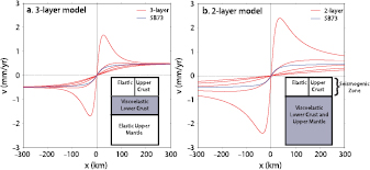
Figure 14. (a) Time-variable fault-parallel velocity profiles for a three-layer model with a 20 km thick elastic upper crust and a 20 km thick viscoelastic lower crust with a viscosity of 1019 Pa · s overlying an elastic upper mantle. (b) Time-variable fault-parallel velocity profiles for the two-layer model with a 20 km thick upper crust overlying the viscoelastic lower crust and upper mantle with a viscosity of 1019 Pa · s. The time-dependent velocity profiles are shown at different stages of the earthquake cycle. The line with largest curvature denotes the velocities as a function of distance from the fault in the period immediately after an earthquake (early in the earthquake cycle), where the effects of postseismic deformation are significant. The other three red lines are later and later in the earthquake cycle until the velocities closely follow the steady state. The recurrence interval is assumed to be 300 years. The vertical line in the elastic upper crust denotes the fault with a depth of 20 km. Time-independent interseismic velocity profiles from the (single-layer) steady elastic half-space model (67) (Savage and Burford 1973) (SB73) are shown by the blue line. Adapted from DeVries and Meade (2013). Copyright 2013. This material is reproduced with permission of John Wiley & Sons, Inc.
Download figure:
Standard image High-resolution imageFor steady-state slip during interseismic and coseismic (section 4.7) deformation, analytic solutions for surface deformation due to shear and tensile faults in a half-space for point and finite (rectangular) sources in an isotropic and elastic medium (1-layer model) are still extensively used for modeling static finite-fault slip (Okada 1985). They begin with the displacement field  for the dislocation
  across a surface
  (e.g. a fault plane) given by
Here  is the Kronecker delta,
  and
and  are Lamé's elastic constants that specify the elastic medium, and
  is the direction cosine of the normal to the surface element
  according to the Einstein summation convention. The term
  is the ith component of the surface displacement at (
 due to the jth direction point force of magnitude F at (
 ) on the fault plane. The
  -axis is taken along strike and the elastic medium occupies the region z ⩽ 0;
  ,
,  ,
,  are elementary dislocations defined to correspond to shear (strike slip), dip slip, and tensile components, respectively, for arbitrary dislocation (figure 15). Analytic solutions for (68) are provided for surface displacement, strain, and tilt observations in strike-slip, thrust, and normal fault environments, and for point source and rectangular finite fault source models of length L and width W (figure 15) (Okada 1985). The Okada formulation has been extensively used to model coseismic, interseismic, and volcanic deformation, and was expanded to include the analytical solution for deformation in the interior of the half-space (Okada 1992). Furthermore, the formulations are given for scenarios that are dependent or independent of the elastic media. Crustal deformation studies often assume a linear isotropic elastic medium where
  =
=  . This is a Poisson solid with a Poisson's ratio of 1/4, which is consistent with values of 0.23–0.28 estimated from P and S wave velocities in the upper crust (Dziewonski and Anderson 1981). Significant improvements are made by modeling deformation in a layered half-space, which brings the modeling into better consistency with the modeling of seismic waves. Additional improvements can be seen from considering the 3D structure of the Earth's interior through finite element modeling or similar techniques. The reader is referred to a useful summary in the documentation of computer algorithms for Okada's formulation (Feigl and Dupré 1999).
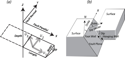
Figure 15. Fault slip geometry (a) Coordinate system at the surface and at depth along the fault plane. Slip vectors U1, U2, U3 represent dislocations of hanging wall with respect to the foot wall signed such that a positive U1 is a left-lateral strike slip, a positive U2 is a thrusting dip slip, and U3 is a tensile slip, in this case for a reverse fault. Adapted from Okada 1985. Copyright 1985 Seismological Society of America. (b) Description of fault slip nomenclature, in this case a normal fault. Adapted with permission from Gabi Laske.
Download figure:
Standard image High-resolution image4.5.4. Plate boundary deformation models.
Here we extend the discussion from a single fault to multiple faults and complex plate boundary zones, sampled with GPS velocity vectors (figures 11–13, table 1) and other geodetic data. A logical extension, in terms of the distributed deformation end member (section 4.4) and the simple elastic model of a dislocation in a half-space (Savage and Burford 1973) described in the previous section, is a model of rotating rigid elastic blocks ('microplates') (McCaffrey 2002) each with its own Euler vector, with the provision for interseismic strain accumulation. As an example, a lithospheric block model for the southwestern US was developed from a large database of GPS velocities, seismic and geologic data, consisting of finite faults defining 23 rigid elastic blocks (McCaffrey 2005). In this model, fault traces are consistent within a spherical cap representation, most faults are vertical, and their down dip extent is constrained to be within the seismogenic zone. For this region, 20 km is taken as the average depth of microseismicity, below which the lithosphere is assumed to be moving at the relative plate velocity. Provision is made for interseismic coupling, that is, differentiating between locked and creeping faults with a normalized parameter that varies between zero (full creep) and one (full locking). A similar approach was used to develop a detailed block model for the Cascadia subduction zone (McCaffrey et al 2013) (figure 12).
Another block model of crustal deformation that includes the effects of block rotation and interseismic strain accumulation was developed for the mostly strike-slip environment of southern California based on GPS velocities at 840 stations with observations over about a ten year period ending in 2001 (Meade and Hager 2005). It also includes a spherical cap formulation with the option of a dip slip fault component (a deviation from a strictly vertical strike-slip fault). We now review the details of their model. First, they invoke the equivalency of a model for a long strike-slip fault as an elastic upper crust overlying a viscoelastic half-space (lower crust and mantle) or by a vertical fault embedded in an elastic half-space with variable slip and locking depth along the fault plane (Savage 1990). As shown in figure 14 (2-layer model), in the immediate aftermath of an earthquake the near-fault velocities are relatively high and correspond to an elastic model as fast slip rates and shallow locking depths. Conversely, late in the earthquake cycle, the lower near-fault velocities correspond to slower slip rates and deeper locking depths, more closely resembling the simpler (1-layer) elastic model. This is equivalent to assuming high viscosity in the viscoelastic model, or that the southern California crust is well into (>40%) the earthquake cycle (figure 14). Then, assuming linear elasticity, the interseismic velocity  can be expressed as the difference between the block velocity
  and the yearly 'coseismic slip deficit' (CSD) velocity
  such that,

This means that as the crust is further into the earthquake cycle, the CSD diminishes until coseismic rupture occurs. The CSD velocity is a function of the GPS coordinate vector  , and the fault geometry represented by
  . Block models on a spherical cap may be calculated with a flat Earth assumption. When employing Okada's (1985) elastic solution (68), the error incurred by this 'flattening' will be less than 1%. However, when including far-field displacements as data input to the block model it may be advisable to retain the spherical geometry. Then, ignoring any fault normal motion, the 3D GPS velocity of an arbitrary location on a block can be represented by the vector product of the angular velocity (Euler) vector
  and the GPS position

where  represents a cross product that is a function of the GPS station coordinate vector
  . Okada's (1985) analytical solutions for surface displacement due to a buried dislocation in a half-space can then be used to determine the CSD term. Because far field velocities are used and Okada's (1985) solutions are for a flat Earth, a local oblique Mercator projection is applied to each fault in the block model such that the slip deficit velocity is

where  is the fault slip rate vector,
  is the rotation matrix in a local north, east, and up system (37),
  is the projection matrix for the station and fault positions from spherical coordinates onto the planar geometry, and
  contains Okada's (1985) analytic solutions that relate slip on the faults to motions at the surface (Green's function; Farrell, 1972). The fault slip rates are then

where  projects the rotation vectors onto a relative velocity at the middle of the fault and
  projects the relative velocity onto the fault plane. The previous three equations can be combined and substituted into the first (69) to express the interseismic velocities in terms of a single multiplication of the angular velocity vector

where  is the combination of the rotation matrices in equations (71) and (72). The inverse problem for the block motions,
 , can now be formulated from these equations as
The left-hand side represents the data used in the inversion, the GPS interseismic velocities  , a priori slip rates
  from geological constraints and a priori block motions
  (Okada 1985). These can each receive different weights depending on their known or perceived reliability. The system (74) in the form of (15) is then inverted by weighted least squares (19). This study (Meade and Hager 2005) found significant variations in slip rates long the San Andreas fault with 5 mm/yr in the San Bernardino segment and up to 36 mm yr−1 on the Carrizo segment. They also echoed conclusions (McCaffrey 2005) that it is difficult to decipher rheological properties of the crust and mantle from this approach, but noted a lack of evidence for postseismic motion and concluded that this most likely means the crust and uppermost mantle have high viscosities in this region. This is in opposition to other investigations (Hearn et al 2013) that found that the discrepancy between geologic and geodetic slip rates from block models could potentially be explained by long-lived postseismic processes in the presence of a weak asthenosphere.
In another example of a distributed crustal deformation model, velocities at 731 GPS sites and nine Holocene–Late Quaternary geologic fault slip rates were inverted to estimate micro-plate rotation rates, interseismic elastic strain accumulation, fault slip rates on major structures, and strain rates within 24 tectonic micro-plates inferred from active fault maps in the greater Tibetan Plateau region at the India–Asia collision zone (Loveless and Meade 2011). They determined that 85% of deformation could be explained by localization of slip on major faults, with the remaining 15% accommodated by internal processes at the sub-block scale, suggesting that forces applied to tectonic micro-plates drive fault system activity over decadal to Quaternary time scales in this region. In another study, a 2-layer and 3-layer viscoelastic model (figure 14) was applied to geodetic observations before and after two large earthquakes on the Tibetan Plateau to estimate the viscosity of the crust below a 20 km thick seismogenic layer (DeVries and Meade 2013). They found a weak (viscosity ⩽1018.5 Pa · s) and thin (⩽20 km) midcrustal layer (3-layer model, figure 14) that explains observations of both near-fault strain localization late in the earthquake cycle and rapid (>50 mm yr−1) postseismic velocities.
GPS velocities have been extensively used for the longest studied and most intensely instrumented plate boundary is the San Andreas fault (SAF) system in California, a complicated mostly, but not exclusively, transform system consisting of multiple faults on land and offshore. The last major earthquake on the San Andreas fault was the 1906 Mw 7.9–8.0 San Francisco earthquake (Thatcher 1975, Ellsworth et al 1981); the central portion of the SAF last ruptured during the 1857 Mw 7.9 Fort Tejon earthquake (Zielke et al 2010). The long recurrence time (Sieh 1978), combined with the dearth of a large rupture on the southernmost portion of the fault, suggest that the southern segment represents the highest hazard in the fault system (Fialko 2006). In the last 30 years GPS surveys have sampled the SAF system (SAFS) and over a thousand cGPS stations are now operating throughout the region. The horizontal velocities and their uncertainties in terms of 2D error ellipses given by the Southern California Earthquake Center (SCEC) Crustal Motion Model version 3 (Shen et al 2011) was developed in part to reconcile derived geodetic slip rates and published geologic slip rates (primarily determined by geomorphology and paleoseismology (Rockwell and Ben Zion 2007)). A problem common to these types of studies and noted earlier (McCaffrey 2005, Meade and Hager 2005) is that the GPS record is still not long enough to span a complete earthquake cycle and GPS velocities in the various tectonic blocks are possibly sampling at different times within that cycle, i.e. during a period of postseismic deformation. This is a potential explanation for the observed discrepancies between geologic and block-model derived fault slip rates (Meade and Hager 2005, McCaffrey 2005), with geologic slip-rates representing longer-term average behavior. A study attempting to reconcile geologic and geodetic fault-slip discrepancies in southern California used a 3D viscoelastic model of the crustal deformation cycle. It postulated steady-state rotating crustal blocks in an elastic medium separated by locked and/or creeping faults (Wdowinski 2009) overlying a linear 2-layer viscoelastic medium. Time-dependent deformation is attributed to nonsteady interseismic fault creep in the lower crust and viscous flow in the upper mantle (figure 14), and perturbed by periodic earthquakes (Chuang and Johnson 2011).
A comprehensive study (Tong et al 2014) used an earthquake cycle model with a 3D fault geometry within an elastic plate over a viscoelastic half-space (2-layer model) to reconcile geological and geodetic slip rates, to within their uncertainties, on the SAFS. We present a detailed description of this study to illustrate the factors that need to be considered, rather than claiming that it presents a definitive reconciliation of geological and geodetic slip rates. In this model, the multiple fault segments have episodic slip to fault locking depths based on the historical earthquake record and geologic recurrence intervals, with steady slip from the base of the locked zone to the base of the elastic plate (Smith and Sandwell 2004). The model assumes a linear rheology of the viscous layer. According to the viscoelastic model, the observed geodetic velocities should be less than the long-term plate velocity since, as mentioned previously, postseismic effects from past large events can be long-lived; the surface strain rates will increase after a large earthquake and gradually dissipate with a long relaxation time. Each of the 41 fault segments uses a simple fault geometry (Smith-Konter and Sandwell 2009), which is assumed to have uniform slip rate, slip depth, and earthquake history. The locking depths for each segment are based on microseismicity and surface GPS observations (Smith-Konter et al 2011). As part of the 3D model, each fault segment is further divided along nodes into curved 5 km patches. The study is particularly data rich, including more than 2000 horizontal GPS velocities from 1996–2010 and about 54 000 satellite line of site velocities from a combination of InSAR interferograms from Japanese ALOS L-band radar data collected from 2006 to 2011. The GPS velocities are transformed into observations into a reference frame tied to the stable part of the North America plate through its Euler vector (Wdowinski et al 2007), which is used to tie the relative InSAR data into this frame well outside of the study area. GPS site velocities are the key data used in this analysis. The InSAR data, with their higher spatial resolution, are primarily useful for resolving aseismic fault creep (locking depth of zero) along the creeping section of the SAF and the faults along the northern segments of the SAF. Similar approaches that combine GPS velocities and InSAR observations have been employed for the San Andreas and Hayward faults (Lohman and McGuire 2007, Evans et al 2012) in an attempt to define slip rates and differentiate locked from creeping sections of the fault system. Data from locations exhibiting anthropogenic effects on deformation or subsidence (e.g. aquifer recharge, hydrothermal power plants; section 8.2) are typically excluded. These areas are quite extensive in water-challenged California, in particular in the greater Los Angeles region (King et al 2006), the Mojave Desert (Galloway et al 1998), and in the greater San Francisco Bay Area (Schmidt and Bürgmann 2003), as verified from InSAR and GPS observations. During the period of the study (Tong et al 2014) many of the fault segments on the SAFS were late in their interseismic period, so the effects of postseismic deformation were minimal. However, the GPS crustal motion model used in the study ignored postseismic deformation from several southern California events, in particular, the 1992 Mw 7.3 Landers and the 1999 Mw 7.1 Hector Mine earthquakes (Shen et al 2011). Furthermore, the velocity field did not include GPS displacements after the 4 April 2010 Mw 7.2 El Mayor-Cucapah, Mexico earthquake that caused significant coseismic and postseismic deformation over most of southern California (Gonzalez-Ortega et al 2014). To account for the neglected postseismic deformation, it was reintroduced into the GPS velocity vectors based on a slip model (Fialko 2004a) estimated to be on the order of 1.5 mm yr−1. Likewise, possible long-term postseismic effects from the 1857 Mw 7.9 Fort Tejon and 1906 Mw 7.9 San Francisco earthquakes were introduced into the earthquake cycle model. Unlike most previous investigations, historical earthquakes and recurrence intervals from the year 1000 to the present (Smith and Sandwell 2006) were tightly integrated. The study finds that a basic 2-layer viscoelastic model (a thick elastic plate overlying a viscoelastic half-space used in many earlier studies, figure 14) is preferable over the 1-layer elastic half-space model; applying the elastic model results in a 10 mm yr−1 reduction in slip rates compared to the geological model (Tong et al 2014). To reconcile the geodetic and geologic slip rates it is also necessary to add a dip slip component to some of the 41 SAFS fault segments, rather than assume a simple vertical strike-slip fault. Furthermore, the assumed rheological properties of the viscoelastic layer are critical; they found the preferred viscosity is 1019 Pa · s with a 60 km thick elastic plate; 16 GPS cross-fault transects along the length of the San Andreas fault generally favored the thick elastic layer except for the three segments characterized by aseismic creep. In a related study (Wdowinski et al 2007) velocity time series were analyzed from 840 sites along the San Andreas Fault with a similar viscoelastic framework to find that most of the data could be explained by elastic strain accumulation and viscoelastic relaxation in the upper mantle. They also found that the largest model residuals (the difference between model and observation) concentrated around the San Andreas fault in the Mojave block and suggested that this might be a result of crustal strength variations across the fault not being properly accounted for. It was found (Hearn et al 2013) that if the asthenospheric viscosity is low then the postseismic effects from past earthquakes can be long-lived and significantly affect the modeling of the GPS velocity vectors under the elastic assumption. A more focused study on slip partitioning (Lindsey and Fialko 2013) in southern California concluded that the assumed fault geometry and fault dip can explain observed asymmetric strain partitioning (Fialko 2006) and help reconcile geodetic and geologic slip rates, while moderate elastic heterogeneities in the crust seen in seismic tomography studies were not deemed a significant factor.
4.5.5. Interseismic strain segmentation.
Interseismic strain segmentation indicates spatial variability in interseismic coupling, defined as the degree of locking of a fault during the period of stress build-up between seismic events (McCaffrey 1996). It is clear that this is important in hazard assessment because it is an indicator of whether slip in a region may be occurring aseismically and, hence, have relatively lower hazard. The 26 December 2004 Mw 9.3 Sumatra–Andaman earthquake (Ammon et al 2005, Banerjee et al 2005, Ishii et al 2005, Lay et al 2005, Stein and Okal 2005, Subarya et al 2006, Chlieh et al 2007), followed by the Mw 8.7 Nias-Simeulue earthquake of 28 March 2005 (Briggs et al 2006) is a good example of strain segmentation, since the two earthquakes ruptured adjacent segments of the Sumatra subduction zone (figure 16). The 2004 event generated a devastating tsunami resulting in over 250 000 casualties, the majority of them on the nearby Sumatra mainland, with inundation heights of up to 30 m (Paris et al 2007). The region had experienced two consecutive tsunamis in 1344 ± 3 C.E. and 1394 ± 2 C.E. (Sieh et al 2015). Previous geodetic studies of interseismic deformation in this region indicated that the pattern of strain accumulation on the Sumatra subduction zone between 0.5°S and 2°N was significantly different from that south of 0.5°S. This apparent spatial variation in the interseismic velocity field coincided with the separation between the rupture zones of previous great earthquakes that occurred on the Sumatra subduction zone in 1833 and 1861 (Newcomb and McCann 1987). The rupture boundary appeared as an abrupt change in the trench-normal strain accumulation rate (as inferred from the trench-normal GPS velocities). The Nias-Simeulue earthquake occurred in approximately the same region that broke in 1861 a 300 km long segment directly SE of and abutting the 2004 Mw 9.3 Sumatra–Andaman rupture zone (Subarya et al 2006). The Mentawai segment of the megathrust (0.5°S–5°S) that produced M > 8 earthquakes in 1797 and 1833 remained fully locked and flanked by two regions of low coupling, the Batu Islands to the NW and Enggano Island to the SE. The 12 September 2007 Mentawai earthquake sequence (Mw 8.5 and Mw 7.9) only partially ruptured the 1833 rupture zone (Konca et al 2008, Sieh et al 2008), and the 25 October 2010 Mw 7.8 Mentawai earthquake ruptured the same segment but was shallow, an updip of the 2007 ruptures, causing a tsunami that took 509 lives (Yue et al 2014). GPS velocities from GPS measurements in the period 1991–2001 prior to the sequence of large events on the Sumatra megathrust starting with the 2004 Mw 9.3 Sumatra–Andaman event showed partial to full coupling on two segments, which then appeared to be slipping freely based on GPS velocities from data collected through to 2007 (figure 16) (Prawirodirdjo et al 2010).
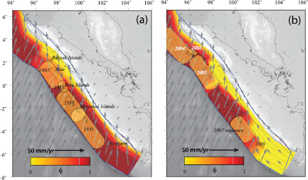
Figure 16. (a) Modeled interseismic velocity field (gray arrows) of the Sumatra subduction zone for the period leading up to 21st century. Shading on the fore arc represents the value of the coupling coefficient  used in the interseismic model (
 = 0 denotes creep,
  = 1 denotes fully locked). The yellow patches show estimated rupture zones of significant subduction earthquakes prior to the 20th century. (b) Modeled velocity field circa 2005–7 (gray arrows). The shading on the forearc represents coupling coefficient values. The yellow patches show rupture zones of subduction earthquakes in the first decade of the 21st century. From Prawirodirdjo et al (2010). Copyright 2010. This material is reproduced with permission of John Wiley & Sons, Inc.
Download figure:
Standard image High-resolution imageSpatial variations in interseismic coupling have been observed at other subduction zones with large historical earthquakes, e.g. Alaska (Freymueller et al 2008), Japan (Ozawa et al 2002, 2007, Hashimoto et al 2009, Liu et al 2010a) and South America (Moreno et al 2008). The spatial variations in coupling in Japan are anti-correlated with areas of repeating small seismic events in aseismically slipping zones (Igarashi et al 2003). The deviations from a simple model of large coseismic slip release correlated with accumulated slip deficit noted in Chile (Moreno et al 2010) and Japan (Ozawa et al 2011) indicate there is more research to be done in using slip deficit as a predictive tool for the timing, magnitude, and spatial extent of future earthquakes. The degree of interseismic coupling may vary in time as well as space; identifying temporal changes may be important in establishing the initial stress state on the fault surface. Studies are focusing on simulations of fully dynamic numerical models, e.g. to test the dependence of earthquake rupture patterns and interseismic coupling on spatial variations in fault friction (Kaneko et al 2010).
With the relatively short historical record (~30 years) of GPS observations it is not simple to separate spatial changes in interseismic strain (and inferred coupling) at different fault segments from possible temporal changes due to the postseismic deformation on segments at different stages of the earthquake cycle (see section 4.6 and the 2- and 3-layer models in figure 14). The studies referenced above using GPS observations along the Sumatra megathrust late in the earthquake cycle and, presumably, the GPS velocities reflected the steady interseismic rate.
4.5.6. Velocity and strain rate fields.
Given a series of point velocities over a zone of deformation, it is useful to create a velocity field model that can be interpolated to any location within the region. Such a model, and the topic of this section, can then be used to produce a strain rate map for the region, which is useful for assessing seismic hazards. Another application is the datum problem for land surveyors working across plate boundaries. Using a velocity field model derived from displacement time series (section 3.2) and an underlying fault slip model (section 4.5.4), one can relate surveys performed at any epoch to a 'fixed' datum defined at a particular epoch of time to provide geodetic control for mapmaking and geographic information systems (GISs) (Pearson et al 2010). Likewise, the true-of-date coordinates of any GPS station can be computed for various applications, such as providing input station coordinates at the onset of an earthquake or defining epoch date coordinates as the definition of a geodetic datum in regions of active crustal deformation.
A regional velocity field and a corresponding strain-rate field are derived from a finite number of point velocity vectors estimated from geodetic observations (GPS, InSAR). The strain rate field can be derived as the gradient of the velocity field. The accumulated strain field is derived by integration over a time interval of interest. The GPS-derived velocity vectors are computed with respect to the 'absolute' terrestrial reference frame (ITRF), as described in section 2.5.3, but for focused plate boundary studies they are transformed into a frame most appropriate for the region of interest. For example, the reference frame for a study of the Cascadia subduction zone may be the rotation pole of the North America plate (figure 12), or for the study of a single fault the vectors may be transformed into fault parallel and fault normal components.
A velocity field and a corresponding strain rate field can be produced in at least two ways. Using a distributed block model of deformation described in the previous section (McCaffrey 2005, Meade and Hager 2005), a velocity field can be derived as a forward problem with the input of fault geometry slip rates and depths (the same approach used to generate a coseismic field was shown in figure 5). The second approach applies the continuum model of crustal deformation (section 4.4), and requires an interpolation function and a constraint on fault slip rates within a region of interest. Neither approach (distributed or continuum) is unique or objective. They are dependent on the distribution and number of geodetic observing stations and other data sources, the choice of model parameters, and the assumed noise characteristics of the observations and model. One could ask whether a continuum mechanics approach usually applied on the micro level in a rock mechanics laboratory, for example, is applicable to a series of point displacement measurements on the Earth's crust. In any case, these are several theoretical spatial and temporal assumptions that must be met: That the material (the Earth's crust) is continuous, the material can be subdivided into infinitesimal elements and retain the same properties throughout, and that the deformation (strain) is infinitesimal and instantaneous. The first two criteria are met by the assumption of elasticity and the third by GPS strain being small at any instant in time and instantaneous compared to the geological rate of deformation. Indeed the last assumption is still a matter of speculation, that is, whether the rate of GPS displacement is equal to the geological rate. These assumptions are intended for the interseismic period and are violated during an earthquake when discontinuities occur in the medium and in the postseismic period when the background strain is disturbed.
It may be that the elastic strain at plate boundaries perhaps modeled with block rotations is the most interesting in terms of assessing seismic hazard, rather than the strain-rate field, per se. Nevertheless, constructing velocity and strain-rate fields is still the subject of active research as the quantity and quality of GPS and other geodetic data increase. Furthermore, while the average velocity field is of widespread interest, the identification of transients (section 4.8) or departures from the secular trend over a region is also important.
4.5.6.1. Regional strain-rate fields.
The horizontal velocity field on the Earth's surface can be expressed as

where  is the radial vector,
  is the radial unit vector of direction cosines of each point on the Earth's surface, and
  is a 3D rotation vector function. To invert for strain rates (e.g. by weighted least squares) from the observed spatially-averaged strain rate tensor components (e.g. obtained from Quaternary fault slip rates), a mathematical function must be chosen to describe
  ; one such function is bicubic Bessel interpolation on a curvilinear grid (Haines and Holt 1993). The inversion minimizes the following function
where subscripts ij, pq denote the tensor components of the strain rate tensor,  is the a priori variance–covariance matrix of the average horizontal strain rate tensor in each grid area, n is the total number of grid areas,
  is the a priori variance–covariance matrix of the observed velocity vectors, and m is the total number of observed velocities. The advantage of this spherical approach is that it allows coverage over a large area. In one study the model velocity and strain-rate field were inverted using point velocities from cGPS, sGPS, and very long baseline interferometry (VLBI) at the western US Pacific and North America transform plate boundary zone (Shen-tu et al 1999). In another study constraints were applied on the style and direction of model strain rates from earthquake centroid moment tensor catalogs (section 5.1) within the plate boundary zones in eastern Indonesia and the Philippines, and from sGPS measurements at the Australian and Pacific plate boundary in New Zealand (Beavan and Haines 2001).
It is common practice to analyze just the horizontal velocities to infer the details of deformation/strain over the region spanned by the network. A 2D approach is justified in a focused region; in any case the vertical component is not as precise as the horizontal and including it may contaminate the resulting strain rate field. An equally spaced grid is designed for the region (e.g. a Delauney triangulation) and each velocity is weighted as a function of the distance d of the station to the center of its grid (e.g. triangle), for example using a Gaussian weighted scheme,
where  is a constant that specifies the downweighting with station distance; it behaves as the standard deviation of a normal distribution. Once the velocity field model is created, one can proceed to develop a strain rate model. The following 2D formulation (Shen et al 1996, Allmendinger et al 2007) uses the Gaussian weighting scheme for homogeneous deformation. The observed GPS velocity u at a given point i is expressed as
where  is the 2D position vector of the station in the final state, ti is a translation (the displacement with respect to the origin of reference frame), Lij is the velocity gradient tensor, and Δxj is the displacement between the station and the grid point. The velocity gradient tensor can be decomposed into a symmetric and anti-symmetric component such that
Here E is the strain rate tensor, Ω is the rotation rate tensor, and  are the components of the velocity gradient tensor
  . The elements of the velocity gradient tensor can be estimated through an inverse problem using the linear model
where G is the design matrix (the Green's functions). The parameter vector l contains the velocity gradient and translation terms ((79) and (80)), and n is the number of GPS stations. The vector l can be solved through linear least squares

where P is the Gaussian weighting factor (77). The estimated shear strain rate is defined as the off-diagonal term of the strain rate tensor (79)
and the principal components of the strain rate are
The estimated maximum shear strain rate is given by the difference between the principal strain rates,

The dilatation rate, δ, is simply the trace of the strain rate tensor

The dilatation rate serves as a proxy for extension in two dimensions (in three dimensions, dilatation is the volumetric change). The rotation rate, ω, comes from the rotation rate tensor and is defined as
where positive values of ω correspond to counterclockwise rotations.
Regional strain and rotation rates were inverted from observed GPS velocities to calculate the full 2D velocity gradient tensor and determine the physical parameters, such as the principal shortening and extension rate axes, the vertical axis of rotation, and two-dimensional (2D) volume strain, for three continental plateaus (Allmendinger et al 2007). They found that these parameters are very consistent with long-term geological features over relatively large areas for collisional plateaus in Tibet, Anatolia (figure 17) and a subduction-related plateau in the central Andes (the Altiplano). The GPS velocity fields were used to define a uniformly-spaced grid over each region using distance weighting interpolation (77). This approach was also applied to the study of deformation over smaller regions in the greater Los Angeles basin (Shen et al 1996) and the Imperial Valley, southern California (Crowell et al 2013). These types of models are used for calculating strain accumulation for seismic hazard assessment, by noting areas that display relatively large strain rates.

Figure 17. Map of GPS strain and rotation rates for the eastern Mediterranean and Middle East. The principal tectonic structures are denoted by heavy back lines. The principal infinitesimal horizontal strain axes are denoted with short colored line segments scaled by the absolute value of their magnitude with red indicating extension and blue shortening. The colors show the variation in magnitude of rotation about a vertical, downward axis, with red indicating clockwise rotation and blue counterclockwise. The black box denotes the region affected by the 1999 Mw 7.5 Izmit earthquake. From Allmendinger et al (2007). Copyright 2007. This material is reproduced with permission of John Wiley & Sons, Inc.
Download figure:
Standard image High-resolution image4.5.6.2. Global strain rate fields.
The widespread installation of cGPS sites at both plate boundaries and plate interiors and sGPS observations at plate boundaries, has allowed the compilation of global strain rate maps. In one study (Kreemer et al 2014), global plate motions and plate boundary deformation were modeled in a unified manner by a global velocity gradient tensor field using station velocity data from GPS and other space geodetic methods, Quaternary fault slip rates, and seismic moment tensor information (section 5.2.1) for shallow earthquakes (figure 18). They defined broad regions of deformation along plate boundaries and other areas known to violate the rigidity assumption of plate tectonics; about 14% of the Earth was allowed to deform in this model. These results can be utilized for hazard assessment to identify regions of high strain rate, although the resolution is coarse. There are interesting features in the global strain rates; strain rates are highest at oceanic transforms and spreading centers. The strain rate at subduction zones is variable, but generally high and there are broad zones of diffuse deformation in the continental interiors affected by subduction and convergence, such as the North America plate and the Eurasian plate, where shortening across the Himalayas is clearly discernible. Areas where GPS coverage has improved over the last decade such as in Iran and Italy show a very rich pattern of deformation that was not previously resolvable. These results can be utilized to identify regions of high strain such as the area of the 25 April, 2015 Mw 7.8 Gorkha, Nepal earthquake.
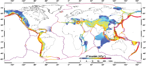
Figure 18. Global strain rate model. Contours are of the second invariant of the strain rate field. The color scale is not linear and is saturated at high values. The white areas were assumed to be rigid plates and no strain rates were calculated there. Instead, the rigid body rotation of these plates was imposed as a boundary condition when solving for plate boundary strain rates from the geodetic velocities. The black box denotes the region of the 2015 Mw 7.8 Nepal earthquake. Adapted from Kreemer et al (2014). Copyright 2014. This material is reproduced with permission of John Wiley & Sons, Inc.
Download figure:
Standard image High-resolution imageAssuming that long-term seismic moment release rates are proportional to the geodetically determined deformation the global patterns of strain have hazard implications. The strain rates can be converted to expected geodetic moment accumulation rates, which can be used to forecast expected shallow seismicity rates (Bird and Kreemer 2014). This procedure has a large uncertainty because a thickness for the seismogenic zone and an amount of coupling at the plate interface must be assumed. Both of these quantities are poorly known at many plate boundaries, but the approach has promise. Furthermore, global computations of strain at plate boundaries can provide further constraints on the behavior of the mantle. Global dynamic models were used to quantify the importance of lateral viscosity variations in the lithosphere and asthenosphere on both surface motions and stresses within the plates and plate boundary zones; it was found that there is significant complexity in this dependence (Ghosh and Holt 2012) (figure 19). Knowledge of the surface strain field has been used to constrain the bulk properties and kinematic behavior of the crust and mantle (Yoshida 2010, Husson 2012) and to correlate with a number of other geophysical observations, mainly from global seismology (Zhu and Tromp 2003).
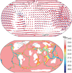
Figure 19. (Top). Kinematic no-net rotation-rate MORVEL (figure 9) model (MORVEL—blue arrows), compared to a global dynamic model in a no-net-rotation frame (red arrows). The dynamic model includes contributions from both coupling with whole mantle convection and lithosphere structure and topography (Bottom). The corresponding best-fitting absolute viscosity model (top 100 km). From Ghosh and Holt (2012), copyright 2012. Reproduced with permission from AAAS.
Download figure:
Standard image High-resolution image4.6. Postseismic deformation
Postseismic deformation refers to the decay usually discernible for extended periods after a medium or greater earthquake when the crust and uppermost mantle return to their steady deformation rate. Postseismic motion seen in GPS displacement time series are often parametrically fit with either an exponential or logarithmic function consisting of an amplitude and a decay time (figure 8), or some combination thereof (section 3.2). A more physical approach is to model the postseismic motion through one or more physical mechanisms in order to distinguish between different rheological models (Takeuchi and Fialko 2013), to infer the state of stress in the crust, and to gain insight into seismic hazards. One of the first significant opportunities to study coseismic and postseismic deformation with cGPS and sGPS was the 1992 Mw 7.3 Landers earthquake California, which caused significant coseismic deformation throughout southern California (Hudnut et al 1994, Pollitz et al 2000, Fialko 2004a, Fialko 2004b). This earthquake also demonstrated the value of the new InSAR technique with a spectacular view of the coseismic (Massonnet et al 1993) and postseismic (Massonnet et al 1996) deformation fields. A study within a year of the event showed that the postseismic deformation released the equivalent of about 15% of the seismic moment of the mainshock (Shen et al 1994). Another study using data collected by cGPS surveys along a transect of stations established across the rupture zone showed 100 mm of right-lateral and 50 mm of fault-normal postseismic displacement in the 3.4 year interval after the event attributed to right-lateral slip in the depth interval 10–30 km on the downward extension of the rupture trace (Savage and Svarc 1997). Later studies investigated several possible physical processes with GPS and complementary InSAR measurements: Poroelastic rebound (Peltzer et al 1998), viscoelastic relaxation of the lower crust and upper mantle (Pollitz et al 1998, Deng et al 1998), and a combination of poroelastic relaxation above the brittle-ductile transition in the crust/upper mantle and localized shear deformation on and below the Landers rupture with significant pore fluids and interconnected pore space throughout the seismogenic layer to a depth of 15 km or greater (Fialko 2004a). A more recent study of early (five months) postseismic deformation after the 2010 Mw 7.2 El Mayor-Cucapah, Mexico earthquake using near-field GPS and InSAR observations was explained by a combination of afterslip, fault zone contraction, and a possible minor contribution of poroelastic rebound, while the far-field data required, most likely, viscoelastic relaxation in the ductile substrate (Gonzalez-Ortega et al 2014). Larger-scale postseismic processes need to consider faults within the tectonic engine and the loading cycle and include variations on two basic processes: Deep fault aseismic afterslip in the lower crust (below the brittle seismogenic layer; this is discussed further in section 4.8.2) and viscoelastic relaxation in the lower crust or upper mantle introduced earlier in section 4.5.3 (figure 14). Smaller-scale near-fault processes may consider the fault as more of an isolated system, and include poroelastic rebound, fault zone contraction, and stress-driven slip on the fault through rate and state friction models.
4.6.1. Larger-scale processes.
The model of viscous relaxation for explaining postseismic deformation presumes that the steady-state motion driven by background plate tectonic loading is perturbed by sudden stress changes after a large earthquake, which includes a viscoelastic relaxation of the lower crust and upper mantle (figure 14) (Pollitz et al 2001). For example, vertical strike-slip faults have been modeled as 3D planar dislocations within the elastic upper crust overlying a stratified viscoelastic plastosphere (Pollitz et al 2015), areas that deform elastically over short time-scales but undergo viscous stress relaxation over longer time-scales, in contrast to the schizosphere, which refers to the portion of the upper crust that deforms elastically during interseismic periods (Scholz 2002, Hilley et al 2005) (figure 14). During an earthquake, the fault planes accommodate shear dislocations followed by a postseismic period, when the plastosphere relaxes with the faults locked until the next earthquake. The stress evolution at a particular point is dependent on the viscosity of the lithosphere and may vary from linear (long relaxation time) to highly non-linear (short relaxation time). Non-linearity assumes that the mean earthquake recurrence interval on a particular fault is shorter than the relaxation time of the plastosphere. The stress evolution in the San Francisco Bay region since the 1838 San Francisco Peninsular earthquake was inferred using a catalog of historical earthquakes, geodetic data, seismic data, and model parameters of the viscoelastic coupling model of strain accumulation constrained by GPS data (Pollitz et al 2015).
The postseismic deformation seen in horizontal GPS displacement time series after the 1992 Mw 7.3 Landers earthquake and three years after the 1999 Mw 7.1 Hector Mine earthquake in the Mojave Desert, California indicated that a power law model of viscous flow in the upper mantle fit the data significantly better than linear stress–strain rate (Newtonian) models (Freed and Bürgmann 2004). The basic relationship for a power-law rheology is given by

where  is the strain rate,
  is the differential stress (coseismic stress change),
  is the power-law exponent, Q is the activation energy, R is the universal gas constant, T is the temperature, and A is a scale factor. It reduces to the Newtonian model when n = 1. The corresponding effective viscosity is given by
A power-law model with n = 3.5 provided the best fit, implying that viscosity varies spatially with stress causing localization of strain, and varies temporally as the stress evolves (Freed and Bürgmann 2004). It is interesting to note that the model did not fit the vertical GPS displacements, implying that other postseismic processes may also be occurring, such as fault-zone collapse and poroelastic rebound, but this could also be due to the lesser precision in the observations. In fault zone collapse following large events a fault-perpendicular shortening is observed in the geodetic measurements (Massonnet et al 1996, Gonzalez-Ortega et al 2014). As an appropriate transition to the next section, it has been hypothesized that this is due to the closure of dilatant cracks and the ejection of fluids following coseismic rupture. In poroelastic rebound there is pore-fluid flow in the host rock due to induced pore pressure changes. This produces measurable deformation and has been observed following large events (Rousset et al 2012).
4.6.2. Smaller-scale processes.
Laboratory friction experiments have been extensively performed to determine the constitutive relationships between shear and normal stress and friction for a variety of rocks. Since earthquakes nucleate on geological faults, and assuming that empirical laboratory results can be applied to the geologic fault process, it is important to understand the frictional force resisting the relative motion of the rocks that slide past each other, in particular at seismogenic depths. A frictional approach to model fault mechanics assumes that slip occurs on a very narrow (sub-centimeter level) interface between the rock surfaces, which are under extreme pressure (normal stress). Starting with the Mohr-Coulomb failure criterion, the coefficient of friction  can be approximated by amplitude of shear stress
  in the direction of sliding and normal stress
  by
by
(Byerlee 1978) (figure 20). At the lower end of normal stresses (up to 2 Kbars), the coefficient of maximum friction is found in laboratory experiments for a wide range of rock types to be about 0.85 (or equivalently the shear stress required to cause sliding is  = 0.85
 ). For higher stresses up to 20 Kbars, the best linear fit of normal stress against shear stress is
  = 0.5 + 0.6
 These relationships are independent of rock type when the fault interface is finely ground, totally interlocked, or irregular but initially locked. When gouge material or fluids are present, the coefficient of friction is much lower (Byerlee 1978).

Figure 20. Schematic of a unit area of fault slip. In a rate- and state-dependent friction model, the friction stress  is a function of the normal stress
  , the slip rate
  and the surface state variables
  (91).
(91).
Download figure:
Standard image High-resolution imageThe rate- and state-dependent friction framework (Ruina 1983, Dieterich 1979a, 1992, Tse and Rice,1986, Lapusta and Liu 1999, Lapusta et al 2000, Rice et al 2001, Scholz 2002) based on empirical constitutive laws is described in this section on postseismic deformation, although it has been applied to fault behavior for all phases of the earthquake cycle. In this framework (figure 20), localized shear stress  on a fault surface is a function of slip rate
  and a state variable
  (see Ruina (1983) for a discussion of multiple state variables) that represents the evolving properties of the number of contact points between the two irregular surfaces of the fault such that
Here  is the coefficient of friction at the arbitrary reference slip rate
  ,
,  is the evolving slip rate (sliding velocity) on the fault, a and b are the frictional parameters, and
  is a critical (characteristic) slip distance. The term
  of (91a) describes the positive direct velocity effect, and in (92b) the state variable
  represents (negative) velocity effects that evolve over
  (Scholz 2002). That is, a sudden increase in sliding velocity (e.g. in an earthquake) results in an immediate increase in friction with magnitude according to empirical parameter a followed by a decrease in friction according to empirical parameter b, over
  (also determined empirically). The state variable after friction reaches steady state (
 ) is given by
  . It follows from (92a) and where
  is the friction at steady state that
 ![$\partial {{\mu}_{s}}/\partial [\ln s]=\boldsymbol{a}-\boldsymbol{b}$](https://content.cld.iop.org/journals/0034-4885/79/10/106801/revision1/ropaa04ddieqn292.gif) ,
, ![$\frac{\partial \mu}{\partial [\ln s]}{{\mid}_{\theta}}=\boldsymbol{a}$](https://content.cld.iop.org/journals/0034-4885/79/10/106801/revision1/ropaa04ddieqn293.gif) is the direct velocity effect on friction, and
is the direct velocity effect on friction, and  is the evolution of friction over the critical distance following a velocity change (reflecting a fading memory of the old contact state);
  denotes velocity weakening, representing a material that under loading will exhibit unstable stick-slip behavior, while
  indicates velocity strengthening, representing a stable behavior of material that will creep when stress is applied (Scholz 2002).
A rate- and state-dependent friction approach (Barbot et al 2009) was used to model postseismic deformation for the 2004 Mw 6.0 Parkfield, California earthquake using three years of GPS displacements from a network of 14 GPS stations (Langbein and Bock 2004) spanning the San Andreas fault (figure 4), using a modified form of (91a)
Assuming that the coseismic change in normal stress is negligible compared to the background and lithostatic tectonic stress and that the pre-earthquake Coulomb stress ((90) and (95)) is negligible compared to the coseismic stress change, then 'the effective stress' driving afterslip on the fault plane is the shear component of coseismic loading ( ). Then the slip rate is given by
and assuming steady state ( ) results in a rate strengthening (
 ) constitutive law between slip rate and stress

In order to test whether this formulation can explain the three year GPS displacement time series, the reaction of the fault to the coseismic slip for simple shear is given by
where G is the shear modulus, L is the linear dimension of the crack, and C is a constant near unity that is a function of geometry. The rheological parameter G* represents the stiffness of the slip patch. By an inversion process, the optimal time scale  and k values were estimated for each component of the GPS time series (Barbot et al 2009). Regardless of the rheology, the values were nearly identical, so that a single postseismic process could be attributed for the earthquake. The overall postseismic signal was clearly identified as the first mode of a principal component analysis (63)–(66) (figure 21). The best fit of the first mode indicated values of C = 1.25;
  = 4.8, and k = 7. This is consistent with a postseismic afterslip that is 75% complete within 3 years after the earthquake. The best estimate of the frictional parameters was
  = 7 × 10⁻³ (rate strengthening), which is at the high end of laboratory results. The results are also consistent with the majority of afterslip concentrated at 5 km depth, but highly variable along strike, inferring that there are large along strike variations in rate and state frictional properties. An analysis was also performed for a power law model that results from a ductile finite (yet narrow) shear zone at the fault. The comparison indicated that for the analysis of GPS displacement time series after the 2006 Mw 6.0 Parkfield event, the rate and state friction model was preferred. The power law model indicated a longer lasting transient (about six years). This is one example of how GPS displacement time series may be able to distinguish between different postseismic models using an underlying physical process to fit the displacements (94) (Gonzalez-Ortega et al 2014), rather than a parametric fit (logarithmic, exponential; (40) and (41)), as discussed in section 3.2.
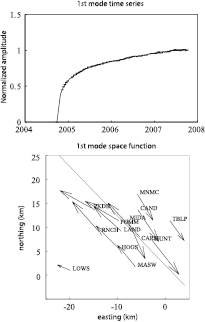
Figure 21. (Top) PCA decomposition of the Parkfield GPS time series (see also figures 4 and 5). The first mode, with 95% of the total variance, corresponds to the postseismic signal. (Bottom) The corresponding GPS displacements exhibit the expected signature of right-lateral slip on the fault and correspond to the cumulated surface displacement due to postseismic deformation after three years. From Barbot et al (2009). Copyright 2009. This material is reproduced with permission of John Wiley & Sons, Inc.
Download figure:
Standard image High-resolution image4.6.3. Stress triggering.
It was suggested that the 1999 Mw 7.1 Hector Mine earthquake was the result of delayed triggering from postseismic loading following the 1992 Mw 7.3 Landers earthquake (Freed and Lin 2001), shown by comparing the Coulomb stress change (King et al 1994b, Stein et al 1997, Stein 1999, Lin and Stein 2004) produced by coseismic and postseismic loading. In this scenario, the Coulomb stress  is defined as

and it represents the stress necessary to drive a fault to failure,  is the ambient shear stress,
  the coefficient of friction,
  the fault-normal stress, and p is the pore pressure. The Coulomb stress is composed of fault-parallel and fault normal components (figure 20). The fault parallel component is the ambient shear stress
  in the along-strike direction. The fault normal component is the sum of the local normal stress and the pore pressure, which can act to clamp or unclamp the fault. Coseismic motions can induce shear-stress changes in the vicinity of rupture that will inhibit or promote failure on optimally oriented faults. Similarly, as seen from (95), an increase in pore pressure will reduce the effective normal stress
  as the pore space attempts to expand, reducing the normal stress on the fault and unclamping it. Coseismic Coulomb stress changes were not significantly high at the site of the Hector Mine earthquake hypocenter, but when postseismic loadings were considered, the stress increase at the hypocenter was as high as 0.1–0.2 MP, leading to a hypothesis that postseismic effects in the period between 1992 and 1999 triggered the Hector Mine event (Freed and Lin 2001).
At shorter time-scales and through methodical analysis of thrust and strike-slip earthquakes it was shown that the aftershock distribution patterns following medium to large events can be explained through Coulomb stress transfer (Lin and Stein 2004). They analyzed the slip distribution patterns of known and historical ruptures and correlated them to the observed distribution of aftershocks and found that the simple mechanism of Coulomb stress transfer could readily explain the observed distributions of aftershocks. Particularly interesting in that study was the analysis of the 1960 Mw 9.5 Valdivia, Chile event. They used a slip distribution determined from geodetic and coastal uplift measurements (Barrientos and Ward 1990) and found that 75% of the aftershocks occurred in regions of Coulomb stress increase. Similarly they found that the 1857 Mw 7.9 Ft. Tejon earthquake on the Southern San Andreas fault in California produced a noticeable Coulomb stress increase in the region of the 1953 Mw 7.2 Kern County earthquake to the north. The Kern county event was a thrust earthquake just north of the San Gorgonio pass, which divides the San Bernardino and Coachella segments of the San Andreas fault. This observation is interesting because it illustrates the complex relationship between faults in active plate boundaries, the stress from rupture on the San Andreas, a right-lateral fault, promoted the failure of a large thrust fault elsewhere in the plate boundary almost 100 years later.
Following the 2011 Tohoku-oki event it was suggested that there had been a 'dynamic overshoot' and that the slip during the event had exceeded the slip deficit accumulated simply from plate tectonic motion (Ide et al 2011). This hypothesis was strengthened by noting that there were hitherto unobserved low-angle normal faulting aftershocks on the megathrust following the event, suggesting that the fault was 'paying back' the overshoot by way of these normal faulting events. Another study looked at the correlation between kinematic slip inversions of the 2011 Mw 9.0 Tohoku-oki earthquake and, not only the geographic distribution of aftershocks, but also their faulting style (Melgar and Bock 2015). They computed the Coulomb stress change of several slip models at the plate interface or 'stress drop' as a result of the earthquake and studied whether areas of positive stress drop (stress relaxation) correlated with the low angle-normal faulting aftershocks, and areas of negative stress drop (stress loading) correlated with thrust aftershocks at the subduction interface. That study found that slip models derived from on-shore GPS and seismic data, which have inherently low resolution (section 5.3, figure 37), showed almost no correlation between the stress drop pattern and the type of aftershocks. However, when offshore tsunami measurements that better resolve shallow slip were jointly inverted with the on-shore GPS and seismic data the correlation increased to modest but positive levels, placing the low-angle normal faulting aftershocks on the areas of largest stress drop (figure 22). All these studies suggest that even in the absence of knowledge about critical parameters such as the pre-event state of stress of the fault or the material properties of the fault itself, if models of the slip distribution during the event can be elaborated that rely on many kinds of geophysical observables, it is still plausible to consider such models as useful for forecasting the type and possible locations of aftershocks.

Figure 22. (a) Stress drop for the kinematic slip inversion (figure 37) using land-based and offshore tsunami data and its correlation with six months of aftershocks occurring within 10 km of the subduction zone slab model and with similar strike and dip. The red circles denote normal faulting aftershocks and the blue crosses thrust faulting aftershocks. The CMT solutions (beach balls) indicate notable aftershocks with a magnitude greater than Mw 6.5. The green star is the hypocenter, and the blue triangles are the on-land stations used in the inversion. The dotted lines are the 10 km depth contours to the slab model (Hayes et al 2012). (b) The same but for the land-only kinematic slip inversion (figure 37). From Melgar and Bock (2015). Copyright 2015. This material is reproduced with permission of John Wiley & Sons, Inc.
Download figure:
Standard image High-resolution image4.6.4. Multiple earthquake cycles.
In practice, it is difficult to separate different postseismic processes from each other and to quantify the relative contributions of each. The availability of extensive GPS data for a growing number of earthquakes has allowed researchers to examine a variety of postseismic models. Nevertheless, this is a complex problem requiring numerous assumptions; for example, estimates of upper mantle viscosity from a variety of sources, including GPS, still differ by up to three orders of magnitude (Bürgmann and Dresen 2008). Estimates of postseismic deformation are important not only for studying crustal and mantle rheology, but for hazards and earthquake triggering.
To summarize the sections on interseismic and postseismic deformation, GPS and InSAR data, whose coverage is increasing both temporally and spatially, are providing important constraints on physically plausible models of the earthquake cycle and starting to reconcile geodetic and geologic fault slip rates. Through dynamic modeling of subduction zone earthquakes with heterogeneous frictional properties, it was argued (Kaneko et al 2010) that creeping patches and locked sections of faults, which can be recognized from the observation of interseismic velocity fields, can be used to assess the long term behavior of fault zones. It is possible to model other physical phenomena at fault zones such as shear-induced temperature variations and pore pressure changes inside the fault zone over many events (Liu and Rice 2007, Noda and Lapusta 2010). A fully dynamic model reproduced fault-zone behavior over several earthquake cycles (Barbot et al 2012). It produced recurring earthquakes, such as in the Parkfield region, which has experienced seven medium-sized earthquakes since 1857 (Bakun et al 2005), the latest being the 2004 event, and provided good fits to the observed postseismic and interseismic velocity fields. By examining GPS displacements from different subduction zones at various stages of the earthquake cycle, there is evidence of a unifying picture emerging in which the deformation is controlled by both the short-term (years) and long-term (decades and centuries) viscous behavior of the mantle (Wang et al 2012).
In spite of many of these advances our understanding of the probability of large earthquakes on a given fault and the state absolute stress in the crust are still poorly understood, indicating an 'extremely complex relationship' between tectonic loading and seismic activity (Fialko 2006).
4.7. Coseismic motion
4.7.1. Displacement measurements.
GPS-derived coseismic displacements are used to image the earthquake source, which provides insight, for example, into mechanical fault properties and the potential interactions among individual faults within fault systems due to the complex relationship between strain and stress (Fialko 2004a). In this section, we cover the use of GPS displacements to model the earthquake source, that is, the propagation, geometry, and extent of rupture, and the energy release within the crust, as a complement to seismic measurements and field surface offset measurements. Additional geodetic observations that image the earthquake source include InSAR, seafloor geodesy (Fujita 2006, Sato et al 2011, Bürgmann and Chadwell 2014), off-shore ocean-surface GPS buoy kinematic displacements (Kawai et al 2013), aircraft lidar surveys (Nissen et al 2012, Brooks et al 2013), and coral reef uplift and subsidence (paleogeodesy, Sieh et al 2008).
A note on nomenclature: During an earthquake 'coseismic' motion consists of a dynamic and a static component; the former will dissipate (elastic waves) while the latter represents permanent ('static') displacement. The dynamic component of coseismic motion is measured most precisely with inertial sensors (seismometers, accelerometers), but can also be measured with GPS (section 5.2.2). The permanent surface displacements are input to inversions for 'static' source models, having no temporal dependence and providing only the total accumulated slip on the fault plane. The full coseismic displacements (dynamic and permanent) are input to inversions for 'kinematic' source models that describe the time evolution of the slip and image the rupture propagation along a faulting surface.
The recovery of coseismic displacements with GPS field surveys (sGPS) after an event is problematic because it involves a quick logistical response, which can be especially difficult in remote regions, and of course requires a record of prior surveys. By the time data are collected, there may have been additional motion from afterslip or other postseismic processes that would cause an overestimate of total slip and, thus, earthquake magnitude. Latency is even more pronounced with satellite-based InSAR measurements, which is dependent on the orbit repeat cycle. Thus, cGPS measurements are ideal for monitoring coseismic surface displacements.
The first cGPS-derived coseismic displacements were measured by a handful of stations during the 1992 Mw 7.3 Landers, southern California earthquake (Bock et al 1993, Blewitt et al 1993). These data were used to estimate a simple elastic half-space fault slip model (67), seismic moment, and earthquake magnitude. A forward calculation of the slip model provided a coseismic surface deformation field throughout the affected region. Furthermore, the GPS displacement time series indicated short-term postseismic motion of about 1 mm d−1. With the proliferation of cGPS networks across plate boundaries, the use of coseismic surface displacements as input to earthquake source inversions has become routine. As an example, the coseismic displacements for the 2011 Mw 9.0 Tohoku-oki, Japan earthquake were upwards of 5 m of horizontal deformation and over 1 m of subsidence at some coastal sites (figure 23). A rapid static slip model based on a retrospective now-time analysis of 1 Hz GPS data from the Japanese GEONET (GNSS Earth Observation Network System, Sagiya et al 2000) was shown to be obtainable within ~3 min of earthquake initiation (the earthquake duration was 2–3 min, Simons et al 2011). The static inversion (Melgar et al 2013a) using only land-based observation showed up to 30 m of slip at depth over a broad area more than 400 km long (figure 24). The addition of off-shore data and using a kinematic model considerably improved the resolution (figure 35).
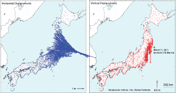
Figure 23. Permanent coseismic displacements due to the 2011 Mw 9.0 Tohoku-oki earthquake, Japan. (Left) Maximum horizontal (blue arrows) and (right) vertical (red arrows). The green star denotes the epicenter. GPS displacement time series were provided by the ARIA team at JPL and Caltech. The GPS raw data were provided to Caltech by the Geospatial Information Authority of Japan. Reproduced with permission from Ron Grapenthin.
Download figure:
Standard image High-resolution image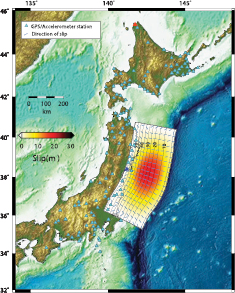
Figure 24. Static slip inversion of the 2011 Tohoku-oki earthquake using a subset of all the available GPS stations. The black contours indicate the depth in kilometers using the 3D fault model of Hayes et al (2011). Reproduced with permission from Melgar et al (2013a). Copyright 2013. This material is reproduced with permission of John Wiley & Sons, Inc.
Download figure:
Standard image High-resolution image4.7.2. General model of the earthquake source.
Now we present a general finite-fault slip model (Minson et al 2013) that can be used for kinematic slip inversions for the earthquake source using GPS and seismic data input. If we ignore temporal dependence, it reduces to the static model. The general 3D kinematic finite-fault slip model for spatio-temporal slip on the fault rupture at depth in an elastic medium can be written as a summation over  sources, in two directions: j = 1 along strike and j = 2 along dip, in three surface directions by


The vector d denotes surface displacements in a local reference frame in the ith direction to receiver location  , either dynamic displacements estimated through the integration of velocity or accelerometer observations and/or by directly-measured geodetic or seismogeodetic displacements (section 5.2.3). The vector
  contains the magnitude of slip in the strike and dip directions (the earthquake slip vector, see figure 14) at the kth subfault. The element
  is the Green's function (Farrell 1972). It contains the expected motions from a unit dislocation in the jth direction at the kth source observed at the ith component of the receiver location
  on the surface of an elastic medium (
 is referred to as the modified Green's function).
  is a source-time function that describes how slip evolves with time at the kth source; it has a duration
  , and
, and  is the time of rupture initiation at this same subfault. The symbol | means 'given'. A complete kinematic description of the earthquake rupture requires the two components of slip (strike slip and dip slip) for the kth source, t0 and Tr for each of the
  unit sources that make up the fault rupture. The time for the onset of rupture at a particular source
  depends on the rupture speed, Vr at which the rupture front is propagating. If no constraints are applied, then the kinematic inversion is an undetermined problem with an infinite number of solutions. Typically, to render it tractable the dislocation surface is discretized into subfaults and a simple parametrization for the source time function is assumed. If the rupture speed and slip duration are considered unknowns, then the inversion is non-linear and the cost-function can be multi-modal. This problem can be solved with Monte Carlo techniques such as simulated annealing, genetic algorithms, and Bayesian inversion. However, if a functional model for d is assumed and an upper bound is placed on rupture speed, then the problem can be linearized by the multi-time window method. Deficiencies in the Green's function resulting from an imperfect elastic Earth structure model introduce artifacts into the solution (Minson et al 2013). Assumed structure models can vary from a homogeneous to a layered 1D model (Dziewonski and Anderson 1981) to a fully heterogeneous 3D model (Kohler et al 2003, Matsubara et al 2008). Also, the parameterization of the source-time function
  can vary from simple isosceles triangles to complex shapes derived from fracture mechanic, as well as assumptions for the rupture velocity Vr ranging from freely varying to fixed. The fault geometry is often pre-defined; for example, the Slab 1.0 model provides a 3D compilation of global and regional subduction-zone geometries (Hayes and Wald 2009, Hayes et al 2009). The reader is referred to a helpful review of kinematic inversion techniques (Ide 2007).
If time dependence is neglected, a simpler problem can be solved. This is known as a static finite fault-slip model (figure 24); a homogeneous elastic half-space (e.g. Okada 1985) or 1D or 3D Green's functions can be used. GPS and other permanent displacements such as subsampled and unwrapped interferograms are the primary source of data. In this case, the model ((96) and (97)) is independent of the time evolution of the seismic source and reduces to
or in matrix form

where  is the vector of the estimated surface displacements and
  is the vector of the source model parameters. Note that the Green's function matrix G serves here as the design matrix, which includes the partial derivatives in the linearization for a weighted least squares inversion (19).
The earthquake source problem, whether kinematic or static, is a non-unique and ill-conditioned problem. This is typically ameliorated through regularization, which requires that some smoothness constraint be satisfied. Once a regularization approach has been selected the traditional and simplest approach is to solve the earthquake source inverse problem through weighted least squares, as was described previously for the GPS data analysis (section 2.3). To arrive at a unique solution for the earthquake source, the observation equations are augmented by smoothing constraints on the fault interface (Crowell et al 2012, Melgar et al 2013a) such that

where T is a smoothness matrix and λ a smoothing parameter. In this formulation, the measurement uncertainties are not subject to any probability distribution; only an assumption on the mean and covariances of observation error  , while the constraints are often assumed without error. Possible choices for the smoothness criteria are Laplacian smoothing, Tikhonov (minimum norm) smoothing, as well as positivity constraints, sparsity constraints, and fault rupture length minimization. Selection of the appropriate level of smoothing can be achieved by assessing the minimum solution norm on the data misfit curve (or 'L curve') required to fit the data. Another approach that does not require knowledge of the complete error description (i.e. errors in the Green's function in addition to observational errors) utilizes Akaike's Bayesian Information Criterion (Akaike 1980, Fukahata 2003). This is a model selection criterion that estimates the loss of information in an inversion as a consequence of regularization and penalizes unnecessary model complexity. These are only marginally related to physical assumptions. One advantage of this method is that it can be automated and applied to near real-time modeling applications (section 5.2). Discretization and regularization are inherently subjective considerations and significantly different earthquake source models have been obtained by different authors for the same event (Ide 2007, Minson et al 2013, figure 25), especially when the data are sparse, or different collections of data are used. This can make interpretation of the underlying source processes difficult, but there are often features that are common to all slip inversions irrespective of the inversion strategy; these can then be considered robust features of the source process.

Figure 25. An illustration of the variability in earthquake source models. Small differences in inversion techniques and data can lead to large differences in inferred earthquake slip models. We show here four published slip models for the 1992 Mw 7.3 Landers, California earthquake (Cohee and Beroza 1994, Wald and Heaton 1994, Cotton and Campillo 1995, Hernandez et al 1999). Reproduced with permission from figure 1 in Minson et al (2013). Copyright 2013. This material is reproduced with permission of John Wiley & Sons, Inc.
Download figure:
Standard image High-resolution imageA promising approach to modeling the earthquake source is a stochastic Bayesian formulation through Monte Carlo Markov Chain formulations (MCMCs), which samples all models that are consistent with observations, while restricting the ensemble to those that fit the assumptions about the underlying physics (Minson et al 2013, Dettmer et al 2014). This may be preferable over inverse methods that use subjective regularization or smoothing (100), which are not strictly based on minimizing a model norm that is based on physical constraints. Although it does not require matrix inversion, it is computationally more burdensome since it involves the calculation of many thousands of forward problems. The Bayesian approach (the following development is from Minson et al 2013) following from the Bayes Theorem is

where  is the vector of static and/or dynamic observations, and
  is the vector of model parameters, where
  refers to the probability density function (PDF).
  is the a priori PDF of the model parameter (its expectation),
  is the PDF of the predicted (expected) observation d given the model
  , and
, and  is the a posteriori PDF. The PDF of the predicted observation vector d is dependent on the measurement errors of
  and the uncertain model prediction errors. In this case, we start out with the same linearized model, but explicitly assume that there are model errors
  as well as measurement errors
  , and that they are normally distributed. It follows that the sum of these errors are normally distributed so that the forward model can then be written as the likelihood function
Where  is an
is an  -dimensional vector of the observed kinematic time series such as seismic velocities or high-rate GPS displacement waveforms,
  is the corresponding output vector of the kinematic forward model (96) and θ is a vector of model parameters.
  is the combined bias of the observation and model errors, and can be assumed to be zero.
  is a covariance matrix for the kinematic problem, which includes the combined uncertainties from the measurement errors and model prediction errors. This expression provides a PDF of the distribution of model errors. The expression
  is a measure of how well the observed measurements
  agree with the forward model (i.e. 'the goodness of fit'). The model errors in the context of a finite fault slip inversion may consist of systematic (non-random) errors in the physical model and/or systematic errors in the observations. The former include any deviation of the physical model from the true nature of the earthquake process or parameterization, e.g. errors in the earthquake's hypocenter estimate, fault geometry, and Earth structure. Systematic errors in observations may be due to, e.g. a mis-modeling (or non-modeling) of atmospheric refraction (section 6.1) on the radio signals or signal multipath (section 8.4) when determining the GPS position. This formulation then assumes that the observation errors have zero mean and covariance
  while the systematic model errors have a different covariance matrix
  and may have a non-zero mean ('bias')
  . Then, the model vector
  in the likelihood function for the kinematic model is composed of both kinematic and static parameters,

while the static model is composed only of static parameters

In practice, it is assumed that that the model errors are unbiased, i.e.  . Then the static problem model likelihood function is
Here  is a covariance matrix for the static problem.
In order to use Bayes formula (101), the a priori model PDF,  for the slip parameters. This could be accomplished by using a finite centroid moment tensor solution from seismogeodesy (Melgar et al 2012) and computing some estimate of its PDF. For the static problem, the solution provides a priori estimates of magnitude, average strike, dip and rake (figure 15), and source extent, and can be obtained without prior assumptions on the fault geometry for rapid finite fault slip inversion. The parameters and their uncertainties can be used to generate the a priori PDFs. Thus, the MCMC approach to static and kinematic inversion starts off with a guess of the possible model; this is then perturbed, and if it fits the data better than the unperturbed model it is accepted with some probability, typically derived from the Metropolis criterion (Sambridge and Mosegaard 2002), and then perturbed again. After many thousands of models are produced, the resulting ensemble can be analyzed to determine which model is most likely and to choose its associated PDF through statistical inference. An example application was presented for a static inversion (Minson et al 2014) with real-time GPS data and also for a kinematic inversion (Dettmer et al 2014).
As noted, coseismic slip inversions are of interest for understanding the physical processes governing the earthquake source. However, they can also lead to insights about the bulk behavior of the crust; for example, a joint inversion of GPS and InSAR data for the 1992 Mw7.3 Landers earthquake (Fialko 2004a) found that the coseismic model, thus derived, was in agreement with seismically derived source models. Notably the crust behaved linearly during the coseismic process. This is an important observation; crustal rocks contain cracks and other imperfections at a variety of length scales. It is possible that as they deform in response to coseismic loading; the partial opening of these cracks leads to an overall bulk reduction of the elastic moduli. That is to say, the elastic moduli would be stress-dependent and no longer linear. Furthermore, it was demonstrated (Fialko 2004a) that at the length scales that can be investigated with GPS and InSAR no such behavior was observed; rather, the asymmetries in the displacement field were attributed strictly to the complex geometry of the faulting surface. This conclusion supports the assumption of linearity that underpins most if not all the coseismic inversions of geodetic data to date. This study also observed a wide area, perhaps as wide as 2 km, around the fault zone with reduced shear modulus. This compliant zone represents a long-lived damage zone surrounding the faulting surface. These damage zones and how they form, evolve, and their implications for source physics, elastic wave propagation, and hazard are now the focus of many geophysical studies (Cochran et al 2009).
4.8. Transient deformation
4.8.1. Motivation.
GPS time series analysis has the first-order goal to extract the signals of tectonic interest, including interseismic, coseismic, and postseismic deformation. Interseismic deformation at plate boundaries by definition is driven by slow steady tectonic motion not exceeding about 280 mm yr−1 (Bevis et al 1995) and is quantified by estimating station velocity from the geodetic time series. However, it is expected that the simple model of the earthquake cycle is at best applicable over the long term, averaged over many earthquakes. Along a particular plate boundary, it may be that strain is segmented in space (Prawirodirdjo et al 1997), and that it may be possible to provide better resolution in terms of variations in the recurrence time of earthquakes than a simple average rate (Sieh et al 2008) (section 4.5.5). Furthermore, slip accompanying earthquakes (coseismic and postseismic deformation) appear to account for only a fraction of plate tectonic displacements (Schwartz and Rokosky 2007). It is this search for an explanation of the next degree of complexity that motivates the search for transient motions. Transients are often characterized by very low slip rates on low strength faults, usually on the order of mm/day to mm/yr, orders of magnitude lower than those during regular earthquakes that can be as high as meters per second, and that can occur immediately following earthquake rupture as well as during the interseismic period. There have been observations that suggest that they might also occur before some large events, but the observations are disputed (Roeloffs 2006). The reader is referred to reviews of these phenomena (Schwartz and Roskosky 2007, Beroza and Ide 2011). Due to their slow slip rates, transients generate little to no appreciable elastic wave energy and cannot be observed with seismic instruments. Rather they are seen as deviations in GPS time series from the interseismic trend. Below we describe three types of transients; afterslip, slow-slip earthquakes, and pre-seismic slip (Lohman and Murray 2013).
4.8.2. Afterslip transients.
Afterslip is slip immediately following an earthquake and on the same faulting surface. It is characterized by slip duration of a few days to a few months, with a rapid initial slip rate followed by logarithmic decay (Schwartz and Roskosky 2007). This is different from postseismic viscoelastic relaxation (section 4.6), which is a viscoelastic process where the entire volume surrounding an earthquake, notably the lower crust and upper mantle, deforms in the months to years following an event. One way that the two processes have been distinguished is in the depth and sense of motion. Afterslip occurs on the coseismic fault surface occurs at seismogenic depths and is hence most evident in near fault stations. Viscoelastic relaxation is presumed to occur in the mantle or ductile lower crust deeper than the fault plane, and is most evident in very long time series at distant stations (Rousset et al 2012, Bruhat et al 2011). Afterslip was first documented in continental strike-slip faults from trilateration after the 1966 Parkfield earthquake (Smith and Wyss 1968) and from the matching of geologic features following the 1987 Superstition Hills earthquake (Williams and Magistrale 1989). However, it is most prominently expressed following large megathrust earthquakes. Significant afterslip was found following the 1995 M8 Colima earthquake in Mexico (Hutton et al 2001). Modeled GPS time series from the 2001 Mw 8.4 Peru earthquake showed that the afterslip was as much as 25% of coseismic slip (Melbourne et al 2002). Significant afterslip was observed following the 2004 Mw 9.3 Sumatra–Andaman earthquake, although the sparseness of the GPS observations made it difficult to locate it precisely (Chlieh et al 2007). For more recent large earthquakes there have been many observations of afterslip. Widespread deep afterslip (figure 26) was observed following the 2010 M8.8 Maule, Chile earthquake (Vigny et al 2011) and variations in GPS time series up to 420 d after the earthquake were interpreted as pulses of afterslip along the megathrust (Bedford et al 2013). Many studies have found significant deep afterslip for the 2011 Mw 9.0 Tohoku-oki earthquake with an equivalent moment magnitude as high as Mw 8.3 (Ozawa et al 2011, Evans and Meade 2012). Most inversions relying on smoothed least squares show some overlap between the coseismic and afterslip regions (Ozawa et al 2012). However, a novel inversion approach that minimizes a norm that measures sparsity and, thus, allows for sharp variations suggests that the afterslip region is distinct from the coseismic one and located down dip (Evans and Meade 2012). The regions where afterslip and transients can generally occur is believed to be delineated by its material properties, which are assumed to be different from those of portions of the fault that sustain normal coseismic rupture. Typically, it has been assumed that a region that can sustain rapid coseismic slip cannot later sustain slow and stable sliding. However, following the 2011 Mw 9.0 Tohoku-oki earthquake, it was found that eight months of GPS observations were inconsistent with this model and that either afterslip had to occur inside regions that typically sustain normal coseismic rupture or afterslip had to exceed the fully relaxed limit (Johnson et al 2012).
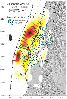
Figure 26. Coseismic and afterslip source model for the 2010 Mw 8.8 Maule, Chile earthquake. The color scale (from 0 to 20 m) shows the extent and the amount of coseismic slip. The arrows depict the amount and direction of slip on the fault plane. The contour lines show the 12 d afterslip (contour level every 10 cm). The dots show the locations and data type used in the inversion (black dots for GPS data; small for survey marks and large for continuous GPS stations; open dots for land-leveling data of natural features or survey marks). The red star shows the hypocenter location and the beach ball is the centroid moment tensor (CMT) solution (section 5.2.1). From Vigny et al (2011), copyright 2011. Reproduced with permission from AAAS.
Download figure:
Standard image High-resolution imageMost of these results have focused on deep afterslip below the mainshock rupture zone, where warm conditions can no longer sustain brittle rock failure. Figure 26 shows an example of this for the 2010 Mw 8.8 Maule earthquake in Chile. The coseismic motions occur mostly seaward off the coast with two main asperities that show up to 20 m of motion. Inversion of the next 12 d of GPS observations reveal up to 0.5 m of afterslip concentrated mostly down dip of the rupture. Intriguingly, the inversion also shows afterslip in the region between the two main rupture patches, suggesting that perhaps the two asperities are separated by a region of velocity strengthening material (section 4.6). If this is the case then this earthquake is an example of a velocity-strengthening barrier separating two asperities (Kaneko et al 2010). However, the same frictional properties that enable afterslip (and inhibit sudden rupture) are present in the shallowest parts of the megathrust, where highly compliant, soft rocks of the shallow subduction zone are found. Shallow afterslip has not been widely observed, likely because GPS sites are all on-shore far away from the shallow megathrust and cannot resolve these motions. An exception is the 1999 Mw 7.5 Chi–Chi Taiwan earthquake, where afterslip was observed throughout the fault depth (Rousset et al 2013). Another example of shallow afterslip was observed from GPS sites on the forearc islands off-shore Sumatra, which were close enough to document shallow afterslip following the 2005 M8.7 Nias earthquake equivalent to an Mw 8.2 event (Hsu et al 2006, Kreemer et al 2006). It is likely that shallow afterslip occurs after many megathrust events, but remains unresolved due to station distribution; offshore tilt and strainmeters and seafloor geodesy (Bürgmann and Chadwell 2014) will do much to shed light on this problem and initial results from seafloor instruments during the 2011 Tohoku-oki earthquake look promising (Sato et al 2011, figures 10 and 13).
4.8.3. Slow slip events.
Another class of transients is referred to as 'slow slip events' (SSEs), although references to 'slow earthquakes' are not uncommon (Linde et al 1996, Ide et al 2007, Ito et al 2007). They have the same mechanism as regular earthquakes but, once again, have very low slip rates. Unlike afterslip, SSEs seem to occur throughout the whole interseismic period. These events were first recognized by modeling anomalies in GPS time series as a slow thrust event in the Bungo Channel in Japan (Hirose et al 1999). Subsequently, a similar event was identified along the Cascadia subduction zone with up to 2 cm of slip at the fault interface that occurred over a period of 1 to 2 weeks (Dragert et al 2001). There, the GPS time series, at the surface, showed a reversal of motion relative to the direction of convergence, with an amplitude of 2–4 mm over an 8–15 d interval in the summer of 1999. These signals were small and only several times larger than the root mean square scatter of the residual time series (0.8 mm in the horizontal components and 3.1 mm in the vertical). The deep slip signal observed with the GPS network (Dragert et al 2001) is consistent with about 20 mm of slip on the slab interface downdip of the seismogenic zone over an area of 50 × 300 km, and equivalent to an earthquake of moment magnitude 6.7. It was subsequently determined that this type of SSE happened with striking regularity at 13–16 month intervals along the subduction zone (Miller et al 2002, Rogers and Dragert 2003, Szeliga et al 2008). Examination of nearly 20 years of GPS time series in Cascadia continues to show the regular occurrence of the SSEs (figure 27). One large SSE was identified in the Guerrero segment of the Mexican subduction zone (Lowry et al 2001, Kostoglodov et al 2003) with many more discovered afterwards and with regular recurrence periods of about four years (Vergnolle et al 2010). SSEs have also been identified in New Zealand (Douglas et al 2005, McCaffrey et al 2008, Wallace and Beavan 2010)), Alaska (Ohta et al 2006) and Costa Rica (Outerbridge et al 2010). In total, six subduction zones have exhibited SSEs (figure 27). However, a systematic description of their geographic distribution remains unknown because many subduction zones have sparse instrumentation.

Figure 27. Detrended 24 year record of daily GPS displacement time series (east component) from GPS station ALBH (48.395°E, 123.490°W) on Vancouver Island, British Columbia indicating, clearly, 18 slow slip events from early 1994 to late 2015. The red line is the parametric fit to the daily time series (section 3.2). The larger scatter in the early 1990s is primarily due to less precise satellite orbits and the limited global GPS infrastructure at that time.
Download figure:
Standard image High-resolution imageFrom what has been observed thus far, some conclusions can be drawn about SSEs. Importantly, they regularly occur with a special kind of seismic event known as tremor. Tremor presents as very long duration seismic signals with no clear wave arrivals, which is now known to be a swarm of many, very small, low-frequency earthquakes (Obara 2002, Obara et al 2004). It is not the purpose of this review to recount the properties of tremor; this can be found summarized elsewhere (Beroza and Ide 2011). However, it should be noted that SSEs are routinely accompanied by tremor and are now considered to be part of the same process. In fact, the combination of the two is often referred to as Episodic Tremor and Slip (ETS). There is variability as to where SSEs occur in a given subduction zone. SSEs in Japan Cascadia and Alaska occur far inland from the trench (up to 200 km, figure 28), while in Mexico and Costa Rica they are much closer to the trench and in the near vicinity of areas known to produce regular megathrust earthquakes. It has long been argued that fluids are a first order control on tremor; however, the distribution of SSEs suggests that the plate rate and the composition and geometry of the slab, which in turn control thermal structure, might be more important for understanding SSEs than fluid migration (Beroza and Ide 2011). The subduction zones where ETS has been observed are all subducting young oceanic crust with ages less than 30 Myrs (figure 28); it is possible that older and colder subduction slabs do not show this behavior. Places with a thermal structure similar to where ETS has been observed thus far such as Ecuador and southern Chile would be likely candidates for further study (Beroza and Ide 2011).

Figure 28. Tremor and slow-slip events (SSEs) in the world's subduction zones. The world map shows colored ocean-floor age plate boundaries (dark blue lines), and six subregions, for which individual detailed maps are shown. The green areas are areas of known SSEs. The purple lines denote rupture areas of known earthquakes and the light blue lines are the isodepth contours of the subducted slab. Reproduced with permission from Beroza and Ide (2011). Copyright 2011 Annual Review of Earth and Planetary Sciences.
Download figure:
Standard image High-resolution imageAlthough the magnitude, timing, and duration of these slow slip events have been well documented, there is still active research on how they are related to stress release over the earthquake cycle, what their implications are for improving probability assessments of large megathrust earthquakes, and whether they are precursors. For example, normal earthquakes grow in size (determined by their seismic moment) as the cube of the rupture duration, and this is taken to be indicative that the stress drop is constant. However, SSE duration scales linearly with moment (Schwartz and Rokosky 2007) suggesting that their relationship to crustal stressing is quite different. It has been pointed out that if the magnitude-duration scaling relationships observed thus far are extended to magnitudes greater than 8, then the slip velocities would be so slow as to never exceed secular plate tectonic rate (Meade and Loveless 2009). Then, a large magnitude SSE would not manifest as the traditional reversal of the velocity field, but rather it would be present as a change in the coupling of the plate interface and only a continuous computation of the coupling coefficient would be able to identify it. SSEs exhibit other interesting characteristics; they seem to be partially modulated by tidal stresses (Hawthorne and Rubin 2010), supporting the notion that they are happening on weak, near critically stressed faults.
Modeling of SSEs and transients associated with slip on faults can be performed much like a coseismic static slip inversion (section 4.7.2). The difference between positions at two epochs is considered an offset and can be used as data in the inversion. A more formal approach is a network inversion Kalman filter that can identify transients related to slip on known faults from geodetic data (Segall and Matthews 1997). The temporal variation of fault slip is estimated non-parametrically by taking slip accelerations to be random Gaussian increments. In this way, fault slip is a sum of steady state and integrated random walk components. At each epoch the Kalman filter estimates the amount of slip on subfaults that make up the entire faulting surface. This approach was used to study the Tokai and Bungo Channel SSEs in Japan in 2000–2 and 2002–4, respectively (Liu et al 2010b). They were able to identify complex slip histories that are not always easy to resolve with the traditional slip inversion approach and concluded that the SSEs slipped in a region bounded by two locked patches of the megathrust and the epicenters of low frequency earthquakes. They further concluded that the long term behavior of these SSEs is likely the controlling variable in low-frequency earthquake activity.
The relationship of SSEs to normal earthquakes has been the subject of significant study as well. As noted in figure 28, where the locations of SSEs and coseismic ruptures are plotted, in some subduction zones SSEs happen down dip of the region where traditional megathrust events are expected based on higher rates of interseismic strain. If SSEs are happening in the transition zone, then they may be delineating the down-dip limit, where the subduction zone can no longer sustain brittle failure. This is particularly useful especially for the Cascadia subduction zone, where the lack of large megathrust earthquakes recorded instrumentally makes this down dip limit difficult to determine (Chapman and Melbourne 2009). However, in other subduction zones such as Mexico, SSEs occur far up dip and at the same depths as regular earthquakes; therefore, their geographic distribution may be indicating along-strike compositional variations. One SSE was observed underneath Oaxaca in Mexico, which was active until the onset of the 2012 Mw 7.4 Ometepec earthquake (Graham et al 2014). Through Coulomb stress calculations (section 4.6), this study demonstrated that it is possible the earthquake was triggered by the SSE. The full extent of the importance of SSEs in the seismic cycle remains an open and intriguing question.
4.8.4. Preseismic slip.
The last and much-debated class of transient deformation is preseismic slip. This phase has been hypothesized for geologic faults based on small variations to a constant friction prior to a slip event that have been seen in laboratory rock experiments (Dieterich 1979b). Transient deformation was reported at one station preceding an Mw 7.6 aftershock to the 2001 Mw8.4 Peru earthquake (Melbourne and Webb 2002). A subsequent study reported ten credible accounts of preseismic geodetic transients and also noted their absence for many more large earthquakes (Roeloffs 2006). Previously in section 4.6.3 we discussed an example of stress triggering of aftershocks through Coulomb stress transfer from a main shock (we suppose that this could be classified as 'preseismic' slip, 'postseismic' slip, or just 'transient' slip).
Another suggestion is that because tremor is associated with ETS (section 4.8.3), tremor observations can also indicate deep slip that cannot be geodetically observed preceding coseismic rupture (Shelly 2009, 2010). There was also a report of two shallow transients before the 2011 Mw 9.0 Tohoku-oki, Japan event that increased shear stress along the plate boundary (Ito et al 2013). Additionally, in the decade preceding the 2011 Tohoku-oki earthquake it was noted that the GPS derived strain field was decreasing; this was interpreted as a decrease in plate coupling due to afterslip from intraplate events (Ozawa et al 2012). However, it has since been suggested that observed accelerations at GPS sites are best explained by a long-lived deep transient (possibly existing prior to 1996) that migrated up dip in the decades before the 2011 Tohoku-oki earthquake (Mavrommatis et al 2014). The authors of this study do not go as far as to infer causality, but it remains a tantalizing possibility that very long-lived transients can modulate very large earthquake ruptures.
4.8.5. Transient signal simulations.
In light of these many kinds of transient deformation phenomena, their important implications for earthquake seismology and the proliferation of GPS networks, there have been efforts to develop automated techniques to detect and characterize transient deformation signals in GPS time series. Notably, the SCEC sponsored the geodetic transient validation exercise (Lohman and Murray 2013). For this exercise, numerous research groups blind tested both synthetically generated and real observations of transient signals contaminated with realistic GPS noise (Agnew 2013) and tested a number of algorithms to automatically detect transient signals. Detection techniques on daily GPS displacement time series included several algorithms: time series analysis to flag statistically significant rate changes over a range of spatial and temporal scales in the presence of colored noise, the fitting of a predetermined number of piecewise linear segments to the data at each site and subsequently identifying spatial and temporal correlations between the segments at surrounding sites, as well as Kalman filtering with spatial basis functions based either on known faults or on smooth functions related to models of the spatial strain field and the significance of its temporal variations (Granat et al 2013, Holt and Shchrebchenko 2013, Ji and Herring 2013). Efforts such as these and continued observation at plate boundaries around the world will help to elucidate the mechanism behind transients and their implications for earthquake physics and seismic hazards.
5. Natural hazard mitigation systems
5.1. Introduction
The last few decades have witnessed a terrible loss of life and economic disruption caused by tsunamigenic earthquakes impacting coastal communities and infrastructure (Kahn 2005). The events of the last decade have been exceptionally severe. The 2004 Mw 9.3 Sumatra–Andaman earthquake (Ammon et al 2005, Ishii et al 2005, Lay et al 2005, Stein and Okal 2005, Subarya et al 2006) resulted in over 250 000 casualties, the majority of them on the nearby Sumatra mainland, from a tsunami with inundation heights of up to 30 m (Paris et al 2009). The Mw 8.8 2010 Maule earthquake in Chile (Lay et al 2010, Delouis et al 2010) resulted in 124 tsunami-related fatalities and wave heights up to 15–30 m in the near-source coast (Fritz et al 2011). The 2011 Mw 9.0 Tohoku-oki earthquake in Japan (Simons et al 2011, Lay and Kanamori 2011) generated a tsunami with inundation heights as high as 40 m resulting in 18 000 casualties (Mimura et al 2011, Mori et al 2012). The hardest hit in all these three events were those closest to the earthquake source, a scenario for which there exists no adequate early warning system. These are other events (in particular extreme weather and flash flooding, as discussed in section 6 in the context of GPS meteorology) have motivated the proliferation of real-time cGPS geodetic networks that sample at high rates, from 1–10 Hz or greater as the backbone for natural hazard mitigation systems for earthquakes, tsunamis, and volcanic eruptions.
In this section, we begin with rapid models of the earthquake source based on the observed permanent (static) coseismic displacements, followed by GPS observations of the dynamic component of coseismic motion ('GPS seismology') and their use in earthquake rapid response. Then we introduce an optimal combination of real-time high-rate GPS observations and accelerometer data ('seismogeodesy') that yields both coeismic (static and dynamic) displacements and seismic velocity waveforms (seismograms) for the purpose of earthquake early warning and tsunami prediction. Finally, we overview the contributions of the GPS to understanding of magmatic processes and to mitigation systems for volcanic eruption hazards. A word on nomenclature for this section: 'Real-time' refers to the first few seconds to a minute or two after the onset of the earthquake, during which a warning of imminent seismic shaking is possible. 'Now-time' refers to the later period, when rapid response to an emergency is still effective, e.g. based on a rapid model of the earthquake source immediately after dynamic motion has dissipated (2–3 min for large earthquakes) or a tsunami prediction well before the first waves impinge on nearby coastal regions (~15–30 min).
5.2. Earthquakes
5.2.1. Rapid models of the earthquake source.
Inverting GPS-derived coseismic displacements to produce static and kinematic earthquake source models (section 4.7) improves our understanding of the mechanical properties of faults and dynamic Earth processes that underlie the earthquake cycle. It is now commonplace to use both static displacements from cGPS and sGPS, near-field strong-motion acceleration waveforms, and other geodetic data (InSAR) for earthquake source inversion, but after a significant length of time has elapsed since the event occurred (in 'post-processing' rather than in now-time). Some examples with heterogeneous data include the 2003 Mw 6.6 San Simeon (Ji et al 2004, Rolandone et al 2006) and 2004 Mw 6.0 Parkfield (Kim and Dreger 2008) earthquakes in central California, and the Mw 6.6 2005 West Off Fukuoka prefecture earthquake in Japan (Kobayashi et al 2006). The combination of near-source geodetic and seismic strong-motion (accelerometer) data covers a broad spectrum of coseismic motion, from high frequencies (100–200 Hz) to long periods through to the permanent displacement.
Real-time GPS observations open the possibility of estimating now-time slip models of the earthquake source to support rapid response to destructive earthquakes. Rapid determination of the coseismic field as a forward solution to source model inversion (section 4.7.2) contributes to seismic intensity maps over the affected region (Wald 1999) and to tsunami modeling and prediction (section 5.3). It has been demonstrated that realistic static source models can be estimated from GPS coseismic displacements as soon as dynamic shaking has dissipated, usually within a few minutes for the largest events. Using the static displacement field, it is possible to produce source inversion models that range from point source (Melgar et al 2012) to line source moment tensors (Melgar et al 2013a), followed by heterogeneous static slip inversions (Crowell et al 2012, Melgar et al 2013a, Minson et al 2014). As demonstrated for the 2011 Mw 9.0 Tohoku-oki earthquake by a retrospective replay of high rate GPS data collected during the event by the Japanese nation-wide GPS network (Sagiya et al 2000), it would have been possible to obtain a reliable magnitude (Wright et al 2012) and produce a static finite-fault slip model within 2–3 min of earthquake origin time, strictly from the land-based GPS static displacements (Melgar et al 2013a). This information could then have been used (section 5.3) to estimate the uplift of the seafloor as input to reliable tsunami prediction models of extent, inundation, and run-up, well before the first tsunami waves arrived at the coastline (Melgar and Bock 2013). As a first step to now-time static source inversion, it is important to rapidly determine the rupture mechanism (e.g. thrust versus strike-slip) and its basic parameters. This can be obtained through a centroid moment tensor (CMT) solution, which we now describe in some detail as it begins to highlight the complementarity of the GPS to traditional seismic methods for rapid earthquake and tsunami response, particularly in near earthquake source regions where losses of life and property are often the most severe.
A compact representation of the source mechanism of an earthquake is provided by the six independent elements of a symmetric moment tensor (Jost and Herrmann 1989). A complete description also includes the 3D location (centroid) and time of occurrence of the earthquake. The full representation of the seismic source requires ten parameters and is termed the centroid moment tensor (CMT) solution (Backus and Mulcahy 1976, Dziewonski et al 1981, 1983). The CMT is a point-source approximation for a fault rupture of finite extent that can be longer than 1000 km for great earthquakes. Each component of the moment tensor represents a force couple within an elastic medium. For pure shear dislocation, only one pair of orthogonal force couples (a 'double couple') is necessary to describe the source. The non-double couple component of the moment tensor solution represents deviations from the shear-slip assumption due to data noise, violation of the point-source assumption, unknown Earth structure, or source processes not modeled by this approximation such as off-plane faulting. The geographic location of the moment tensor is the point of average moment release (centroid) and differs from the earthquake hypocenter (the point of initiation of rupture). Pictographically, the moment tensor solution is represented by shading with different colors or patterns denoting the compressional and extensional quadrants of motion on a lower hemisphere stereographic projection. These are colloquially known as 'beach balls' and are a way to distinguish between different faulting types (normal, strike-slip or thrust) (e.g. figure 26, which indicates a thrust mechanism). The computation of point-source CMT solutions using long-period teleseismic waveforms ('teleseisms', earthquakes that occur more than ~1000 km from a seismic station) is now standard seismological practice. For example, the Global CMT Project (Ekström et al 2012) produces rapid CMT solutions of earthquakes greater than M5.5 and refined solutions of earthquakes with M > 5 after a several month delay. The GCMT also maintains an archive of historical CMT solutions for more than 25 000 earthquakes.
CMT solutions are used for tectonic studies to determine the stress regime within a region. These are usually limited to medium or smaller-sized earthquakes because of the point source approximation. For larger events, the point source approximation is invalid, even at teleseismic distances. For example, the point-source approximation resulted in a significant underestimate of magnitude of the 2004 Mw 9.3 Great Sumatra, Indonesia earthquake. The GCMT solution estimated a magnitude of Mw 9.0, partially due to the fact that the source region of the earthquake was over 1200 km long and the source duration was close to 10 min (Park et al 2005). That CMT solutions underestimate the full seismic moment release was pointed out in earlier studies, e.g. the 1989 M 8.2 Macquarie Ridge earthquake (Kedar et al 1994). One approach to account for fault finiteness is to perform the CMT analysis at global scales for multiple point sources to mimic a propagating slip pulse (e.g. Tsai et al 2005). Indeed, inversion with 5 point sources leads to a moment magnitude for the Sumatra earthquake of Mw 9.3. Another approach is to study ultra-long period data to assess excitation of the normal modes of the Earth (Stein and Okal 2005).
Rapid computation of a CMT solution is also extremely useful to decision makers and emergency first responders for rapid earthquake response. The moment tensor indicates not only the size (magnitude) of an earthquake, but also the style of faulting and possible orientation of the fault plane. Efforts to improve the speed of CMT solutions by using teleseismic broadband data closer to the source makes use of a long-period phase between the direct seismic P and S waves, called the 'W phase' (Kanamori 2003, Kanamori and Rivera 2008), which stays on scale longer than large amplitude surface waves. The USGS, Pacific Tsunami Warning Center (PTWC) and Institut du Physique du Globe de Strasbourg (IPGP-EOST) routinely calculate rapid CMT solutions using the W phase (Hayes et al 2009). Following the 2011 Mw 9.0 Tohoku-oki earthquake, it was shown that it was feasible to use data at distances as small as 11° (~1200 km) from the source and there are indications that, had regional data been available in real-time, broadband recordings as close as 7° might have been useful as well (Duputel et al 2011). Performing the inversion with data at regional distances (a few hundred km from the source) is difficult because the computations rely on long period data from high-gain seismic sensors (broadband seismometers), which can mechanically clip during strong shaking.
For the 2011 Mw 9.0 Tohoku-oki earthquake it took PTWC 20 min after the origin time to arrive at the first CMT solutions (Hayes et al 2011). The final CMT solution was obtained by the Japanese National Earthquake Information Center (NEIC) 90 min after the origin time using data up to 90° from the rupture. The first estimate of moment magnitude was obtained in about 3 min by the Japan Meteorological Agency (JMA), but was severely underestimated at Mw 6.8 (Hoshiba and Ozaki 2014). Thus, W phase-based inversion schemes, while very robust, require long period displacement records (e.g. 200–1000 s for the 2011 Tohoku-oki event, Duputel et al 2011), and are unusable close to the source in now time. Unlike broadband seismometers, accelerometers do not clip in the near source region. However, it is difficult to extract in real-time long-period motions from strong-motion accelerometer data because of possible instrumental tilts and rotations (Boore and Bommer 2005, Melgar et al 2013b). One approach uses an automated scanning algorithm to calculate CMT solutions from regional long-period (100–200 s) strong-motion (accelerometer) observations (Guilhem et al 2013). The algorithm determined accurate source parameters including the moment magnitude and mechanism of the 2011 Tohoku-oki earthquake within 8 min of its origin time, which is a significant improvement over teleseismic methods, and could be suitable for tsunami warning.
Near-source high-rate GPS data can be used to produce accurate CMT solutions for large earthquakes, which do not rely on teleseismic observations (O'Toole et al 2012, Melgar et al 2013a). The source parameter vector  can be written (O'Toole et al 2012) as

The linearized mathematical model is

where  is the observation vector,
  are the observations,
  is the Green's function matrix (section 4.7.2) relating the change in a source parameter to a surface observation point (station), and the M components
  in spherical coordinates (
 ,
,  ,
,  ) are elements of the moment tensor matrix at the earthquake centroid at time
  .
.
Because the GPS directly provides estimates of displacements, it provides very-long-period information (down to zero frequency, the permanent/static motion), which can be obtained closer to the source. Valid CMT solutions for two moderate magnitude earthquakes in Japan were estimated, the 2005 Mw 6.6 Fukuoka and 2009 Mw 6.9 Iwate-Miyagi earthquakes with GPS data collected as close as 25 km from their source (O'Toole et al 2012). GPS displacements were used to estimate accurate CMT solutions within about 2 min from the GPS static displacements for two large earthquakes, the 2003 Mw 8.3 Tokachi-oki, Japan and the 2010 Mw 7.2 El Mayor-Cucapah, Mexico earthquakes (Crowell et al 2012). The advantages are clear in terms of more rapid earthquake response and tsunami warning (section 5.3), and providing a priori constraints on full finite fault slip modeling (section 4.7.2). Furthermore, the GPS solution only requires an initial starting value for the earthquake location (which is iterated to locate the centroid) and the choice of an elastic Earth model (O'Toole et al 2012).
The point-source approximation for regional CMT calculations with high-rate GPS data is inappropriate for great earthquakes, as documented for the 2011 Mw 9.0 Tohoku-oki event, where the magnitude was underestimated and the centroid poorly located (Melgar et al 2013a). It was shown for a series of great historical earthquakes that analysis of near-source static GPS displacement vectors at stations along the coast parallel to a subduction zone interface could be used to rapidly calculate fault dimensions and average slip, useful for tsunami forecasts (Singh et al 2012) or at global GPS tracking stations (Blewitt et al 2009). The finiteness of the fault can be accommodated by superposition of linear point sources and a grid search for the optimum line azimuth and spatial location (Melgar et al 2013a). A single CMT solution is then obtained by weighted averaging of the individual moment tensors over the line source based on their moment and place the average moment tensor at the location of mean moment release. No a priori information on the fault geometry is required. For the 2011 Mw 9.0 Tohoku-oki earthquake with a magnitude of 9.0, and an average strike, dip, and rake of 204°, 30°, and 95° respectively, were obtained with a source extent of 340 km along strike, which agreed well with the final global CMT solution obtained from teleseismic data (Melgar et al 2013a). This was quickly followed (within seconds) with a realistic finite fault slip inversion. This method requires extracting the permanent displacement from the full displacement waveform (see the next section on GPS seismology). Some approaches to do this include trailing variances (Melgar et al 2013a), a short-term average long-term average (STA/LTA) algorithm analogous to what is used for P wave detection in seismology (Ohta et al 2012), and an exponential weighted moving average (Minson et al 2014). These approaches produce different static estimates as the earthquake unfolds but all converge to the same result. For the 2011 Tohoku-oki event, 1 Hz data from the extensive real-time Japanese GPS network (GEONET, Sagiya 2004) were replayed in simulated now-time mode (Melgar et al 2013a); permanent displacements were obtained at 157 s after rupture initiation and the extended CMT solution within several s after that, quickly followed by a static finite-fault slip inversion for the earthquake source (the inversion can be done efficiently since static deformation modeling has no temporal dependence and the Green's functions (section 4.7.2) need only be computed once at inversion nodes in a pre-defined grid with a database of fault geometries, for example, a 3D fault model of global subduction zones (Hayes et al 2012)). The GPS approach demonstrated a marked improvements over the W phase CMT inversions for this event (Hayes et al 2011). As a comparison, the ShakeMap (Wald et al 1999) and Prompt Assessment of Global Earthquakes for Response (PAGER, Jaiswal et al 2007) products provided by the US Geological Survey were initially released for the affected areas based on point sources. The alerts were later updated to a finite fault source after 2 h and 42 min, significantly extending the length of affected coastline (Hayes et al 2011). The resulting source extent of 340 km derived from the extended CMT approach using GPS data was sufficiently close to the final extent and orientation of slip to be useful for rapid earthquake response and tsunami warning.
Changing paradigms in geophysical inversion are also producing interesting advances in rapid source analysis with GPS data, including a probabilistic approach to moment tensor inversion that relies on neural networks (Kaufl et al 2014) and an algorithm to determine a simplified static slip model using Bayesian inversion (Minson et al 2014). It is noteworthy in the latter study that they inverted simultaneously for the fault model as well as the location and orientation of the dislocation surfaces. The probabilistic approach (section 4.7.2) is becoming commonplace in geophysical inversion because it circumvents problems of regularization and smoothing (often considered unphysical restrictions) in traditional least squares inversion. It requires, however, the selection of suitable prior distributions and relies on the computation of several thousand forward models, making it a computationally intensive approach.
5.2.2. GPS seismology.
GPS observations can also be used to estimate dynamic displacements (Bock et al 2000, Langbein and Bock 2004, Genrich and Bock 2006, Larson et al 2009), as well as static displacements. Real-time GPS data at a rate of one sample per second (1 Hz) or greater by regional networks (distances up to several hundred km) have been recorded for the 1999 Mw 7.1 Hector Mine, California earthquake (Nikolaidis et al 2001; this study used data sampled at 30 s but was the first to demonstrate this capability), near-fault data for the 2003 Mw 6.6 San Simeon, California (Ji et al 2004), the 2003 Mw 8.3 Tokachi-oki, Japan (Miyazaki et al 2004, Emore et al 2007, Crowell et al 2009, 2012), the 2004 Mw 6.0 Parkfield, California (Langbein et al 2005), the 2005 Mw 7.0 West Off Fukuoka Prefecture, Japan (Kobayashi 2006), the 2010 Mw 7.2 El Mayor-Cucapah, Mexico (Crowell et al 2012, Grapenthin et al 2014), and the 2011 Mw 9.0 Tohoku-oki, Japan (Melgar et al 2013a) earthquakes. However, unlike seismic instruments, single-epoch high-rate GPS-estimated displacements are not precise enough to detect smaller seismic phases (P waves) even at near-fault distances. An optimal combination of data from collocated GPS and accelerometer instruments preserves the advantages of both types of observations (seismogeodesy, section 5.2.3).
High-rate GPS networks have also been used to track weak motion, large amplitude teleseismic (Love and Rayleigh) waves from the 2002 Mw 7.9 Denali fault, Alaska earthquake with stations up to 4000 km from the source (Larson et al 2003, Kouba 2003, Bock et al 2004), 14 000 km from the epicenter of the 2004 Mw 9.3 Sumatra–Andaman earthquake (Davis and Smalley 2007), and several thousand km for the 2011 Mw 9.0 Tohoku-oki earthquake (Grapenthin and Freymueller 2011). However, at teleseismic distances dynamic GPS displacements are only accurate enough to measure large earthquakes (~M > 7.5), while traditional seismic measurements at any location can resolve earthquakes as small as M 5.3, a factor of 1000 less than geodesy. On the other hand, many global broadband seismometers clipped during the 2004 Mw 9.3 Sumatra–Andaman earthquake (Park et al 2005).
GPS geodesy and seismology have developed as two disparate disciplines. Initially, GPS geodesy focused on quantifying permanent (aseismic) deformation of the Earth's crust from the global scale (e.g. plate tectonic motion) to the local scale (e.g. single-fault studies, volcanic deformation, subsidence), as well as measuring transient motions deviating from the simple model of a crustal deformation cycle (section 4). Seismology relies on the measurement of dynamic transient ground motions (elastic waves) resulting from seismic sources, including earthquakes, tsunamis, volcanoes, atmospheric and oceanic sources, nuclear explosions, and artificial explosions to study global to local processes. Some applications include studies of the Earth's structure through internal propagation of elastic waves, crustal deformation, natural hazard mitigation, mineral exploration, engineering seismology, and nuclear weapons test monitoring for nonproliferation efforts.
Both geodesy and seismology maintain extensive global infrastructure of monitoring stations and often rely on the temporary field deployment of instruments. Seismic sensors include high-gain ('weak-motion') seismometers that record small amplitude signals and are usually qualified by their bandwidth of sensitivity as broadband or short period. Here, the movement of a test mass inside an electro-mechanical system is proportional to ground velocity. In contrast, low-gain or strong-motion sensors directly measure strong-motion ground acceleration and are often simply called accelerometers. The distinction between high- and low-gain instruments is necessary because the dynamic range of signals in seismology spans many orders of magnitude and no one sensor can measure them all. For large amplitude signals such as during strong shaking, high-gain instruments clip as the motion of the test mass exceeds its mechanical range of motion. Considerations for deploying a GPS and seismic instruments also vary; for example, observatory grade seismometers are ideally located in stable underground seismic vaults or in boreholes to minimize temperature and pressure-induced tilts, and are shielded from electromagnetic interference. Meanwhile, GPS stations are located above ground to view the GPS satellites and avoid significant obstructions (e.g. trees, buildings, mountains). Furthermore, by their focus on a wide range of seismic frequencies, seismic stations generally sample at very high rates (e.g. 100–200 Hz) compared to the GPS, which had been sampled until the last few years at lower rates (15–30 s); this is changing, and cGPS stations are sampling at 1–10 Hz, with some receivers capable of observing at higher rates.
Seismic observations are local with respect to an inertial reference frame. Although the GPS antenna needs to be aligned with the local vertical and gravity field (section 2.3.2), GPS instruments provide spatial (non-inertial) observations with respect to a global terrestrial reference frame (section 2.5.3). Considering their history of development, as well as the different siting requirements for seismometers and GPS instruments, it is not surprising that there have been very few station collocations; this situation is slowly changing as cGPS stations are being upgraded with seismic sensors (accelerometers) because GPS and seismic measurements are complementary. Together, they span the broadest possible frequency range of surface displacements (dynamic and static) (figure 29). Assuming no instrument drift or tilt, a typical broadband seismometer is many orders of magnitude more sensitive, in terms of displacement, than a GPS instrument. Therefore, a GPS is not suitable for far-field response to moderate earthquakes or smaller. GPS noise levels, however, are sufficiently low to resolve most of the surface wave spectrum of moderate events at near-source range and large events at teleseismic distances (see the list of references at the start of this section). At low frequencies (above 1 Hz), GPS noise levels roughly agree with the upper limit of the dynamic range of broadband seismic sensors (figure 29). Since the dynamic range of GPS sensors has no upper limit, GPS and broadband seismic sensors cover together the entire possible range of seismic surface displacement. For higher frequencies, sensitivities of both sensors do not overlap (figure 29). Compared to a GPS that directly measures displacements, seismic sensor-derived displacements are obtained by a single integration of observed broadband velocities or a double integration of observed accelerations; velocity measurements are preferred, since the conversion to displacement waveforms requires one less integration. Due to the dynamic range limits of seismometers, the accuracy of absolute displacements thus derived is poor. Likewise, doubly integrating accelerations to displacements is problematic and results in unphysical velocity and displacements, which at long periods grow unbounded as time progresses across a range of temporal and spatial scales (Melgar et al 2013b). Sources of error include numerical error in the integration procedure, mechanical hysteresis, cross-axis sensitivity between the test mass/electromechanical system used to measure each component of motion and, most commonly, unresolved rotational motions (Graizer 1979, Iwan et al 1985, Boore 2001, Boore et al 2002, Graizer 2006, Smyth and Wu 2007, Pillet and Virieux 2007). Accelerometers are incapable of discerning between rotational and translational motions, thus rotational motions (torsions and tilts) are recorded as spurious translations, resulting in a change of the baseline of the accelerometer, which, even if by a small amount, leads to unphysical drifts in the singly-integrated velocity waveforms and doubly-integrated displacement waveforms. Many correction schemes, collectively known as 'baseline corrections' have been proposed. The simplest baseline correction scheme is a high-pass filter (Boore and Bommer 2005). This leads to the accurate recovery of the mid- to high-frequency part of the displacement record, but suppresses completely long period information such as the static offset. More elaborate schemes include function fitting to the singly integrated velocity time series (Iwan et al 1985, Boore 2001, Wu and Wu 2007, Chao et al 2010, Wang et al 2011), but are inherently subjective (Melgar et al 2013b). As a rule of thumb (although this varies) strong motion signals at periods longer than about 10 s cannot always be reliably integrated into displacement without biases introduced from baseline offsets, and the problem is exacerbated at the longest periods.
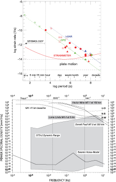
Figure 29. Sensitivity of GPS displacements compared to other geodetic methods and seismology. (Top) Strain rate comparison in the time domain. The GPS (green) is more sensitive than ultra-precise strainmeters at periods greater than a few months. The colored symbols denote different types of transients that have been measured with a GPS and InSAR including postseismic deformation (triangles), slow earthquakes (squares), long-period aseismic deformation (creep, diamonds), preseismic transients (circles), and volcanic transients (stars). High-rate GPS sensitivity extends into the seismic domain. Reproduced with permission from Nikolaidis (2002). Copyright 2002 Rosanne Nikolaidis. (Bottom) Power spectral ranges of dynamic displacement measurements for an STS-2 broadband seismometer and GPS shown with several earthquakes: 1999 Mw 7.1 Hector Mine, 2002 Mw 7.9 Denali fault, 2005 Mw 4.4 Loma Linda (below GPS sensitivity). From Genrich and Bock (2006). Copyright 2006. This material is reproduced with permission of John Wiley & Sons, Inc.
Download figure:
Standard image High-resolution image5.2.3. Seismogeodesy.
As described in the previous section, GPS displacements and seismic velocity and accelerations together provide a broad spectrum of coseismic displacements from the high frequencies to the permanent motion, although each type of data on its own has its limitations. Here we discuss the optimal combination of GPS and seismic data that minimizes their limitations and takes advantage of their complementarity, and provides a consistent set of seismogeodetic displacement and velocity waveforms. The observations, equations, and models for inverting seismogeodetic data are presented in section 2.3.
High-rate instantaneous GPS displacements can serve as long-period constraints for the deconvolution of accelerometer data, as was applied to 30 s data collected during the 1999 Mw 7.1 Hector Mine, California earthquake (Nikolaidis et al 2001), thereby increasing the temporal resolution of coseismic displacement and the observable frequency band for strong ground motions. A constrained least squares inversion technique was used to combine the GPS displacements and accelerometer data from the 2003 Mw 8.3 Tokachi-oki, Japan earthquake to estimate high-rate displacements and step function offsets in the accelerometer records, after correcting for possible spurious rotations of the accelerometers (Emore et al 2007). A multi-rate Kalman filter (Kalman 1960) used to optimally combine high-rate (1 Hz) GPS displacements and very high-rate (100–250 Hz) accelerometer observations, was applied to structural monitoring for engineering seismology (Smyth and Wu 2006). This approach was used to monitor the heavy load of the runners on the Verrazano suspension bridge at the start of the 2004 New York City marathon (Kogan et al 2008).
The multi-rate Kalman filter was first used to analyze data collected by collocated GPS and strong motion accelerometers during the 2010 Mw 7.2 El Mayor-Cucapah earthquake in northern Baja California, Mexico (Bock et al 2011). Figure 30 shows a comparison of the velocity waveform (in the vertical direction) recorded by a broadband seismometer at one collocated station and the corresponding seismogeodetic velocity waveform up to the time when the broadband seismometer clipped (Bock et al 2011). The seismogeodetic waveform provides a continuous record of the seismic motions, the dynamic component up to the Nyquist frequency of the accelerometer data collected at the station, and the progression of the static motion through to the end of the fault rupture and to its final state. Furthermore, the seismogeodetic combination is accurate enough to detect low-intensity seismic P waves and the subsequent high-intensity S waves and surface waves through to the end of the seismic shaking without interruption, a prerequisite for earthquake early warning and rapid earthquake response (discussed in the next section). GPS-only displacement waveforms are not sufficiently precise in the vertical direction, where the P wave is most pronounced; the precision of real-time GPS displacements on their own is only about 1 cm in the horizontal components and 5–10 cm in the vertical (Genrich and Bock 2006). The addition of the GPS data thus allows accurate double integration of the accelerometer data free of systematic error at the sampling rate and precision of the accelerometer measurements, dynamic displacement precision of mm or better in all three dimensions, and velocities at uncertainties of less than 0.1 mm s−1; a significant improvement on dynamic displacements from a GPS alone (previous section).
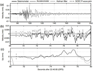
Figure 30. Seismogeodetic estimation of velocity and displacement waveforms. (a) Comparison between the vertical velocity records registered by a broadband seismometer at station WES (Southern California Integrated Seismic Network), which clipped 11 s after the onset of shaking, and the smoothed Kalman filter estimated velocities for the WES and cGPS station P494 (Plate Boundary Observatory). (b) Blowup of the same time series showing agreement between the observed velocity and the estimated Kalman velocity waveforms. The two waveforms have been offset for clarity. The Southern California Earthquake Center P wave pick denoted by vertical dashes is at 22:41:09 GPS time, or 29 s after earthquake initiation. (c) Comparison of single integration of the vertical seismometer record at WES, 100 Hz smoothed Kalman filter displacements (GPS/accelerometer), and double integration of only the accelerometer data. Note the magnitude of displacement, indicating that the broadband displacements have a precision and accuracy of about 1 mm. Reproduced with permission from Bock et al (2011). Copyright 2013 Seismological Society of America.
Download figure:
Standard image High-resolution imageThe addition of very-high-rate accelerometer mitigates the aliasing effect of lower rate GPS data (Smalley 2009). Although a GPS can be sampled at up to 50 Hz or greater, it is impractical to operate GPS receivers at this rate because of the heavy telemetry transmission load. It is sufficient to operate the GPS receivers at a rate of only 1–10 Hz, when collocated with strong-motion instruments, whose sampling rate can be comfortably recorded and transmitted at 100–250 Hz. The transition to in situ precise point positioning methods (section 2.4.2) is now becoming available, as an option with new geodetic GNSS receivers. It will allow observations at higher sampling rates, further enhancing the precision of seismogeodetic broadband displacement and velocity waveforms.
5.2.4. Earthquake early warning.
In lieu of elusive earthquake prediction (Simpson and Richards 1981), earthquake early warning (EEW) systems provide a realistic approach to partially mitigate the effects of severe shaking on people and critical infrastructure (Heaton 1985, Allen and Kanamori 2003, Gasparini et al 2007, Allen et al 2009). EEW systems have been based on traditional seismic instrumentation to provide rapid location of the earthquake source and its magnitude, and to issue a warning on the expected shaking intensity in a particular area. GPS is now being incorporated into these systems (Crowell et al 2009, Colombelli et al 2013, Grapenthin et al 2014). Here we discuss the role of seismogeodesy, particularly relevant during large earthquakes when the damage is most severe.
The simplest approach to earthquake early warning is known as frontal detection. Once strong ground shaking, starting with S wave arrival and followed by sometimes more intense surface waves, is recorded at the monitoring station closest to the earthquake source, a warning of impending strong shaking is issued ahead to those in harm's way. This is possible since the relevant information can be transmitted at the speed of light, while the travel time of destructive waves is about ~3–4 km s−1. This approach is in operation in Mexico (Espinosa-Aranda et al 1995, 2009, Espinosa-Aranda and Rodriquez 2003, Suárez et al 2009, Perez-Campos 2013), Japan (Nakamura and Saita 2007) and Taiwan (Wu and Teng 2002, Wu and Kanamori 2005, Hsiao et al 2009). The EEW system for Mexico City, for example, is based on coastal seismometers along the Guerrero seismic gap several hundred km to the southwest providing about 70 s of warning time. It, however, leaves a 'blind zone', whose radius increases by ~4 km with every second of delay in warning. A better approach with a smaller blind zone and increased warning time is to use small amplitude P waves monitored by a network of near-source seismic instruments to predict the time of arrival and the intensity of the S waves (Heaton 1985, Allen and Kanamori 2003). Depending on the distance from the source and considering that the speed of S waves is about 60% slower than P waves, the warning time may range from a few s to several min. This is the approach taken in Japan, which has the most sophisticated EEW system in the world, where the peak amplitude from the first 3 s of the P wave are used to estimate the magnitude (Hoshiba and Ozaki 2014) and then the intensity on a custom-built, 10-degree intensity scale (Hoshiba et al 2010). During the 2011 Mw 9.0 Tohoku-oki earthquake, which occurred in Sendai, Japan it took 90 s before the S waves were felt in Tokyo ~250 km from the source (Hoshiba and Ozaki 2014). Since the earthquake source region was about 100 km offshore, even someone on the coast would had a few s of warning. Strong ground shaking in the Los Angeles metropolitan area, for example, from an expected M7.9 earthquake on the southernmost point of the San Andreas fault near the Salton Sea (Fialko 2006) would be felt about 80–90 s after earthquake initiation.
There are several basic methods in use for seismic data, relying on either the time or frequency domain metrics of the recorded seismograms (Allen et al 2009). One time domain metric is the peak amplitude of the first 3 to 5 s of the P wave (Pd). Frequency domain metrics include the maximum and predominant periods of the P wave referred to as  and
and  , respectively. It is thought that these parameters scale to magnitude 7–8, and so magnitude can be rapidly estimated along with the origin time and location (Olson and Allen 2005). Using a ground motion prediction equation (GMPE), the expected intensity (strength of shaking) at a given site can be calculated and the warning time can be easily derived from a known Earth structure model for the region in question (Allen and Kanamori 2003). Since some of these metrics rely on displacement, it is necessary to singly integrate the broadband velocities or doubly integrate the accelerations. However, as the earthquake magnitude increases, integration in real time becomes more problematic introducing long period biases (described in the previous section) to the displacement waveforms (Boore and Bommer 2005, Melgar et al 2013b). Furthermore, it has been observed that the scaling relationships break down at higher magnitudes and lead to magnitude 'saturation' (Rydelek and Horiuchi 2006, Hoshiba et al 2011). This has been documented for events of M > 7. For the 1999 Mw 7.6 Chi–Chi, Taiwan and the 1999 Mw 7.1 Hector Mine, California earthquakes, and the 2003 Mw 8.3 Tokachi-oki and 2011 Mw 9.0 Tohoku-oki earthquakes in Japan, Pd is significantly lower than expected for the magnitude estimates based on empirical relationships (Wu and Kanamori 2005, Wu and Zhao 2006, Brown et al 2011). The metric
  scales better with magnitude and is less sensitive at longer distances from the source than Pd but is less precise than Pd magnitude estimates (Wu and Kanamori 2005, Brown et al 2011). Data from the 2011 Tohoku-oki earthquake indicate that the three EEW metrics have different sensitivities depending on the length of the time window over which they are estimated (Hoshiba and Iwakiri 2011). Attempts to bandpass filter acceleration waveforms, for example, at 3 − 0.075 Hz for this earthquake (Hoshiba and Iwakiri 2011) puts a limit on both the frequency-dependent and amplitude-dependent terms. Typically, systems will use multiple EEW parameters to issue an early warning in order to get a more robust warning that minimizes false alarms (Allen et al 2009).
The biggest challenge for accurate EEW during large earthquakes based on inertial instruments (seismometers and accelerometers) stems from magnitude saturation. The reason for this saturation is debated. Considering that large earthquake ruptures can last well in excess of 100 s, at issue is if measurement of the first few s of the earthquake source process contains information on whether the event will grow to a large magnitude. Thus, there is a question of whether the earthquake's final size is pre-determined once rupture starts. The argument is unsettled by either theory or observation, and studies that suggest rupture is deterministic (Olson and Allen 2005) and that it is not (Rydelek and Horiuchi 2006); each show plausible results. One of the key issues is the reliability of long-period measurements used in deriving the scaling laws of EEW; as discussed before at the longest periods, strong-motion data may have systematic errors due, for example, to spurious instrument tilts. Using the  metric for the first 3 s of seismic data for many earthquakes between M 3 and 8 indicates a magnitude scaling relationship with uncertainties of ~1 magnitude unit (Olson and Allen 2005). The number of earthquakes for which seismogeodetic displacements are available is small. However, they support the hypothesis (Olsen and Allen 2005) that P wave observations of the first few s of an earthquake can determine its final magnitude (Crowell et al 2013). Considering that there may be an earthquake nucleation phase (Ellsworth and Beroza 1995, Beroza and Ellsworth 1996), the validity of magnitude scaling has important implications for EEW systems. One possible explanation for the existence of a scaling relationship is that the probability of future rupture is proportional to the initial stress drop (i.e. large earthquakes have a larger initial energy release) (Zollo et al 2006). These results would contradict the cascade model of earthquake rupture, where slip starts on a small patch for both small and large earthquakes and then grows if local conditions on the fault are favorable. On the other hand, another study (Rydelek and Horiuchi 2006) could not arrive at a scaling relationship for earthquakes greater than magnitude 6 in Japan, so this remains a controversial issue. Since seismogeodetic Pd appears to be more robust than seismic Pd when including larger earthquakes, the issue may be clarified with a growing catalog of earthquakes recorded at collocated GPS and strong-motion sites. However, there is some evidence that due to the complex source mechanisms for great earthquakes, there exists non-linearity in scaling relationships based on observations of the 2011 Mw 9.0 Tohoku-oki (Simons et al 2011) and the 2012 Mw 8.6 Sumatra earthquakes (Meng et al 2012).
As described in the previous section, seismogeodetic waveforms estimated from a combination of GPS and strong-motion accelerometer data have an important role to play here. They are accurate enough to detect P waves for earthquakes of magnitude 4.5–5.5 or greater in the near-source region (Geng et al 2013), they do not clip in the near-source unlike broadband seismometers (figure 30), and most importantly as shown below, they are resistant to magnitude saturation. An example of a seismogeodetic-based EEW and rapid response system is shown in figure 31.
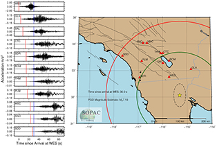
Figure 31. Example of earthquake early warning. The 100 Hz seismogeodetic displacement and velocity waveforms were analyzed retrospectively in simulated real-time mode for the 2010 Mw 7.2 El Mayor–Cucapah earthquake in northern Baja California, Mexico. On the left are shown the velocity waveforms at 12 GPS/seismic stations sorted by increasing distance from the epicenter (star with one-sigma error ellipse on the map). The continuous red vertical line denotes the current epoch. The preceding red lines indicate when the P wave was detected at each station. Once four stations have triggered, an estimate of the hypocenter can be made and the propagation of P and S waves can be determined, as shown by the partial circles, with the S wave trailing the P wave. In this scenario, it would take the S wave front about 80–90 s until it arrived in the heavily populated regions of Riverside and Los Angeles Counties. A video showing the complete sequence is given in the supplementary material (stacks.iop.org/RoPP/79/106801/mmedia). Shown here is one frame at 30 s after the earthquake origin time using peak ground displacement (PGD) magnitude scaling (109) providing an estimate of Mw 7.18,.02 magnitude units smaller than the final magnitude. Prepared by Dara Goldberg.
Download figure:
Standard image High-resolution imageThe magnitude scaling relationship using the Pd metric for seismogeodetic data can be expressed as a function of moment magnitude ( ) and epicentral distance (
 ) in the same form as seismic data (Wu and Zhao 2006)

The third term takes into account wave attenuation (through geometric spreading) and the reduction in ground shaking with distance R. By fitting the parameters A, B, and C through least-squares inversion for historical earthquakes, a scaling law was derived that can be used for future earthquakes (Crowell et al 2013). Thus, if this basic relationship holds up in practice as the database of historical earthquakes measured by seismogeodesy increases, the magnitude of an ongoing event that can be estimated within seconds of first arrivals at seismogeodetic stations. Comparing Pd magnitude scaling relationships derived from seismogeodetic and low-pass filtered accelerometer observations, the seismogeodetic is better able to distinguish between the magnitudes of large (7.2, 8.3, and 9.0) earthquakes. Another useful metric is the peak ground displacement (PGD) of the seismic waveform, which provides a revised magnitude estimate as more source information becomes available (Crowell et al 2013). This approach only requires GPS displacement measurements, but is more sensitive with seismogeodesy, and there is a growing number of earthquakes that have been thus observed (figure 32). The scaling relationship for PGD is slightly modified from the Pd relationship by adding a specific dependence on magnitude in the third term (compared to equation (108)),


Figure 32. Magnitude scaling relationship based on 3D peak ground displacements (PGD) for ten historical earthquakes. The lines are the predicted scaling values from the L1 norm regression of the PGD measurements as a function of hypocentral distance. From Melgar et al (2015a). Copyright 2015. This material is reproduced with permission of John Wiley & Sons, Inc.
Download figure:
Standard image High-resolution imageFigure 32 shows the PGD results for an expanded data set consisting of ten historical earthquakes ranging in magnitude from Mw 6.0 to Mw 9.0 (Melgar et al 2015) that better differentiates large earthquakes, but is available with additional delay, typically at about the time of S wave arrival, and is revised as the earthquake rupture proceeds. The delay in PGD compared to Pd is a function of the moment release characteristics, crustal structure, and locations of the seismogeodetic sensors.
5.3. Tsunami modeling and warning
Tsunamis are caused by earthquakes, landslides, and pyroclastic flows from a volcanic eruption (Intergovernmental Oceanographic Commission 2013). The latter two are generally of only local interest, although significant ocean-wide events have been postulated as a result of lateral landslides at submarine oceanic island arc volcanoes that may not be accompanied by seismic shaking (e.g. Ward 2001, Ward and Day 2001, Watts et al 2003, Masson et al 2006). Landsliding can be a secondary effect from tsunamigenic earthquakes, in addition to seafloor uplift (Tappin 2014).
Real-time GPS and seismogeodetic displacements are useful for tsunami modeling and tsunami prediction and mitigation systems on local to global scales. Now-time tsunami models can provide tsunami propagation and arrival times, geographical extent, inundation distance and height, and run-up (figure 33). For tsunamigenic earthquakes, the coseismic changes in elevation at coastal locations, which can reach magnitudes of several meters, should be considered; the added effect of increased sea-surface height from the tsunami and rapid coseismic subsidence can increase the hazard.
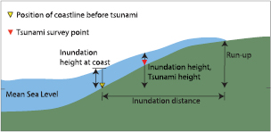
Figure 33. Tsunami wave terminology.
Download figure:
Standard image High-resolution imageCurrently, most tsunami early warning systems are focused on ocean-crossing hazards (basin-wide warning) and less so on providing accurate and robust alerts in the near-source of subduction zones, where first tsunami arrivals can occur within minutes of earthquake rupture and cause the most severe losses. For example, as described on the NOAA website, the Pacific Basin is monitored by the US National Oceanic and Atmospheric Administration (NOAA) National Weather Service's Pacific Tsunami Warning Center (PTWC) in coordination with other countries in the region as a direct response to the basin-wide destruction of the 1960 Mw 9.5 Chilean earthquake and tsunami. The West Coast and Alaska Tsunami Warning Center (WC/ATWC) was established in response to the 1964 Mw 9.2 Alaskan earthquake and tsunami. NOAA centers rely on both direct and indirect methods. The indirect method uses teleseismic waves (20 to 0.003 Hz, greater than 1000 km from the seismic instrument) recorded by global and regional networks of broadband velocity instruments, with data integrated to displacements, to produce CMT solutions that can be used by the analyst to directly issue warnings or as guidance for tsunami models. The direct method relies on NOAA's Deep-ocean Assessment and Reporting of Tsunamis (DART) buoys (González et al 2005) tethered to deep-water (4000–6000 m) ocean-bottom pressure sensors, with real-time transmission of data through satellite links (Mungov et al 2012) and deployed primarily around the Pacific Rim with GPS kinematic positioning capabilities. The pressure readings provide a proxy measurement of sea-surface disturbances, which is used to solve an inverse problem for seafloor uplift/subsidence at pre-defined locations along tectonic boundaries. The source is input to the shallow water equations with numerical dispersion to simulate physical dispersion (Titov and Gonzalez 1997) and to model tsunami propagation and generate site-specific warnings (Titov et al 2005). Direct methods are well suited to ocean-wide alerts (Tang et al 2012, Song et al 2012), but are currently of limited for local tsunamis; the alerts are not available soon enough for mitigation. DART buoys are deployed in the deep water of the abyssal plains oceanward of the subduction fronts, such that by the time a DART measurement is made the tsunami is very close, if not already at the near-source coastline.
The approach in Japan is different and is designed for the near-source region. The current tsunami early warning system is operated by the Japanese Meteorological Authority (JMA). The system was upgraded in response to the 1993 M 7.8 Hokkaido-Nansei-oki earthquake, which caused a tsunami that reached Okushiri Island in only 3 min and left 230 dead (Tatehata 1997). Tsunami propagation and inundation scenarios for different earthquake magnitudes and locations are pre-computed and stored in a database. Then, when the seismic network makes a rapid magnitude and hypocenter estimates after seismic P wave detection, the hypocentral parameters are used for a database query and the most appropriate scenario information is used to guide the warning. Later, as information from offshore GPS buoys, pressure sensors, and tide gauges becomes available, it can be utilized to update the warning (Hoshiba and Ozaki 2014). Magnitude estimates from seismic data were severely underestimated for the 2011 Mw 9.0 Tohoku-oki, Japan earthquake due to saturation (section 5.2.4) and the resulting warning significantly underestimated the tsunami heights. A similar system was designed for the Indian Ocean region, the German Indonesian Tsunami Early Warning System for the Indian Ocean, (GITEWS, Lauterjung et al 2010, Behrens et al 2010), which includes information from seismic and geodetic sensors to match pre-computed scenario information (Babeyko et al 2010).
Following the 2004 Mw 9.3 Sumatra–Andaman earthquake, several studies proposed techniques to incorporate GPS static displacements from high-rate global GPS networks into tsunami warnings, as well as for rapid estimates of earthquake magnitude (Blewitt et al 2006, Blewitt et al 2009b), while other studies used coastal (near-source) GPS observations (Song 2007, Sobolev et al 2007). One study demonstrated for the 1964 Mw 9.2 Great Alaska, the 2004 Mw 9.3 Great Sumatra–Andaman, and the 2005 Mw 8.6 Nias, Indonesia earthquakes that displacements from coastal GPS networks could be used to estimate tsunami source energy and scales due to seismically-induced seafloor uplift and coastal landsliding in real time (Song 2007), a significant improvement over traditional seismic methods. Another study (Sobolev et al 2007), proposed a similar approach of coastal GPS networks ('GPS Shields') for tsunami early warning after great subduction zone earthquakes along the Sumatra megathrust, the subduction of the Nazca plate beneath the South America plate along the Peru-Chile Trench, and the Cascadia subduction zone. Several retrospective studies have further demonstrated that with just a few GPS stations magnitude can be computed without regard for saturation from observations of peak ground displacement (Crowell et al 2013, Melgar et al 2015). Another study proposed an algorithm that produces a uniform slip model derived from replayed real-time GPS data as initial conditions for tsunami propagation (Ohta et al 2012). That study used a previously published algorithm (Tsushima et al 2009), which assumed tsunami Green's functions from unit sources of vertical seafloor displacement (Satake 1995). Further refinements to this algorithm included offshore tsunami wave measurements (Tsushima et al 2014).
Although tsunami warnings solely based on land-based GPS displacements are quite useful in now-time scenarios, the underlying tsunami models are limited due to shortcomings in rapid finite fault slip models. The resolving power of land-based data to the shallow slip responsible for large uplift and tsunamis can be quite limited (Ohta et al 2012, Melgar and Bock 2013, 2015). As is well documented by the replay of data from the 2011 Mw 9.0 Tohoku-oki earthquake, the addition of GPS kinematic displacements of near-shore buoys, near-source ocean-bottom pressure sensors (Ito et al 2011, Tsushima et al 2014), and tide gauges (Tsushima et al 2009, 2011, 2012, Maeda et al 2011) can provide improved rapid tsunami models and more detailed early warnings (Hoechner et al 2013, MacInnes et al 2013, Melgar and Bock 2013, 2015). The buoy data are transmitted through radio links and the pressure data by underwater cables. The tsunami warning system in Indonesia along the Sumatra and Java trenches for the Indian Ocean is based on real-time GPS stations on the coast and the Mentawai islands west of Sumatra, and is supplemented by near-coast GPS buoys and tide gauges (Falck et al 2010).
The methods to produce rapid tsunami models using land-based geodetic data generally involve rapid analysis of the GPS data to estimate displacements, inversion for a finite fault slip model, which is refined as wave data become available from GPS buoys and ocean-bottom pressure readings to estimate sea-floor uplift. The sea-floor uplift and topographic and bathymetric maps are used to model the tsunami propagation and then the inundation and run-up, and accordingly to issue a tsunami warning for coastal and islands adjacent to the earthquake rupture zone. Later in time, far-field seismic data can be ingested for improved emergency response. The performance of this approach for ten different source models was tested to model tsunami propagation (MacInnes et al 2013) and compared with direct deep-ocean DART buoy and coastal post-event field survey measurements (Mori et al 2012). This study found significant differences in the simulated tsunami. This is unsurprising since inversion for the earthquake source is a non-unique problem, which is dependent on the data used (seismic, geodetic, near, or far-field) and on the modeling assumptions (fault geometry and the Earth's structure). One study (Hoechner et al 2013) demonstrated rapid (within 3 min of earthquake initiation) tsunami intensity estimates in the near-source coastline from a static slip inversion using 30 s sampled GPS data, but they assumed a slab geometry and did not verify them against field measurements. Nevertheless, a rapid warning is useful even though the inundation results may not be as accurate as more physically plausible approaches using additional near-coast observations.
Tsunami waveforms from wave height from a kinematic GPS on buoys, tide gauges, and ocean-bottom pressure sensors were used to invert for the time varying finite fault slip model of the earthquake (Satake et al 2013). These data were supplemented (Romano et al 2013, Gusman et al 2012) with land-based coseismic displacements from a GPS and displacements derived from seafloor positioning (Fujita et al 2006) by five ocean-surface GPS buoys and sea-bottom acoustic transponders, fortuitously installed off the Tohoku coast between 2000 and 2004 above the 2011 hypocenter (figure 34). The seafloor displacements showed up to 24 m of horizontal motion and 3 m of vertical uplift; a land-based GPS indicated a maximum of 5 m and 2 m of subsidence, thus providing unprecedented near-source observations of a large subduction zone event (Sato et al 2011, Kido et al 2011); 31 ± 1 m of horizontal motion was recorded by an acoustic transponder within 50 m of the trench (Kido et al 2011).
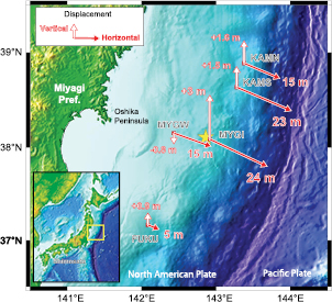
Figure 34. Horizontal and vertical coseismic displacements at four seafloor stations (red squares), associated with the 2011 Mw 9.0 Tohoku-oki earthquake. The yellow star is the epicenter. The mainland position reference is Shimosato (open triangle) shown in the insert. See also figure 13 for the velocities prior to the 2011 earthquake. Adapted from Sato et al (2011). Copyright 2011. Reproduced with permission from AAAS.
Download figure:
Standard image High-resolution imageNot all large events in a subduction zone can be assumed to happen on the megathrust, and hence it is incorrect to assume that slip is occurring on a pre-defined slab geometry. The 2012 Mw 8.6 event off Sumatra, Indonesia, was a predominantly strike-slip event that produced no significant tsunami (Satriano et al 2012). Similarly, the 2009 Mw 8.1 Samoa event was a normal faulting, outer-rise type event, which produced a sizeable tsunami with 189 fatalities (Okal et al 2010). More recently, the 2012 Mw 7.8 Haida Gwai thrust event offshore British Columbia produced a sizeable tsunami and was followed two months later by an Mw 7.5 strike-slip event on the fore-arc sliver (Lay et al 2013). It is important to characterize the style of faulting, for example by a CMT calculation (section 5.2.1) before performing the slip inversion.
We now provide an example of near-source kinematic slip inversion that tracks the time evolution of the earthquake source, and the subsequent tsunami modeling for the 2011 Mw 9.0 Tohoku-oki earthquake. The data set includes displacement and velocity waveforms from 20 land-based stations with collocated GPS and accelerometer instruments and wave gauge data from two ocean-bottom pressure sensors and six offshore GPS buoys (Melgar and Bock 2015). Utilizing tsunami wave gauge measurements for the inversion of the kinematic characteristics of the source is rather novel and assumes that tsunami propagation can be considered linear for warning purposes. This seems to be the case for the periods involved and length scales being inverted (Melgar and Bock 2015, Yue et al 2015). The first step is a line-source CMT solution (section 4.7.1) using just the land-based seismogeodetic data set to determine the type of faulting (in this case, thrust) and the geographical extent of rupture with no a priori assumptions on the fault mechanism (section 4.7.2). This is followed by two kinematic models, one using just the land-based data and the other using the complete data set (figure 35), using for each a regional 3D subduction slab model (Hayes et al 2012) discretized to sub-fault patches (Romano et al 2012). The relevant segment of the slab is chosen based on the moment release of the finite-fault (line slip) CMT solution. The tsunami Green's functions for the wave gauge data are calculated based on the seafloor deformation for 1 m of thrust and 1 m of strike-slip motion at each one of the sub-fault patches, and the tsunami waveforms are computed at the wave gauges from this unit amount of slip. The sea-surface motion time series are then taken as the tsunami Green's functions for every sub-fault and wave gauge. The respective kinematic model predicted vertical seafloor deformation then used as the initial condition for simulating tsunami propagation. If steeply sloping bathymetric features are advected large distances, they should contribute to tsunamigenesis (Tanioka and Sataka 1996, Bletery et al 2014). Therefore, the corresponding effects of seafloor horizontal motions are considered, which has a significant effect on the final model. The tsunami is propagated until 2 h after the earthquake onset time by solving the 2D non-linear shallow water equations (George and LeVeque 2006, Berger et al 2011) with the finite volume technique (LeVeque 2002). This approach provides more accurate inundation run-up heights than a static slip for this event model (figure 24), determined by comparisons with post-event land surveys (Mori et al 2012), particularly in north Sanriku, although some discrepancies between the simulated and observed run-up remain. This is a significant improvement compared to tsunami simulations from different geophysical data sets and techniques, which did not capture the large inundation levels observed along the rugged Sanriku coast between 38.4°N and 40°N (MacInnes et al 2013). It is possible that secondary sources of tsunami energy (e.g. submarine landslides, splay faults) contributed to the wave records and contaminated the models, and there is evidence that an underwater landslide could have been a significant contributor to the large inundations in north Sanriku (Tappin et al 2014). Using the full data set for the kinematic model, the peak slip is 63 m, compared to the 52 m from the land-only inversion, and the moment is 5.51 × 10²² N m (Mw 9.09) compared to 4.89 × 10²² N m (Mw 9.06). The final slip of the land-only model prefers a horizontally symmetric slip distribution about the hypocenter. For the full data set, the slip is 25 m or larger for the top 20 km of the fault restricted to the south of the hypocenter, while north of the hypocenter the large slip is confined to the shallowest 10 km. There is also noticeable shallowing of the peak slip in general with the full data set model having a larger accumulation of shallow slip.

Figure 35. Kinematic fault slip models of total slip. (a) Model from land-based seismogeodetic data; (b) model from seismogeodetic and wave gauge data. The dashed lines are depth contours of the subducting slab in km. A video showing the complete sequence is given in the supplementary material (stacks.iop.org/RoPP/79/106801/mmedia). From Melgar and Bock (2015). Copyright 2015. This material is reproduced with permission of John Wiley & Sons, Inc.
Download figure:
Standard image High-resolution imageUsing the full data set, figure 36 shows four samples from an animation depicting the inundation model in Sendai Bay, where the inundation distances were quite large (the animation is found in the supplementary material) (stacks.iop.org/RoPP/79/106801/mmedia). It shows the predicted tsunami amplitudes over the affected region at different intervals after the earthquake origin time. With increased fault model complexity and heterogeneity of the input data set, the predicted inundation and run-up compared to the survey point mean sea level elevations (Mori et al 2012) is significantly improved (Melgar and Bock 2015). The reason why a composite model of on-land and off-shore data produces better run-up models can be better understood by considering the resolution of each data set. Each data type, seismogeodetic displacement, velocity, and tsunami wave data have a different resolving power for the distribution of fault slip. This heterogeneous sensitivity can be seen in figure 37. Shown are the diagonal values of the resolution matrix (the generalized inverse of the Green's function matrix). If all the model parameters are perfectly resolved and can be independently determined, then the resolution matrix will be the identity matrix (Aster et al 2013). If the diagonal values are less than one, then the value of a particular model parameter can be affected by (and is not independent of) the neighboring model parameters. If the resolution for a particular model parameter is relatively high, then that slip value can be considered reliable. A low resolution, on the other hand, indicates that the value of the slip is likely the average slip of several neighboring sub-faults. Thus, low resolution is indicative of a smeared out model that cannot resolve sharp features. The resolution matrix for this earthquake indicates that the displacement time series are most sensitive to the slip closest to the coast and almost completely insensitive to a slip close to the trench; any trench-proximal slip on displacement-only models is likely the result of averaging on deeper faults as well. On the other hand, the velocity time series show no along-dip bias. The value of the resolution matrix is similar throughout. That is, velocity data are equally sensitive to slip anywhere on the fault. In turn, the tsunami wave observations are most sensitive to slip by the trench and, in this case, due to the station distribution, to the northern half of the fault model. Each data set used independently provides limited resolving power, while the combination affords a substantial improvement.

Figure 36. Four snapshots in time of tsunami run-up modeling of the coast surrounding an area of Sendai Bay after the 2011 Mw 9.0 Tohoku-oki, Japan earthquake. The blue dots are the locations of the survey measurements from Mori et al (2011). The model inundates 891 out of 1023 points in this region. A video showing the complete sequence is given in the supplementary material (stacks.iop.org/RoPP/79/106801/mmedia). From Melgar and Bock (2015). Copyright 2015. This material is reproduced with permission of John Wiley & Sons, Inc.
Download figure:
Standard image High-resolution image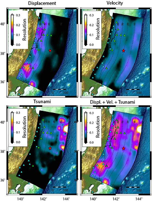
Figure 37. Resolution for a series of kinematic fault slip inversions using different input data sets. Larger values denote more sensitivity, highlighting their contributions to different portions of the subduction geometry. From Melgar and Bock (2015). Copyright 2015. This material is reproduced with permission of John Wiley & Sons, Inc.
Download figure:
Standard image High-resolution imageTo put this into perspective, the Japanese EEW response to the 2011 Mw 9.0 Tohoku-oki earthquake provided significant lessons for hazard mitigation systems and future disasters. In hindsight, reliance strictly on a single data set, in this case seismic instruments on the Japanese mainland, resulted in a severe underestimate of the actual first magnitude, Mw 7.9 (Ozaki et al 2011), on which the tsunami prediction depended. As described in this section, using just the displacement data from the existing high-rate real-time GPS network in Japan (GEONET, Sagiya et al 2000) would have resulted in an accurate magnitude estimate and a reasonable static slip model within 3–4 min of earthquake initiation; the subsequent tsunami prediction would have been much improved. The reaction time is critical since tsunami waves began to arrive in Sendai ~30 min after the earthquake initiation. Lessons learned from this tragic event have spurred increased usage of real-time geodetic and seismogeodetic monitoring in designing early warning systems.
5.4. Volcano monitoring
The GPS and other geodetic systems, in particular interferometric satellite radar interferometry (InSAR), are important in volcanology. Modeling the magmatic chambers and volcano fissures at depth from surface displacements to understand the underlying physical processes of magmatism is analogous to the modeling of crustal deformation at the larger scale of geologic faults. Unlike earthquakes, however, volcanic eruptions are often preceded by detectable precursory motion, from periods of minutes to months, which can be used to assess risk and issue warnings to those in harm's way. Furthermore, it is important to relate localized volcanic deformation to regional tectonic motion, as volcanic arcs are commonplace in subduction zones (Stern 2002) and are generally a consequence of partial melting of the mantle induced by downgoing slabs. For example, the Cascadia subduction zone, which includes a volcanic arc of ten volcanoes along the Cascade ranges in the western US, is a complicated tectonic and volcanic region with newly discovered transient deformation at local and regional scales. To put the volcanic risk in this region into perspective, the Mount St. Helens stratovolcano suffered a major explosive eruption in 1980 with accompanying loss of life and property, continuing activity during 1981–6 producing a new lava dome, and eruptions in 2004–8 with a cumulative volume of lava of nearly 100 million cubic meters (Iverson et al 2006).
Geodetic observations of a volcano's crater rim and flanks complement seismic observations (Chouet 2003), magmatic gas emission rates, and well water changes, by measuring the spatial and temporal patterns of deformation (uplift and horizontal motion) of the volcano edifice due to magmatic intrusion that may or not be accompanied by seismicity (Dzurisin 2003, 2006). Early geodetic observations used electronic distance measurements (EDMs) for this purpose (Langbein 2003); these were supplemented and later supplanted by in situ sGPS and/or cGPS and satellite interferometry, including the InSAR and persistent scatterer methods (Amelung et al 2000, Ferretti et al 2001, Hooper et al 2004). As with tectonic deformation, cGPS observations provide detailed temporal resolution of surface motion, while InSAR provides detailed spatial resolution. Additional geodetic measurements on volcanoes may include tiltmeters, borehole strainmeters, and gravimeters (Dzurisin 2006). Technological improvements in geodetic technology have also increased the timeliness of observations of surface deformation. Together, finer resolution on both spatial and temporal scales and real-time access to data improve hazard mitigation efforts through precursory and more rapid modeling of the underlying physical processes of the volcanic source. Furthermore, finer resolution requires increasingly sophisticated inverse models in order to fit the observations of geodetic and other data. The simplest models of volcano deformation include point/spherical ('Mogi') sources and closed pipes (figure 38), ellipsoidal chambers, and fault dislocations within homogeneous and elastic media. The inversion of geodetic and other data may require more complex models with viscoelastic rheology and inhomogeneous materials. One study modeled sill-like magma intrusions by a horizontal circular crack in a semi-infinite elastic solid for magmatic processes of calderas in Socorro, New Mexico, and Long Valley, California (Fialko et al 2001a, 2001b). Another study modeled several months of continuous data leading up to the 2008 eruption of the Okmok volcano in the Aleutian island chain (Freymueller and Kaufman 2010). They observed 6–7 months of precursory inflation leading up to the main eruptive event, which then resulted in deflation of the volcanic edifice. Their Mogi source model showed that post-eruptive deflation was due to a source about 2.1 km below sea level. Reinflation was observed as quickly as three weeks after the main eruption and suggested that there was a transfer of magma from a deeper to a shallower body at mid crustal depths once the eruption was complete. Though they were limited by the number of available far-field stations, they hypothesized that what they observed was the concurrent behavior of two sources, one producing deep deflation and another shallow inflation.

Figure 38. Volcano monitoring. (Left) Example of two volcano deformation sources used to model surface deformation: A Mogi source at 9 km, and a closed pipe extending from 6.5 to 11 km depth. The initial volume of both sources is chosen to be 0.88 km3 and both volumes are assumed to increase by 0.018 km3. Note that the inversion model parameters were chosen to approximate those inferred for the magma body that fed the 18 May 1980 eruption of Mount St. Helens (Scandone and Malone 1985), and that eruptions with this increase in volume are quite common. (Right) Calculated surface displacements and strains caused by a volume change of 0.018 km3 in each source. The uplift patterns produced by an inflating Mogi source and a closed pipe are very different in proximal areas (here within ~1/2 source depth) but not in distal areas. Thus, to distinguish between these two models requires a distribution of cGPS stations in the proximal areas, as well as the distal areas. Adapted from Dzurisin (2003). Copyright 2003. This material is reproduced with permission of John Wiley & Sons, Inc.
Download figure:
Standard image High-resolution imageGPS observations are being conducted on a growing number and type of volcanoes worldwide, in particular in the Pacific Rim, or 'Ring of Fire', which contains the world's major subduction zones—the area has produced nine of the largest ten earthquakes in recorded history (when including the subduction zones of Indonesia), as well as in the Mediterranean (in particular, southern Italy and Greece), Japan, Iceland, and the Caribbean. For example, geodetic observations (EDM, GPS, tilt and radar interferometry), along with seismicity, and gas emissions of the Merapi stratovolcano in central Java, Indonesia provided precursory signals for eruptions in late 2010 that were proportional to the size and intensity of the eruption (Jousset et al 2012). Although almost 400 deaths were reported, the timely forecasts of the magnitude of the eruption phases by the Indonesian Center of Volcanology and Geological Hazard were estimated to have saved 10 000–20 000 lives, with the displacement of more than a third of a million people. The explosive eruptions in April 2010 of the Eyjafjallajökull stratovolcano, Iceland, spewed volcanic ash to heights of several km, requiring hundreds of people to be evacuated and disrupting air travel in Europe for several weeks. Precursory GPS and InSAR observations recorded a 0.05 km3 magmatic intrusion, growing over a period of three months in a temporally and spatially complex manner and rapid deformation of >5 mm d−1 in the month prior to the first eruption (Sigmundsson et al 2010).
There are a growing number of volcanoes being monitored by modern geodetic methods. A partial list includes Hawaiian-type volcanoes in Kilauea, Hawaii (see the discussion and references below), composite stratovolcano Mount Etna, Italy (Palano et al 2008, Bonforte et al 2008, Aloisi et al 2011, Bruno et al 2012), Strombolian-type volcanoes in Stromboli, Italy (see the discussion and references below), stratovolcano Mount Erebus, Antarctica (Aster et al 2004, Willis 2008), central dome cluster volcano Augustine, Aleutian Arc, Alaska volcano (Cervelli et al 2006, Mattia et al 2008), the complex Three Sisters volcano, Cascadia Range, US (Dzurisin et al 2006, 2009), the Soufrière Hills stratovolcano, Montserrat (Mattioli et al 2010), and the Okmok caldera in the Aleutian island chain (Freymueller and Kaufman 2010). The most intensive geodetic (and other geophysical) monitoring occurs in Japan; e.g. the 1990–5 eruption of the Unzen complex stratovolcano (Nishi et al 1999, Nakada et al 1999) in the Izu peninsula, where magmatic-tectonic activity in the late 20th century encompasses more than a dozen earthquake swarms associated with magmatic intrusions, broad uplift, and several offshore eruptions (e.g. Cervelli et al 2001), and the complex Mt. Asama volcano (Takeo et al 2006).
Annual sGPS surveys were first applied to monitoring the resurgent dome at Long Valley caldera, California (Dixon et al 1993, Marshall et al 1997) and later by cGPS monitoring (Dixon et al 1997). The first three years of observations collected at two stations on the resurgent dome showed a major inflation atop a magma chamber on the west side of the dome at a depth of 4–7 km, assuming a simple point source model. Applying more complex models of the underlying physical volcanic processes was limited by inadequate spatial coverage, a situation that is remedied by the addition of InSAR observations (e.g. Lundgren et al 2013). InSAR is limited temporally and access to data is more restricted, thus it is less useful for short-term prediction since the repeat times for a satellite to image a given point again can be as long as a month. However, vertical signals from GPS can be obscured by non-volcanic effects such as seasonal snow cover and changes in groundwater due, for example, to nearby geothermal power plants (Dixon et al 1997). A more recent study with a richer data set (Liu et al 2011a) inverted a combination of InSAR and continuous GPS observations from 1996 to 2009 at the Long Valley Caldera using a spherical source and dipping prolate spheroid model (Fialko et al 2001a) for volcanic source geometry and magmatic volume change for four distinct deformation episodes of uplift and subsidence over that time interval. The post-2000 events of uplift and subsidence appear to result from the same prolate spheroid source at a depth of 6–8 km with a low total volume change, compared to an earlier 1997–8 uplift (inflationary) episode with a steeper source geometry and significantly greater volume change rate (Fialko et al 2001a, Langbein 2003). Along with decreased seismicity during the post-2000 events, the surface deformation patterns imply that the probability of eruption is low (Liu et al 2011a).
Volcano monitoring by the US Geological Survey and others has a long history within the Hawaiian archipelago, including the active Kilauea shield and hotspot volcano, Mauna Kea, the Hualalai volcanoes on the island of Hawaii, and the Haleakala (East Maui) volcano on the island of Maui. The south flank of the sub-areal Kilauea volcano has generated frequent large earthquakes, which motivated annual GPS surveys starting in 1990, eventually growing into a network of more than 60 monuments, including cGPS observations (Owen et al 1995, 2000a). Data collected in the period 1990–1996 showed motions up to 80 mm yr−1 to the south–southeast, a few kilometers south of the summit caldera, which was modeled by a homogeneous elastic half-space model (section 4.5.3) to reveal a deep rift opening along the upper east rift zone, a fault slip along a subhorizontal fault near the base of the volcano at rates of 230–280 mm yr−1, and deflation near the summit caldera (Owen et al 2000b). Observations taken during the 1997 eruptive event indicated a precursory signal starting 8 h before the eruption, indicating rift intrusion extending to a fairly shallow depth (2.4 km) due to deep rift dilation and slip on the south flank of the underlying fault, but there was no precursory inflation signal of the summit, ruling out magma storage overpressurization (Owen et al 2000b). Transient displacements of as much as 15 mm were recorded in November 2000 over a period of 36 h with an equivalent moment magnitude of 5.7 and interpreted as an aseismic fault slip on a shallow-dipping thrust fault at a depth of 4–5 km beneath its south flank with a maximum slip velocity of about 60 mm d−1 (Cervelli et al 2002). Similar ~2 d events were recorded in September 1998, July 2003, and January 2005, all accompanied by an increased level of microseismicity, whose cumulative moment for each episode could not accommodate the surface displacements; hence, evidence of a 'silent earthquake' or 'slow slip' (Segall et al 2006), a phenomenon first observed in subduction zones in Japan, Mexico, and Cascadia (section 4.8.3). The last event, and the most energetic, preceded the earthquake swarm, implying that the earthquakes were triggered by increased stressing caused by the slow slip. Coulomb stress considerations (section 4.6) that constrained the slow slip event to the same depths (~7 km) were determined through dislocation modeling of the microseismicity and were consistent with the surface GPS displacements. Considering that triggered small earthquakes may lead to large destructive earthquakes, observations of slow slip through analysis of surface GPS displacements can reveal otherwise difficult to detect triggered microseismicity, and may therefore serve as a useful and complementary metric for assessing increased hazards at subduction zones (Segall et al 2006). Most recently, significant inflation of the summit of Kilauea preceded the 5–9 March 2011 Kamoamoa fissure eruption along the east rift zone observed by GPS and InSAR over a several months period prior to the event (Lundgren et al 2013).
It has been argued that the continuous GPS deployment on Kilauea can observe possible aseismic catastrophic flank failures as precursory signals to destructive Pacific Basin-wide tsunamis (Ward 2001). At another location, a real-time GPS network was installed on the edifice of the Stromboli volcano in the Aeolian Islands, Italy to monitor tsunamigenic landslides and the collapse of the volcano's northwest flank, documented in the historical record (Mattia et al 2004). Observations were initiated several days after it erupted on 28 December 2002 (Bonaccorso et al 2003); the eruption caused a tsunamigenic landslide on its northwest flank two days later and its effects were felt in the coastal areas of southern Italy. The Stromboli volcano is characterized by persistent but moderate ('Strombolian') explosive activity within its shallow magma chambers, making the installation of sensors hazardous. The GPS data and seismicity were used to rule out a tsunami warning after capturing a vent migration episode over a 2 d period in February 2013. In April 2003, data were collected during a paroxystic explosion episode that ejected basaltic rocks, destroying houses and walls on the island and causing significant damage to the island's monitoring networks. The dangers of deployment on volcanoes was further highlighted when one of the GPS stations was destroyed by lava several days after installation, but it succeeded in transmitting 1 Hz data up to its demise, capturing 90 s of explosive activity. The GPS displacement data were inverted to identify three phases of the eruption that were modeled by assuming a homogeneous, isotropic, and elastic half-space (section 4.5.3) (Okada 1985).
As a final example of volcano monitoring, the active Santorini Caldera, a volcanic complex in the southern Aegean related to subduction along the Hellenic arc, was the location of a massive eruption and ensuing tsunami in about 1650 BCE, which devastated the Minoan civilization and created the mostly submerged current edifice. In early 2011, after a 50 year period of quiescence, possible precursory signals were detected from increased microseismicity and anomalous displacements, recorded by a dense network of 19 sGPS and five cGPS stations (figure 39) established beginning in 2006 (Newman et al 2012). The most recent significant eruptions on Santorini took place in 1939–1941 and 1950. The last year of GPS displacements showed that the caldera edifice had extended laterally from a point inside its northern segment by about 140 mm and was expanding at a rate of 180 mm yr−1 (figure 40). Spherical source models showed that the source at about 4 km depth has no significant source migration, but has expanded by 14 million m, with a possible N-S elongation of the volumetric source. To better image the source, the GPS data were supplemented by InSAR satellite line-of-sight surface displacements over the same period, and also by triangulation data taken in 1955, which indicated that the only significant deformation began in the 2011 inflation episode, and suggested that the dynamics of the deep reservoirs may play a greater role than expected by delivering magmatic pulses to the shallow chambers, which can last on the order of a century (Parks et al 2012). Combining the GPS data and additional InSAR line-of-site displacements using the method of persistent scatters (Ferretti et al 2001) indicated a large inflation signal, up to 150 mm yr−1, which was modeled as a Mogi source (figure 38) at a depth between 3.3 km and 6.3 km, and with a volume change rate in the range of 12–24 million m3 yr−1. This later study suggests that the intense geophysical activity that started in the 2011 episode has begun to diminish since the end of February 2012 (Papoutsis et al 2013). Indeed, at the present time (circa August 2015) the caldera has not experienced an eruption.

Figure 39. Map view of the (a) horizontal and (b) vertical displacement fields on Santorini caldera with scaled seismicity (M ⩽ 3.2; blue) in 2011. 19 sGPS and 5 cGPS (magenta diamonds) show near radial displacements between their last observations in 2010 and late August 2011. (c) The temporal evolution of seismicity (M ⩾ 1.0) and GPS as represented by the eastward component of station NOMI are also shown. Note that the cumulative number of earthquakes mimics the inflation shown. See also figure 40. From Newman et al (2012). Copyright 2012. This material is reproduced with permission of John Wiley & Sons, Inc.
Download figure:
Standard image High-resolution image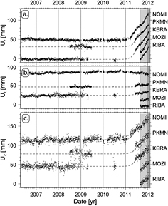
Figure 40. Time series of five cGPS stations on the Santorini caldera (figure 39) from 2006 showing the relative motion in the (a) radial (Ur), (b) transverse (Ut), and (c) vertical (Uz) directions. Stations RIBA and MOZI were installed in late August 2011 and are denoted by the vertical gray bar. Reproduced from Newman et al (2012). Copyright 2012. This material is reproduced with permission of John Wiley & Sons, Inc.
Download figure:
Standard image High-resolution image6. Atmospheric monitoring
6.1. Troposphere
6.1.1. Motivation.
The GPS signal is significantly delayed by the neutral (non-dispersive) atmosphere, encompassing the troposphere and stratosphere up to a height of about 50 km, and is modeled by the troposphere delay in the zenith direction at station i,  (9). Since the neutral index of refraction in the atmosphere is a function of atmospheric water vapor, pressure, and temperature,
  can be mined for short-term weather forecasting and long-term climate studies. Estimating water vapor in the troposphere above a ground-based network of GPS stations is referred to as GPS meteorology; about 95% of water vapor is below 5 km. Each GPS receiver records data down to an elevation angle of about 7° within an inverted cone centered on the receiving antenna; observations are not used below this elevation angle since the line-of-sight mapping function from station i to satellite j (
 (9) is inaccurate this low above the horizon (Fang et al 1998). Furthermore, the high spatial variability of water vapor is especially pronounced in the planetary boundary layer (~2 km), which is preferentially sampled at elevation angles below 5–7 degrees. Typically, a troposphere delay parameter is estimated in the zenith direction at intervals of 5–30 min. As discussed in the next section, ZTD is a sum of a hydrostatic component (zenith hydrostatic delay—ZHD) and a wet component (zenith wet delay—ZWD). The ZHD is on the order of 2.3 m and increases by about a factor of 4 near to the horizon. It can be modeled very precisely by surface pressure measurements at the GPS station with a precision of at least 0.3 hPa corresponding to a precision of about 1 mm in delay (note that 1 mb = 1 hPa). The ZWD is directly related to the amount of atmospheric water vapor above the GPS station and typically ranges from ~10–150 mm, but can vary from a few mm in cold dry conditions to more than 450 mm in very humid conditions. However, it cannot be accurately modeled. Therefore, after correcting for the ZHD, the estimated parameter ZTD in the inversion (15) is effectively the ZWD. The ZWD is linearly related to precipitable water (PW) defined as the height of an equivalent column of liquid water if all the water vapor contained in a vertical column were completely condensed. The PW can be extracted from ZWD using in situ surface pressure and temperature measurements. This is the basis of GPS meteorology, as discussed in section 6.1.3. The use of long time series of ZTD and PW for climate change research is discussed in section 7.5.
6.1.2. Troposphere parameter estimation.
The change in path distance of the GPS signal is given by Bevis et al (1992)

where S denotes the actual curved distance of the refracted ray path, r is the straight-line geometric distance from the satellite to the GPS antenna that the wave would travel if in vacuum, and  is the index of refraction. The integration is formally from the location of the GPS antenna on the Earth's surface to the height of the satellite, but effectively to the top of the atmosphere. The first term on the right is due to the slowing of the signal, while the second term is due to the much smaller bending of the signal (~1 cm at 15° elevation) and is usually ignored so that

In space-based GPS meteorology (radio-occultation or limb sounding, section 7.5.2), bending of the signal at low elevation angles is much more significant, and is fundamental to the retrieval method for refractivity. However, for ground-based GPS meteorology, it is sufficient to integrate over r such that (Saastamoinen 1973)
where  is the varying angle between the zenith and the tangent to S with value
  = 0 at the surface. Second order geometrical deviations can be accounted for in an elevation angle dependent mapping function. Since the deviation from unity is very small at radio wavelengths, the index of refraction is replaced by

where  is called the refractivity. Making a simplifying assumption about the dependence of N on height

where R is the ideal gas constant for dry air,  is the index of refraction for pressure
  and absolute temperature
  at the GPS ground antenna, and g is the value of gravity at the centroid of the atmospheric column above the GPS station (Saastamoinen 1973). Since on average the atmosphere is in hydrostatic equilibrium, any pressure (including
  ) measured within the vertical column of unit cross section is equal to the total weight of the air in the column. The total signal delay can be approximated by
where  is the zenith angle at the surface, and
  is the partial pressure of the water vapor in hPa, with
  in hPa and
  in K.
in K.
For GPS analysis, the total troposphere delay is expressed as a function of its hydrostatic and wet components through an expression for the refractivity of moist air (Thayer 1974)
where  is the partial pressure due to water vapor,
  is the partial pressure of dry air,
  and
and  are the compressibilities of dry air and water vapor (deviations from ideal gas behavior), respectively, and
  are constants, which have been determined experimentally (Smith and Weintraub 1953, Thayer 1974, Davis et al 1985, Bevis et al 1992, Rüeger 2002, Aparicio and Laroche 2011, Healy 2011), where
  = (77.604 ± 0.014) K hPa−1,
  = (64.79 ± 0.08) K hPa−1,
  = (3.776 ± 0.004) × 105 K2 hPa−1. The first term of (116) reflects the partial pressure of the dry air (mainly N2 and O2) and the second term the nondipole component of the water vapor refractivity. The second term is due to the induced dipole moment of water vapor. The third term is related to the permanent dipole moment of a water molecule. The three terms can be rearranged (Davis et al 1985; equation (A7)) so that the new first term (
 ) is dependent on the total mass density of the atmosphere
  and not on the wet/dry mixing ratio (
 is the specific gas constant for the hydrostatic component); the second term has a new constant
  (17 ± 10) K hPa−1, and the third term is unchanged. Integration over height yields the zenith hydrostatic delay

The hydrostatic term depends on surface pressure, which has a much larger spatial scale of variation in the atmosphere than water vapor, so the wet term tends to vary much more rapidly than the hydrostatic term. The zenith hydrostatic delay is inversely proportional to a function of  and
and  , which is approximately equal to gravity
  at the center of mass of the vertical column above the station at geodetic latitude
  and geoidal height H (figure 44). Assuming typical atmospheric conditions and uncertainties, one arrives at (Saastamoinen 1973)
This expression (first developed for very long baseline interferometry, where large radio telescopes receive signals from quasars and other extragalactic radio sources) is the one recommended for GPS analysis by the International Earth Rotation and Reference Systems Service (IERS; Petit and Luzum 2010).
As seen in (115), the total delay varies approximately as the secant of the zenith angle and so becomes quite large near the horizon. In forming the computed observables for inverting the GPS observation equations (9) and to achieve geodetic accuracy, it is necessary to compute the atmospheric delay along the line of sight to each satellite as part of the linearization of the GPS observables (6), because there are significant correlations between the station position and troposphere delay parameters as well as with site multipath effects (Bock et al 2000). Calculating the atmospheric delay along the line of sight requires specification of a zenith delay mapping function to account for the bending of the ray path, which was only approximated in equations (112)–(114). The mapping function is split into a hydrostatic component  and wet component
  to account for different scale heights in the atmosphere, and expressed in terms of elevation angle, el

where ZHD is given by (118) and ZWD is estimated through the GPS inversion (9). Since the advent of radio observations of celestial objects for geodetic applications, several empirical mapping functions have been developed under a variety of assumptions (Davis 1986, Lanyi 1994, Niell 1996). A convenient way to express the mapping function is through a 3-parameter (a, b, c) continued fraction (Marini 1972, Davis et al 1985) of the form
Among mapping functions that use external numerical weather models, the Vienna Mapping Function 1 (VMF1) (Boehm et al 2006a) is recommended for GPS analysis by the IERS Service (Petit and Luzum 2010). It is based on ray traces through the refractivity profiles of the 2001 European Centre for Medium-Range Weather Forecasts (ECMWF) prediction model at 3° elevation and empirical equations for the b and c coefficients (120), and is available within 6 h of real time on a global 2.5° × 2.0° degree grid, as well as for a list of global stations of the IGS. For real-time applications it is preferable to use a mapping function that only requires the geographic location of the station and the date of the observations. This is available through physically realistic empirical global mapping functions (Niell 1996); the Global Mapping Function (GMF, Boehm et al 2006b) is based on the climatological average of the ECMWF re-analyses, so in methodology it is consistent with VMF1. The most recent slant delay models (Lagler et al 2013, Boehm et al 2015) have improved spatial and temporal variability compared to earlier models. They provide pressure, temperature, lapse rate, water vapor pressure, and mapping function coefficients at any station for use as a priori values, resting upon a global 5° grid of mean values, and annual and semi-annual variations in all parameters. Comparisons of the model (Lagler et al 2013) with in situ measurements of pressure at about 350 well-distributed global stations yields a median of individual station root mean square (RMS) differences of 1.0 hPa. The model provides RMS values below 5 hPa (equivalent to 1.3 mm station height error) for 95% of all stations. The newest model (Boehm et al 2015) has an improved capability to determine zenith wet delays. In terms of zenith total delays, the globally averaged bias is below 1 mm and the RMS difference is about 3.6 cm. Both empirical models only require the day of the year and approximate station coordinates to estimate slant delay.
It should be noted that tropospheric delay estimation may also include the estimation of horizontal gradient parameters to model azimuthal asymmetries in the atmospheric refractive index due to atmospheric conditions, which can be as large as 50 mm of delay at a 7° elevation (Macmillan 1995). This adds a third term to (119); see also (9), ![$m{{f}_{g}}(e)\left[{{G}_{N}}\cos \alpha +{{G}_{E}}\sin \alpha \right]$](https://content.cld.iop.org/journals/0034-4885/79/10/106801/revision1/ropaa04ddieqn396.gif) , with gradient mapping function
, with gradient mapping function  , gradient parameters G in the north and east components, and azimuth
  (Chen and Herring 1997). The gradient parameters may be estimated from once every few minutes to once every few hours. For completeness, it should also be noted that a stochastic constraint may be applied to consecutive troposphere delay parameters in the GPS parameter inversion (9), which can be accomplished through weighted least squares or a simple Kalman filter formulation (Bar-Sever et al 1997). The choice of stochastic process is subjective; it should not over-constrain the estimated parameters during periods of high (~5 mm h−1) PW changes.
6.1.3. GPS meteorology.
In the previous section, we treated the troposphere delay as a 'nuisance' parameter, which needs to be accounted for in precise GPS positioning. Here we describe the physics of GPS meteorology from a network of ground-based GPS stations and give an example of its use in forecasting extreme weather. In GPS meteorology, it is typical (Gutman et al 2004) to tightly constrain the station positions at their true-of-date (ITRF) coordinates and to take as fixed the satellite orbital elements at the epoch of observation estimated in a separate process or obtained from a provider such as the IGS (section 2.1). Once the modeled ZHD has been differenced from ZTD (i.e. ZWD = ZTD-ZHD), one can then relate PW to the ZWD by (Bevis et al 1994)
where  is the density of liquid water,
  is the specific gas constant of water vapor, and
  and
and  are the ratio of the molar masses of water vapor and dry air, respectively. The coefficients
  are from (116).
  is the weighted mean atmospheric temperature (Davis et al 1985)
Assuming an empirical linear relation between the surface temperature and mean temperature of the atmosphere,  can be approximated from surface temperature measurements at the GPS station and synoptic surface temperatures from nearby stations or numerical weather models (Bevis et al 1994). The accuracy of the GPS-derived PW is approximately proportional to the accuracy of
  (Wang et al 2005). The relative error of PW due to errors in
  is given by

since  is about 60 micro K−1, indicating that on average from 240 K to 300 K the 1% accuracy in PW require errors in
  less than 2.74 K (Wang et al 2005). Nevertheless, in practice errors due to
  the values are almost always smaller than the uncertainties in the ZTD estimate. For now-time GPS meteorology applications, it is preferable to rely on the strong relationship between
  and surface temperature readings, by approximating it from collocated temperature sensors or nearby (~several km) weather stations recordings. The RMS error of
  ranges from ~2–5 K, corresponding to an uncertainty 0.7–1.83% in
  (Wang et al 2005), and has a bias at night. For the post-processing of GPS data for climate studies (section 7.5), global temperature and humidity profiles from re-analyzed numerical weather models such as ECMWF are preferred, and are used for GPS stations that do not have in situ or nearby synoptic readings, or as an external check, since the accuracy of the relationship between surface temperature and
  can vary both temporally and spatially and with extreme weather.
Based on 2 hourly PW estimates over a period of 7 years from over 250 globally-distributed GPS stations, the total PW error was found to be less than 1.5 mm including errors in ZTD of 4 mm, 1.3 K in TM, and 1.65 hPa in surface pressure (Wang et al 2007). This result was reinforced by GPS-derived PW observations across Europe (Emardson and Derks 2000) and other more focused studies (Haase et al 2003). Comparisons of the GPS-derived PW with collocated radiosonde and microwave water radiometer estimates show a mean difference of about 1 mm (Wang et al 2007). The accuracy of GPS PW estimates, then, are on the order of 1–2 mm (as a rule of thumb, 1 mm in PW is equivalent to about 6.4 mm in ZWD and can vary by ~20%) (Bevis et al 1994).
To illustrate the application of GPS meteorology to the short-term forecasting of extreme weather, we present an example of a regional GPS network in southern California with a typical station spacing of 30 km supplemented with surface meteorological pressure and temperature sensors. The network was used by a NOAA's Weather Forecasting Office to issue a flash flood warning during the North American Monsoon in the summer of 2013 (Moore et al 2015). The summer monsoon season in southern California and the southwestern US is due to the rapid evolution of surges of low-to-mid level moisture from the Gulf of California and the Gulf of Mexico. Increasing levels of PW interact with the mountainous terrain and can cause severe thunderstorms followed by dangerous flash floods. These rapidly evolving low-to-mid level regional moisture surges can be particularly difficult to detect using satellite, radar, and surface dewpoint observations. Available to the forecasters for this region, once every 12 h, are radiosonde measurements of water vapor, numerical weather models that are limited in predictive ability during these rapidly-varying weather conditions, and the described ground-based GPS measurements of PW. The monsoon conditions for an event in 2013 produced heavy rainfall, flash flooding, and debris flows in Riverside and San Diego counties. Precipitation totals over 1 h exceeded the 1000 year recurrence levels on 22 July at Llano, California in the Antelope Valley, where vehicles became stuck due to flash flooding. Other local storm reports indicated debris flows exacerbated by recent wildfire activity, vehicles trapped on a roadway between two flooded locations, and bowling ball-sized rocks and 1 m deep flood deposits covering about 24 m of a road. Animations of the GPS PW during the monsoon event, alongside weather model-derived PW, radar reflectivity, and rainfall data are available in the supplementary material (stacks.iop.org/RoPP/79/106801/mmedia).
6.2. Ionosphere: earthquake and tsunami observations
6.2.1. Motivation.
The effect of the ionosphere on the propagation of radio waves is dispersive and inversely proportional to frequency. Hence, the GPS constellation transmits data on two frequencies (L1 and L2, section 2.1) so that, at least to the first order, the effect of ionospheric refraction on positioning is eliminated by a particular combination of dual-frequency phase or pseudorange observations (10). The differential delay is proportional to the path integral of the electron density  along the raypath s between the antenna phase center and the satellite (the ionosphere is at an altitude of about 50 km to 1000 km). This cumulative quantity known as total electron content (TEC) is derived as:

and is expressed in TEC units (TECU), where 1 TECU = 1016 electrons m−2 (Langley 1996). TEC can be estimated from the GPS observables (section 2.3) as
where A = 40.28 m3 s−2, N is the integer-cycle phase ambiguity,  is the satellite phase bias,
  is the station phase bias, and c is the speed of light. This relationship can then be used to obtain the ionospheric range correction for either frequency
However, TEC variations in GPS signals can be exploited to detect perturbations in the ionosphere caused by a wide variety of sources. Internal sources include atmospheric perturbations from earthquakes, tsunamis, volcanic eruptions, or deep convective events (large hurricanes or tornadoes). External sources as such geomagnetic storms, aurora, and plasma instabilities, and man-made sources such as explosions and rocket ascents are also observable. This analysis can be performed at ground-based GPS receivers by estimating the relative change of the ionospheric TEC over time directly from the GPS phase observations. The GPS approach was first used to detect small electron density and TEC variations generated by surface displacements resulting from the 1994 M6.7 Northridge, California earthquake (Calais and Minster 1995, 1998).
The ionosphere is a layer of free electrons that exists from about 50 km to 1000 km in the atmosphere. Short wavelength radiation from the sun (x-rays, ultraviolet, etc) is energetic enough to dislodge electrons from neutral gas atoms and molecules. At these altitudes, the atmosphere is sufficiently thin that there are not enough positive ions to re-capture the free electrons. Although electrons are found at a wide range of altitudes, their density distribution is peaked at several altitudes. Most notable is the F layer, whose density peaks at around 300 km height, and therefore contributes the most to the delay and the TEC observed with GPS radio signals (Komjathy et al 2010).
That TEC anomalies occur following the deformation of the solid Earth indicates that there exists a coupling between the Earth's surface and the atmosphere. Two of the main mechanisms by which motions of the Earth's surface induce variations in electron density in the ionosphere are acoustic waves and gravity waves. Motions of the Earth's surface produce acoustic waves, which are pressure waves that propagate upwards through the atmosphere at the local speed of sound. These pressure waves, upon reaching the ionosphere, will locally affect electron density through particle collisions between the neutral atmosphere and the electron plasma (Kherani et al 2009). Any large-scale vertical motions of the Earth's surface will also generate gravity waves from the buoyancy forces on the vertically displaced air, which will also propagate upwards and outwards from the source. Over some periods these acoustic and gravity wave modes are coupled and both may need to be considered (Watada 1995, Artru et al 2001). The compressions and rarefactions of the ionospheric electron density produce deviations in TEC from the dominant diurnal variation. Thus, while absolute TEC can be estimated, typically with an accuracy of 1 TECU, it is the deviations (also known as fluctuations or perturbations) from the background level that are of interest. The precision of the measurements of deviations from the background is around 0.01 to 0.1 TECU (Galvan et al 2011).
6.2.2. Acoustic methods.
Pressure-induced TEC anomalies from earthquakes have been widely observed in the last decade, for example, coseismic traveling ionospheric disturbances (TIDs) were documented with the 2003 Mw 8.3 Tokachi-oki, Japan and the 2008 Mw 8.1 Wenchuan, China earthquakes (Rolland et al 2011a) observed at Japanese GEONET sites (Sagiya et al 2000). Similar observations were documented for the 2007 Mw 8.5 Bengkulu, Indonesia earthquake (Cahyadi and Heki 2013), the 2009 Mw 8.1 Samoa and the 2010 Mw 8.8 Maule, Chile earthquakes (Galvan et al 2011). TIDs produced by the 2011 Mw 9.0 Tohoku-oki, Japan earthquake were widely reported by several independent research groups (e.g. Galvan et al 2012, Komjathy et al 2012, Liu et al 2011b, Maruyama et al 2011, Rolland et al 2011b). Volcanic eruptions can also excite acoustic waves and induce anomalies in the TEC measurements. TEC anomalies were documented following the 2003 Soufrière Hills volcano in Montserrat (Dautermann et al 2009a). They were able to use comparisons between model predictions and the observed data to estimate the acoustic energy produced by the explosion and placed it at 1/100–1/1000 of the total heat energy.
TEC anomalies generated by acoustic, surface, and gravity waves are typically identified by creating time-distance plots of individual or stacked TEC time series at multiple receiver/satellite pairs. The onset of the anomalies following the geophysical event is typically about 10 min (Dautermann et al 2009a, Galvan et al 2011) and reflects the time needed for the first acoustic waves to propagate at the speed of sound to the F layer density peak. The ionospheric pierce point (IPP) is then mapped onto the surface of the Earth and the horizontal propagation speed of the anomaly can thus be determined. These are found to be around 600–1000 m s−1, in agreement with the speed of sound at typical F layer heights. Consequently, in a time/distance plot (Rolland et al 2011b), these features can be identified by having a slope equivalent to this propagation speed. The TEC anomalies typically have frequencies close to 3.7 and 4.3 mHz near the most energetic modes of the atmosphere, corresponding to the low altitude atmospheric waveguide (Rolland et al 2011b). Indeed, observations of TIDs from the 2007 Mw 8.5 Bengkulu earthquake show a spectral peak at around 5 mHz.
TEC anomalies can be excited by the initial coseismic deformation in an earthquake's epicentral region. The uplift and subsidence of the continental landmass will produce the acoustic waves, which propagate upwards into the atmosphere, and Rayleigh waves that couple with atmospheric gravity wave modes. Once these waves reach the ionosphere and perturb the electron density, the TIDs are formed. Observations during the 2011 Mw 9.0 Tohoku-oki, Japan earthquake suggest that not only the landmass but the initial uplift and subsidence of the ocean surface (without any tsunami propagation) also produces an initial acoustic wave capable of producing a TEC anomaly (Matsumura et al 2011, Galvan et al 2012). The tsunami wave, which is a gravity wave perturbing the ocean surface, also couples with atmospheric gravity wave modes to produce distinct waves observable at ionospheric heights (Galvan et al 2011). Interestingly, high amplitude surface waves, particularly Rayleigh waves, which have particle motions in the vertical, are also capable of generating acoustic waves (Astafyeva and Heki 2009). As the surface wave travels away from the epicenter, they becomes a moving source of coupled atmospheric acoustic and gravity waves, which propagate upwards to the ionosphere. Through normal mode computation (normal modes are generated by long wavelength seismic waves), it has been demonstrated that the solid Earth modes close to the 3.7 and 4.2 mHz atmospheric waveguide frequencies most efficiently couple (Watada 1995, Artru et al 2001, Rolland et al 2011b). The vertical propagation of the first acoustic waves is at the local speed of sound so that TEC perturbations are initially observed ~10 min after the onset of the earthquake (Galvan et al 2011, Rolland et al 2011b). Once the F layer is perturbed, the TEC anomalies produced by surface Rayleigh waves (~3.4 km s−1) and tsunami gravity waves can readily be identified from travel-time plots (figure 41) (Galvan et al 2012).

Figure 41. Travel-time plots for the region within 1500 km of the epicenter of the 2011 Mw 9.0 Tohoku-oki, Japan earthquake. The reference lines show the expected slope of waves traveling 3400 m s−1 (Rayleigh waves from the earthquake), 1000 ms−1 (acoustic waves from the earthquake), and 240 m s−1 (gravity waves from the tsunami). Shown are the band-pass filtered TEC perturbations for all 1198 available GEONET (Sagiya et al 2000) GPS stations and GPS satellites with elevation angles >30°. From Galvan et al (2012). Copyright 2012. This material is reproduced with permission of John Wiley & Sons, Inc.
Download figure:
Standard image High-resolution imageThe TEC perturbations are sensitive to direction because the charged particles in the F-region move preferentially along magnetic field lines (Calais et al 1998, Heki and Ping 2005). This has been modeled more precisely when computing the coupling coefficients between neutral and charged particles by including a term that depends on the angle between the neutral particle motion direction and the magnetic field lines in the Navier-Stokes equations of magnetohydrodynamics, which describe the collision interaction (Boyd and Sanderson 2003, Dautermann et al 2009a, Bowling et al 2013). Observations of TEC anomalies for several earthquakes have also shown directional dependence of the TEC observations for the same IPP. The same parcel of the ionosphere shows different TEC anomaly values depending on the direction of the line of sight. This is partially explained as the coupling between the neutral atmosphere and the plasma varying with the geomagnetic field orientation (Occhipinti et al 2008). Further physics-based modeling results (Hickey et al 2009) suggest that tropospheric weather systems can affect coupling. In particular, acoustic wave speed in the atmosphere depends on wind speed. In this example east-west (zonal) winds in the low-latitude upper atmosphere make TEC anomalies significantly smaller in magnitude than north–south TEC anomalies. Further modeling also shows that the radiation pattern of Rayleigh waves directly influences TEC anomaly generation with weak generation along the Rayleigh wave nodes (Rolland et al 2011a). They showed that because the TEC is integrated over a finite extent region in the ionosphere (as opposed to being localized solely at the F layer peak), the apparent azimuthal dependence of TEC observations can be due to the wave perturbations of the electron density inside the ionosphere in the radial direction. This is illustrated in figure 42 indicating that there are directions in which the electron density perturbations will integrate constructively, but other directions in which they will integrate destructively. Therefore some line-of-sight observations will have little or no TEC anomaly even if there are significant perturbations in the ionosphere.
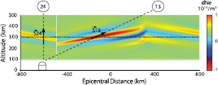
Figure 42. Modeling of Rayleigh wave-induced atmospheric and ionospheric waves 15 min after the Mw 8.3 Tokachi-oki event. Shown are vertical slices of electron density variation dNe. With GPS satellite 13, the integration of the electron density perturbation is constructive in the southwest and destructive in the northeast, while it is fully destructive with satellite 24. From Rolland et al (2011a). Copyright 2011. This material is reproduced with permission of John Wiley & Sons, Inc.
Download figure:
Standard image High-resolution imageThere are other sources of ionospheric disturbances such as auroral, solar activity, and geomagnetic field disturbances unrelated to any event at the surface, which can produce traveling ionospheric disturbances (TIDs) with similar characteristics to those generated by earthquakes (Galvan et al 2012) and can make detection of earthquake-induced TEC anomalies more difficult. Near the equator, post-sunset enhancement of upward plasma drift increases electron density up to altitudes of 500 km, where it creates the equatorial anomaly. After sunset the lower ionosphere rapidly decays creating Rayleigh–Taylor instabilities in the plasma density, which can trigger large variations in the ionosphere called equatorial spread-F (Basu et al 1996). GPS TEC observations have been used to detect and investigate the propagation properties of these plasma depletions (Haase et al 2011). Thus, while these phenomena make the detection of surface sources of ionospheric disturbances more difficult, they are of prime interest to space physics.
6.2.3. Gravity wave methods.
Surface displacements can induce gravity waves that propagate upwards through the atmosphere (Watada 1995). If a volume of air is displaced upwards, buoyancy forces will lead it to sink and oscillate about its neutral buoyancy altitude. It will continue this oscillation about an equilibrium point, generating a gravity wave that can propagate up through the ionosphere. Perturbations at the surface that have periods longer than the time needed for the atmosphere to respond under the restoring force of buoyancy will successfully propagate upwards. This is known as the Brunt-Vaisala frequency and its period is ~5 min at the Earth's surface (Galvan et al 2011). Coupling of surface oscillations with gravity wave modes were observed and modeled using normal mode techniques (Artru et al 2001) for the 2003 Soufrière Hills eruption in Montserrat (Dautermann et al 2009b). Tsunamis can also have periods longer than this frequency and thus excite gravity waves in the atmosphere. Far field gravity waves induced by sea-surface disturbances (tsunamis or underwater landslides) could clearly be seen after the 2006 Kuril Islands, 2009 Samoa, and 2010 Maule tsunamis (Rolland et al 2010, Galvan et al 2011). The vertical propagation speed of an atmospheric gravity wave at these periods is 40–50 m s−1 (Artru et al 2005), so these perturbations should first be observed about 2 h after the onset of the tsunami. The TEC anomalies can be identified by their horizontal propagation speed, which is much slower (200–300 m s−1) than that of the acoustic TID or Rayleigh-wave-induced anomalies and follows the propagation speed of the tsunami itself, which is, much like the Rayleigh waves in the acoustic case, a moving source of gravity waves. However, following the 2011 Mw 9.0 Tohoku-oki, Japan event, which provided dense near-field TEC observations, it was noted that the onset of the gravity-wave-induced TEC anomalies was shorter, at about 30 min after the start of the earthquake, and not the 1.5–2 h predicted by previous theoretical computations (Galvan et al 2012). This is explained as evidence that it might not be necessary for the gravity wave to reach the F layer peak (~300 km altitude) for the TEC disturbance to be measurable. Rather, disturbances at lower altitudes within the E layer and the lower portion of the F layer might be substantial enough to be seen in the TEC observations. This is supported by previous modeling results that showed significant TEC perturbations over a broad area around the F layer peak (Rolland et al 2011b). Through comparisons with tsunami simulations of the event it was convincingly demonstrated that the tsunami itself must be the source of the observed gravity waves (Galvan et al 2012). In light of these observations, ionospheric soundings may be used to monitor tsunamis and issue warnings in advance of their arrival at the coast (Komjathy et al 2012, Occhipinti et al 2013). The long delays between gravity wave generation and the initial perturbation of the ionosphere are a challenge for near-shore monitoring. Furthermore, the relationship between the TEC perturbation amplitude and the tsunami amplitude is modulated by the geomagnetic field and not an immediate assessment of the tsunami size. However, TEC measurements can provide dense coverage of the tsunami area, much denser than other geophysical instruments, and because the slant paths can extend thousands of km away from the observational site, they can provide confirmation long in advance of the incidence of trans-oceanic tsunamis. It is expected that by 2020, there will be over 160 GNSS satellites including those of GPS, European Galileo, Russian GLONASS, Chinese BeiDou, Japanese QZSS, Indian IRNSS, and others broadcasting over 400 signals across the L-band, providing increased ionospheric measurement accuracy with global coverage at a low cost. Utilizing TEC measurements to derive models for the earthquake or tsunami source remains a challenging problem, but is promising, given the success in modeling amplitudes of volcanic and rocket (space shuttle)-generated disturbances (Dautermann et al 2009b, Bowling et al 2013).
There have been suggestions of TEC anomalies occurring before large earthquakes. Precursors to large earthquakes remain elusive in seismology, thus such controversial claims receive widespread attention. Notably Cahyadi and Heki (2013) and Heki and Enomoto (2013) documented TEC observations from several large earthquakes up to and including the Mw 9.0 Tohoku-oki event. After removing the daily TEC trend, they found anomalous increases in TEC up to 40 min before rupture. They claimed that the amplitude of the anomalous precursor scales with the magnitude of the eventual earthquake, such that large earthquakes have significant TEC anomalies before rupture. The claims made in these papers were carefully analyzed and attributed to critical oversimplifications in the processing of the TEC time series (Masci et al 2015). In order to remove the daily TEC signal, a 3rd order polynomial was fit to the daily TEC time series that excluded the 40 min before the event and the hour immediately following the earthquake (Cahyadi and Heki 2013). After removing this polynomial trend, the pre-event anomaly is indeed noticeable. This choice of polynomial fitting appears to bias the residual time series in such a way as to favor artificial pre-seismic signals (Masci et al 2015). After a large ionospheric disturbance such as those produced by a large earthquakes, an ionospheric 'hole' is left behind (Kakinami et al 2012). That is, that portion of the ionosphere is temporarily depleted of free electrons. These holes can persist for many hours. Thus, including post-event data with low TEC in their polynomial fit (Cahyadi and Heki 2013) biased the pre-event data to show an anomalous increase in TEC. It also showed that the flattening in the daily TEC time series was observed during other days without an earthquake and could be easily attributed to normal daily activity levels in the ionosphere (Masci et al 2015). Similar controversies accompanied apparent precursors to other earthquakes, for instance, the 1999 Mw 7.1 Hector Mine earthquake in southern California (Su et al 2013, Masci et al 2014, Su et al 2014). GPS TEC precursors that were claimed to be observed prior to the 2003 Mw 6.6 San Simeon earthquake were shown to be unfounded when systematically analyzed in the context of two continuous years of GPS TEC data for southern California (Dautermann et al 2007). It appears that the pre-seismic ionospheric precursors proposed thus far do not hold up to scrutiny.
7. Climate
7.1. Motivation
The degree and extent of anthropogenic-driven climate change and its mitigation are pressing issues facing the world. The latest report of the Intergovernmental Panel on Climate Change (Stocker et al 2014) presents a mean rate of a global average sea level rise of 1.5–1.9 mm yr−1 from 1901 to 2010, 1.7–2.3 mm yr−1 from 1971 to 2010, and 2.8–3.6 mm yr−1 from 1993 to 2010. Since the 1970s (figure 43), ice mass loss and ocean thermal expansion from warming account for 75% of sea level rise; from 1993 to 2010, global mean sea level rise contributions include 0.8–1.4 mm yr−1 from ocean thermal expansion due to warming, 0.25–0.41 mm yr−1 from the Greenland ice sheet, 0.16–0.38 mm yr−1 from the Antarctic ice sheet, 0.39–1.13 mm yr−1 from other glaciers and ice caps, and a decrease of 0.26–0.49 mm yr−1 from land water storage; the sum of 2.3–3.4 mm yr−1 explains most of the overall estimate of 2.8–3.6 mm yr−1 rise of the global sea level from 1993–2010 (Stocker et al 2014). Estimating sea level rise is complicated by the fact that coastlines are not static over that time period. Land deformation (subsidence, uplift, horizontal) is occurring due to tectonic motion, isostatic adjustment due to long-term glacial retreat, earthquakes, tsunamis, sediment compaction, and anthropogenic sources (water, oil, and mineral extraction). Shorter term and periodic effects such as tsunamis, tides, meterorological sources of waves and storm surge, seasonal and longer term variations in water transport, currents, and salinity superimpose on the global signal to exacerbate the sea level rise. Small amplitude coupled changes become important when attempting to link the ocean tide gauge record to an absolute reference frame and effects from the Earth's tides, the Earth's orientation changes, atmospheric pressure, and ocean loading must be considered. GPS positions and displacements from a global network of tracking stations are 'absolute' with respect to a global terrestrial reference frame, so that direct observations of contemporary vertical land motion (VLM) of coastal areas near traditional tide gauges and 3D GPS displacement on bedrock at the periphery of ice sheets, as well as indirect measurements of glacial isostatic adjustment (GIA) can be used for quantifying absolute sea level rise (note that in sections 7 and 8 we use VLM and land subsidence/uplift interchangeably). As described in this section, GPS geodesy is playing an important role in climate research by providing increasingly long reference time series of precise position and displacement. Precise absolute GPS positions are also used to supplement and calibrate other observational systems including satellite radar altimeters, satellite gravimeters, and tide gauges. GPS geodesy also contributes directly to measuring long-term changes in atmospheric water vapor and temperature through the measurement of atmospheric delays (section 6.1). Observations from land- and satellite-based sensors are used to estimate trends and seasonal variations in atmospheric water vapor and temperature, important benchmarks for the assessment of global climate change.
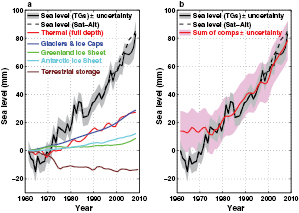
Figure 43. The global sea-level budget from 1961 to 2008. (a) The observed sea level using coastal and island tide gauges (the solid black line with gray shading indicating the estimated uncertainty) and using TOPEX/Poseidon/Jason-1 & 2 satellite altimeter data (dashed black line). (b) The observed sea level and the sum of components. The estimated uncertainties are indicated by the shading. From Church et al (2011). Copyright 2011. This material is reproduced with permission of John Wiley & Sons, Inc.
Download figure:
Standard image High-resolution image7.2. Sea level rise and land subsidence
Populations and infrastructure in coastal regions and island nations are affected by changes in sea level. Rising mean sea level on a global scale is an important metric for climate change, but there is also significant variability at local and regional scales (Cazenave and Nerem 2004). There have been intense discussions on the magnitude of sea level change and its uncertainties, as well as the contributions of a myriad of underlying physical processes (Cazenave and Nerem 2004, Cazenave and Llovel 2010), for example, the enigma posed by the factor of 2 differences in the observed global mean sea level change and the sum of the estimated contributions from each source over the last half of the 20th century (Munk 2002). Advances in satellite geodesy, observations by spaceborne radar altimeters gravimeters and more recently by GPS have narrowed these differences.
Changes in the global sea level relative to the deforming solid Earth are classified according to changes in ocean volume through thermal expansion (referred to as 'steric') and to changes in ocean mass through the melting of land ice (referred to as 'barystatic'). The surface of an ocean of constant density without the effects of tides, currents, winds, and waves, i.e. solely under the influence of the Earth's gravitation and rotation, would closely coincide with the geoid. By definition, the geoid (figure 44) is a gravitational equipotential surface that is oriented everywhere perpendicular to the force of gravity. On land, elevation (topography) is measured with respect to the 'mean sea level' as represented by the geoid; over the oceans 'topography' is obtained by radar altimeters as the difference between the remotely sensed surface and the reference geoid determined by gravity measurements. At the land–ocean interface, the two, in theory, should be equivalent. GPS observations, provided with respect to an Earth-centered, Earth-fixed reference frame (section 2.5.3) and to first order, are independent of gravity. An Earth-centered global oblate ellipsoid rotating with the Earth is defined, which approximates the size and shape of the Earth (geoid), named by convention the World Geodetic System 1984 (section 2.5.3). GPS positions can be expressed in terms of geodetic latitude and longitude and height above this geometric reference ellipsoid. The height of the geoid relative to the reference ellipsoid is called the geoidal undulation and varies by about −105 m to 85 m over the Earth. The undulation at any point on the Earth's surface is related to the direction and intensity of gravity at that point. Thus, a sufficiently detailed and precise global gravimetric model based on land (spirit leveling) and satellite (gravity) observations provides a realization of the geoidal surface and the connection to GPS observations through the geoidal undulation.

Figure 44. Reference surfaces. The ellipsoid is a purely mathematic construct that approximates the Earth's size and shape and is used as a reference for geodetic latitude and longitude (figure 3). The geoid is a physical surface defined by the gravitational field, used as a reference for heights above sea level.
Download figure:
Standard image High-resolution imageSea level has been historically measured using tide gauge data (Douglas 2001). For example, tide gauge data held by the NOAA's National Geophysical Data Center (available from their website) are from 1854, and European observations began at least a century earlier. The use of tide gauges for the study of climate change is problematic because it measures sea level with respect to the solid Earth at the local coastline, which is subject to deformation. In order to be able to predict and mitigate the effects of coastal inundation, it is necessary to consider both rising sea levels and land subsidence, the latter of which may be caused by anthropogenic effects (e.g. the extraction of groundwater, oil, and minerals) and by natural processes such as large subduction zone earthquakes and coastal erosion. For example, a GPS showed that Japanese coastal stations during the 2011 Mw 9.0 Tohoku-oki earthquake subsided by up to a meter (Grapenthin and Freymueller 2011, figure 23). Furthermore, global tide gauge coverage is limited and is sparser in the southern hemisphere. Tide gauge measurements are relative to a fixed point on land, historically surveyed by expensive and cumbersome spirit leveling, and thus must be put into an absolute reference frame in order to provide information on the global trend. Although the selection of appropriate data sets is sometimes subjective, recent analyses of global sea level rise based on tide gauge records indicate an acceleration from 1.5 mm yr−1 prior to 1990 to 3.2 mm yr−1 by about 2005, mostly accounted for by an acceleration in the tropical and southern oceans (Merrifield et al 2009).
Global mean sea level rise determined by satellite radar altimetry observations over the open oceans provides a direct measurement of sea surface (dynamic) topography and does not suffer from the susceptibility of sparse tide gauge measurements to VLM. Furthermore, altimetry can resolve interannual fluctuations due to, for example, El Niño and La Niña events better than tide gauge records, and it also detects significant regional variability (Cazenave and Nerem 2004, Cazenave and Llovel 2010). The first decade of measurements (1993–2003) from TOPEX (Topography Experiment/Poseidon) and Jason satellite altimeters yielded a rate of 2.8 ± 0.4 mm yr−1 of global sea level rise with an increase to 3.1 mm yr−1, if the effects of GIA (section 7.4) are considered, which is significantly higher than the 1–2 mm yr−1 estimated from the 20th century record of tide gauge observations. Adding another four years of measurements from altimetry and the available tide gauge data provided a slightly refined estimate of 2.85 ± 0.35 mm yr−1 for sea level rise, which was less than the value of 3.3 ± 0.4 mm yr−1 derived strictly from altimetry. The components of sea level rise are attributed as follows: 30% to ocean thermal expansion and 55% to land ice melt and mass loss. Total ice mass loss increased to 80% of the total over the last five years of the record, and regional variations due to thermal expansion and changes in ocean heat storage (Cazenave and Llovel 2010).
An important data set for correcting tide gauge records for vertical land motion (VLM) is absolute vertical positions estimated at nearby GPS stations. Local VLM can be as large, or larger, than the sea level rise signal. Attempts to use satellite altimeter measurements to correct tide gauge records have had mixed results (Nerem and Mitchum 2002). It has been argued that assessing accelerations in sea level rise is not limited by vertical land motion; it is only the absolute levels that require a correction (Merrifield et al 2009). However, this assumes that VLM is uniformly linear, and the same assumption needs to be made when using GPS vertical velocities to calibrate historic tide gauge data in the 20th century. Furthermore, one must assume that the velocity at the GPS station is the same as the ground to which the tide gauge is attached, and that the GPS monument is locally stable. The global GPS vertical velocity estimates are significantly more precise than the expected sea level rise signal (1–3 mm yr−1). As described in sections 2.3 and 3, the accuracy of GPS displacement time series is affected by a variety of physical and instrumental offsets, as well as spatial and temporal correlations that need to be taken into account. Nevertheless, time series analyses of thousands of GPS stations indicate that the standard deviation of the vertical velocities over a 10–20 year period are on the order of 0.1–0.3 mm yr−1. As an example, consider the tide gauge record at the pier at the Scripps Institution of Oceanography from 1924 to the present, which shows a rate of sea level change of 2.02 ± 0.25 mm yr−1 (figure 45). The 13 year (2002–2015) GPS vertical velocity estimate of a station within 3.5 km of the pier indicates a significant subsidence of −0.56 ± 0.15 mm yr−1. A study of 28 globally-distributed and globally-referenced GPS vertical time series up to 7 years in length, within 16 km or less from tide gauges with records of ~50–100 years, yields a GIA-corrected (section 7.4) global sea level change average of 1.31 ± 0.30; without the GPS correction the value is 1.83 ± 0.24 mm yr−1, indicating the influence of land subsidence (Wöppelmann et al 2007). In the 20th century, sea level rise is estimated to be composed of about 1 mm/yr from barystatic changes (ice flux) (Mitrovica et al 2006) and about 0.4 mm yr−1 from steric changes (thermal ocean expansion; from 1955–2003 for ocean depths up to 3000 m, Antonov et al 2005). Thus, at least from this study (Wöppelmann et al 2007), after correction for land subsidence from GPS, and taking into account GIA, the sea level enigma posed by Munk (2002) appears to be resolved.

Figure 45. Tide gauge record at Scripps Institution of Oceanography showing a rise of 2.02 ± 0.25 mm yr−1 (95% confidence) based on linear regression, starting in 1924 and extrapolated back to the beginning of the 20th century. Reproduced with permission from the NOAA's Center for Operational Oceanographic Products and Services.
Download figure:
Standard image High-resolution image7.3. Mass balance of the ice sheets
Mass variations in the Earth's ice sheets and the associated sea level rise are a consequence of rising air temperatures and global climate change. A careful combination of a diverse set of satellite data (altimetry, interferometry, and gravimetry) using common geographical regions, time intervals, and models of surface mass balance and glacial isostatic adjustment has provided a definitive estimate of the mass balance of the polar ice sheets.
In the period between 1992 and 2011, the ice sheets of Greenland, East Antarctica, West Antarctica, and the Antarctic Peninsula changed in mass by −142 ± 49,+14 ± 43,−65 ± 26, and −20 ± 14 Gt yr−1, respectively, and contributed, on average, 0.59 ± 0.20 mm yr−1 to the rate of global sea level rise (Shepherd et al 2012). The mass loss is not linear, however. For example, in Greenland the effect of warming increases the volume of lubricating surface meltwater reaching the ice-bedrock interface, which accelerates ice flow and results in more mass loss than expected from melting alone. Ice loss to the ocean exceeding that replaced by annual snowfall would then contribute to sea level rise. In 2006 the Greenland and Antarctic ice sheets experienced an anomalously high combined mass loss of 475 ± 158 Gt yr−1, equivalent to a 1.3 ± 0.4 mm yr−1 sea level rise (Rignot et al 2011). However, since 2006 this rate has accelerated to 273 Gt yr−1, equivalent to 0.75 mm yr−1 of global sea level rise due to high summer melt rates (van den Broeke et al 2009).
Acceleration in ice sheet loss over the last two decades has been quantified at 21.9 ± 1 Gt yr−2 for Greenland and 14.5 ± 2 Gt yr−2 for Antarctica, and 12 ± 6 Gt yr−2 for mountain glaciers and ice caps (Rignot et al 2011). Clearly the effects in Greenland are dominating this acceleration. Ice loss from the Greenland ice sheet over the last two decades are estimated to account for about 0.5 mm yr−1 of a total of 3.2 mm yr−1 of global sea level rise over the last two decades, with a significant portion due to accelerations of glaciers in the southeast and northwest (Velicogna and Wahr 2006, van den Broeke 2009, Khan et al 2014).
Estimation of changes in the vertical (dh/dt, where h is the height above the ellipsoid) from repeated GPS surveys is a critical complement to the satellite remote sensing methods to assess the impact of climate change and climate cycles on ice mass balance, primarily in the Antarctic and Greenland. This is because the altimeter measures only the height of the ice surface; however, because of the isostatic compensation for the mass unloading, the Earth's crust below the ice is uplifting. Therefore the vertical motion measured by variations in position of GPS stations on exposed bedrock are critical to correct for the uplift of the bedrock base of the ice mass. Up to two decades of GPS-derived accelerations in the North Atlantic region indicate accelerating uplift over the past decade, which is modeled as an essentially instantaneous, elastic response to the recent accelerated melting of ice throughout the region (Jiang et al 2010). Accounting for GIA and using an elastic model, they find that by the late 1990s western Greenland's ice loss was accelerating at an average rate of 8.7 ± 3.5 Gt yr−2, whereas the rate for southeastern Greenland, although with a more limited data set, was 12.5 ± 5.5 Gt yr−2.
7.3.1. Variations in the Greenland ice sheet flow rates.
Mass loss from Greenland's ice sheet results from melt runoff (surface and basal) and dynamic thinning due to the speed-up of the glacier flow at its edges along the ocean margins (southwest, west, and northwest), and iceberg calving. In the southwest, mass loss up to 100 km inland is dominated by atmospheric forcing; in the northeast, major marine-terminating outlet glaciers are surrounded by year-round sea ice, which suppresses calving front retreat, and up to 600 km inland ice streams are undergoing dynamic thinning linked to regional warming (Khan et al 2014).
The discovery, through direct GPS position and interferometric satellite radar measurements, that seasonal accelerations of major ice streams and outlet glaciers that drain Greenland (Zwally et al 2002, Joughin et al 2008, Das et al 2008, van de Wal et al 2008) are coupled with the duration and intensity of surface melting, supports the rapid and large-scale dynamic response of ice sheets to climate change. Early studies of seasonal velocities of the major fast-moving Jakobshavn Isbrae (figure 46) ice flow (~2.5 m yr−1 estimate based on ice mass loss from melt as compared to the ~100 m yr−1 observed westward flow to the ocean) in West Greenland using terrestrial survey measurements (EDM and theodolite) and Doppler satellite navigation (the much less accurate predecessor of the GPS) showed no significant variations in seasonal velocities within the uncertainties of the geodetic measurements (Echelmeyer and Harrison 1990). On the other hand, significant seasonal variations in velocity ranging from 35–40 cm d−1 (127.8–146.0 m yr−1) in the summer to 27–28 cm d−1 (98.6–102.2 m yr−1) in the winter were observed with a GPS (Zwally et al 2002). These observations undertaken in western-central Greenland from 1996–9 monitored the horizontal motion of a single 4 m pole embedded to a depth of 2 m in the ice near the equilibrium line (the point at which accumulation and ablation are in balance). Although sparse, this dataset supports the hypothesis that glacial sliding is enhanced by rapid migration of surface meltwater to the ice-bedrock interface (Zwally et al 2002). The GPS displacements were analyzed in combination with three years of RADARSAT measurements with 24 d repeat cycles, and indicated widespread seasonal accelerations of 50–100% of the slow-moving ice sheet, but only <15% acceleration of the faster-moving outlet glaciers that discharge ice directly into the ocean (Joughin et al 2008).
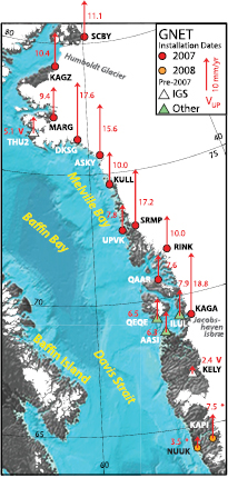
Figure 46. Observed cGPS vertical velocities in west and northwest Greenland. One sigma standard errors (66.7% confidence) are 1 mm yr−1 or less (not shown). Reproduced with permission from Bevis et al (2012). Copyright 2012 U. S. National Academy of Sciences.
Download figure:
Standard image High-resolution imageLocal GPS surveys, seismic measurements, and water level sensor observations of the rapid drainage of two large supraglacial lakes on Greenland's west margin, down nearly a km to the ice sheet bed, were used to study the process by which surface meltwater reaches the base of the ice sheet, creating a mechanism for the rapid response of ice flow to climate change (Das et al 2008). Drainage over less than 2 h coincided with increased seismicity, transient acceleration, ice-sheet uplift, and horizontal displacement, while subsidence and deceleration occurred over the subsequent 24 h, indicating that the integrated effect of multiple lake drainages could explain the observed net regional summer ice speed-up. Using a 250 km transect of continuous GPS stations from the coast inland, large and rapid velocity changes were observed in the region of ice ablation in western Greenland (van de Wal et al 2008). A single-frequency GPS receiver measured ice velocity at a resolution of about 1 d, recording changes of up to 30% over a weekly period, significantly greater than earlier studies. A study of the northeast Greenland ice stream (Khan et al 2014), which extends more than 600 km inland and drains more than 16% of the total ice sheet, demonstrated accelerated mass loss linked to recent regional warming, indicating additional mass loss for the calculations of future global sea-level rise.
Time series of GPS positions on bedrock stations along Greenland's west coast showed an annual oscillation superimposed on a sustained upward trend in the vertical direction (Bevis et al 2012) (figure 47). The oscillation is driven by the Earth's elastic response to seasonal variations in ice mass and air mass (atmospheric pressure) and the vertical trend is much higher than predicted rates of long-term viscoelastic compensation by glacial isostatic adjustment in the mantle (section 7.4), implying that uplift is dominated by the solid Earth's instantaneous elastic response to contemporary losses in ice mass. The GPS-observed accelerated uplift at the front of the glacier during the period 2008–13 can only be due to an instantaneous response, indicating that mass loss has accelerated in the past decade (Bevis et al 2012), confirming the results of satellite- and airborne-based elevation data (Khan et al 2014).

Figure 47. (A) Vertical displacement time series at eight GPS stations (blue dots) on bedrock on the west coast of Greenland (figure 46), and model trajectory (red) curves composed of an annual oscillation, plus a multiyear trend. (B) Fit trajectory model at station HEL2. Reproduced with permission from Bevis et al (2012). Copyright 2012 U. S. National Academy of Sciences.
Download figure:
Standard image High-resolution image7.3.2. Variations in the flow rate of the Antarctic ice sheet.
Glaciers in Antarctica drain more than 30% of the continent, funneling ice through fast-flowing and highly-dynamic ice streams. GPS displacement observations of markers implanted in glaciers have been used to detect and quantify temporal variations in ice flow, helping to understand the dynamics of the Antarctic ice sheet and consequently the contribution of Antarctic ice loss to global sea level change. One important question is how the ice streams move on short time scales, and a surprising discovery showed a stick-slip motion on the Whillans ice stream (figure 48), West Antarctica. Five GPS receivers surveyed 29 stations on the ice plain on its downstream side and the nearby Ross ice shelf (figure 48) over a two week period in early 1999, with observations at each location ranging from a few h to 2 d (Bindschadler et al 2003). Variations in positions estimated every 5 min using the precise point positioning approach and relative network positioning between pairs of stations (section 2.4.1) occurred as brief episodes of rapid horizontal slip of durations of 10–30 min at rates up to about 1 m h−1, more than 30 times faster than the already high velocity of the ice stream feeding the ice plain. These significant periods of acceleration were separated by 6–18 h of little to no motion. Using displacements from triplets of stations to reduce asynchronous slip across the ice plain, the mean speed of propagation was approximately 88 m s−1, but with a high uncertainty. The stick-slip motion is thought to be controlled by oceanic tidal oscillations of about 1 m. During a spring-tide period, rapid motions regularly occur near high tide and during falling tide. The motion was modeled, using the GPS-derived speed of the ice stream, as an episodically slipping friction-locked fault bottoming at the base of the ice surface, such that tidal oscillations provided the resistance that controls the timing of slip events. Slip events were explained by the release of stored elastic strain that relieved the subglacial shear stress, followed by a stick period in which additional elastic strain was stored before the next slip event could take place. The study demonstrated rapid changes of speed and its extreme sensitivity to subglacial conditions and variations in sea level (Bindschadler et al 2003).
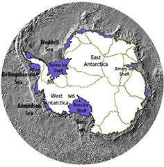
Figure 48. Antarctic ice streams and ice shelves. Together the ice streams drain more than 1/3 of the area of continental Antarctica, funneling the ice via a network of ice streams through narrow exit gates (Rignot et al 2011). Copyright 2011, RIS: Rutford Ice Stream; WIS: Whillans Ice Stream.
Download figure:
Standard image High-resolution imageDual-frequency GPS observations have been used in West Antarctica to measure velocity variations associated with tides. Observations of the locations of 2 m snow driven poles at 60 s intervals over a 24 d period in late 2000 were used to detect inline horizontal velocity fluctuations on the order of 0.7 m d−1. This is a factor of 3 in flow speed (the mean flow speed is about 1.2 m d−1) over the course of the approximately 24 h tidal cycle (Anandakrishnan et al 2003). This effect was most pronounced at the grounding line (the interface between the floating and the grounded parts of the ice), with significant crossline variations. As in an earlier study (Bindschadler et al 2003), the diurnal velocity fluctuations appear to be driven by the tide beneath the Ross ice shelf (figure 48), where the ice stream speeds up during the falling tide and slows during the rising tide.
Correlations with additional tidal frequencies were observed with continuous relative GPS positions of five stations on the Rutford Ice Stream (figure 48), West Antarctica, which were estimated over a seven week period commencing in late December 2003 (Gudmundsson 2006). One site was on a floating ice shelf some 20 km downstream of the grounding line and the other four locations were along the central flow line extending 40 km upstream of the grounding line. The observations revealed variations in flow speeds in two week cycles with about 20% peak-to-peak amplitude due to tidal forcing. Two years of GPS data, collected ~40 km upstream of the grounding line, recorded tidal modulation of ice flow at semidiurnal, diurnal, two-weekly, semi-annual, and annual ocean tidal frequencies (Murray et al 2007). Precise point positions (section 2.4.2) estimated every 5 min over a 750 d period, with a precision (95%) confidence of 2–3 cm horizontally and 5 cm in the vertical, show deviations from the average downstream flow of about 20%, with amplitudes of about 20 cm. Long-period forcing is most pronounced and could provide a feedback loop between rising sea levels and increased ice stream velocity (Murray et al 2007).
Interesting variations occur in East Antarctica, where overall ice velocities appear to be decreasing rather than increasing. A long-term re-analysis of variations in velocity on the northern Amery ice shelf (figure 48) in East Antarctica from 1968–1999 was carried out using triangulation, trilateration, and GPS surveys of poles embedded in the ice. The results suggest a statistically significant slowdown of the ice of about 2.2 m yr−1 or about 0.6% deviation from the long-term centerline velocity (King et al 2007), and provide a baseline for future studies. Iceberg calving on the Amery ice shelf with a dense network of GPS stations, using instantaneous positioning (section 2.4) at a 2 Hz sampling rate, and seismometers deployed over three consecutive annual field seasons around the tip of a propagating rift in the ice, confirmed the episodic behavior of the ice motion linked to the stick slip behavior observed in other regions of Antarctica described above, in this case consisting of several hourly bursts with a recurrence time of several weeks (Bassis et al 2007).
In summary, well-sampled GPS-derived horizontal velocities have revealed Antarctic ice flow accelerations on scales from sub-diurnal to annual, which must be considered when using these data to confirm mass balance estimates determined from satellite observations. They are also important for modeling the process in order to move to predictive estimates of the future evolution of ice sheets and mass balance and sea level rise tied to climate change.
7.3.3. Calibration of satellite altimetry.
Although precise GPS positioning has made direct and significant contributions to climate research in terms of variations in the cryosphere and sea level rise, the difficulties in carrying out land-based observations in these environments are considerable, and much research has depended on remote sensing. Direct GPS ground observations have been used to calibrate satellite-based remote sensing instruments including satellite radar altimeters over Antarctica (Fricker et al 1998, Siegfried et al 2014) and satellite radar interferometry over Greenland glaciers (Mohr et al 1998). NASA's Ice, Cloud, and Land Elevation Satellite (ICESat) altimeter was validated using dense kinematic GPS observations in central Greenland (Siegfried et al 2011) and on the Salar de Uyuni in Bolivia, one of the flattest large natural surfaces, revealing significant biases within the ICESat mission, which propagated into ice-shelf mass balance estimates over West Antarctica (Borsa et al 2014a). Ground GPS and leveling measurements were used to assess the accuracy of a satellite altimeter-based digital elevation model for Antarctica (Bamber 1994). Furthermore, in situ GPS observations of vertical movement were used to cross-calibrate and bridge temporal gaps between the Ice, Cloud, and Land Elevation Satellite (ICESat) and Cryosat-2 missions to evaluate the ability of Cryosat-2 altimetry to measure dynamic changes on the ice sheets (Siegfried et al 2014). A GPS has also been used to provide ground truth for improving the accuracy of Antarctic ocean tide models (e.g. Padman et al 2003, King and Padman 2005) by minimizing unwanted signals from floating ice elevation and space-borne, time-variable gravity measurements such as GRACE (NASA's Gravity Recovery and Climate Experiment).
7.4. Glacial isostatic adjustment
The GPS plays an important role in quantifying glacial isostatic adjustment (GIA), also referred to as postglacial rebound (PGR) (King et al 2010). GIA is one of the biggest sources of error in contemporary ice sheet mass balance calculations using gravity missions (GRACE) for the assessment of variations in mass loss and their impact on sea level rise due to climate change (Shepherd et al 2012). GIA is the viscous response of the Earth to deglaciation from the Last Glacial Maximum at 26 kyr BP to about 4 kyr BP. GIA models are a function of spatio-temporal changes in the thickness of the ice sheet (glaciation history), the viscosity of the mantle as a function of depth, the thickness of the elastic lithosphere, and the lateral homogeneity of the viscoelastic structure (Argus et al 2014a).
It is necessary to distinguish the contribution of vertical uplift due to long-term GIA from the vertical trend due to the solid Earth's instantaneous elastic response to contemporary losses in ice mass. GPS observations provide constraints on these rates, and also help to understand the effects of seasonal variations in ice mass and air mass (atmospheric pressure) (Bevis et al 2009, 2012). Estimates of GIA uplift derived from the radiocarbon dating of marine terraces that indicate sea level changes and estimates of ice thickness change during the deglaciation of Antarctica significantly differ from present-day direct GPS measurements of vertical deformation. Although satellite measurements of time-dependent gravity through the GRACE mission provide an unprecedented measure of total mass change over ice sheets, in order to extract the contribution of ice mass change, correction for the gravitational signature of mass movement in the mantle due to GIA occurring since the last glaciation period is required.
GIA has been shown to be the most significant component of vertical crustal deformation in the polar regions. Since 1993, continuous GPS networks in Fennoscandia (Johansson et al 2002, Milne et al 2004) spanning the region of uplift due to ice mass loss in the Late Pleistocene have shown rates of up to 11.2 ± 0.2 mm yr−1. The pattern and amplitude of GPS velocities show a broad ellipsoidal uplift dome with a major axis oriented roughly southwest to northeast (Milne et al 2001). GPS vertical velocities were found to be consistent with a theoretical GIA model for location and mass of ice removed, which satisfies independent geologic constraints from ancient shorelines and bounds the average viscosity in the upper mantle to the range of 5 × 10²⁰–1 × 10²¹ P · s and the elastic thickness of the lithosphere to 90–170 km. (The GPS observations were also used to correct tide gauge records to determine a regional sea level rise of 2.16 ± 3 mm yr−1). It is interesting to note that inland stations have higher vertical velocity errors compared to coastal areas due to inland snow accumulation on the GPS antennas. Other regions that exhibit significant GIA effects include the broader region of northern Europe, Siberia, North America, Antarctica, and parts of Patagonia in the southern hemisphere. GIA effects, which cover most of the area of Canada and the United States, have been studied extensively to understand the physical processes in the mantle and crust related to mantle convection, plate tectonics, and the thermal evolution of the Earth. Besides sea level rise and climate studies, GIA also complicates studies of crustal deformation at plate boundaries, e.g. the North America/Pacific plate boundary on the West Coast of the United States), which rely on the rigidity of plate interiors as a reference, in this case, a 'stable' North America plate. A study of the North America plate interior based on the motion of hundreds of sGPS stations found that surface deformation was best fit by a model that includes the rigid rotation of North America with respect to the International Terrestrial Reference Frame (ITRF2000, section 2.5.3) and a component of strain qualitatively consistent with that expected from GIA (Calais et al 2006). After correcting for the plate motion, residual horizontal velocities show a north-to-south deformation gradient of ~1 mm yr−1, mostly localized between 1000 and 2200 km from the GIA center, corresponding to strain rates of about 10−9 yr−1.
In the combined analysis of satellite altimetry, interferometry, and gravimetry data sets that led to revisions in earlier estimates (Shepherd and Wingham 2007) of mass change and associated sea level rise, it was necessary to correct for GIA (Shepherd et al 2012). In Antarctica, extensive GPS observations at up to about 50 Antarctic bedrock stations and gravity measurements from the GRACE mission suggest that uplift from GIA models may have been overestimated by about 5 mm yr−1, and that previous secular Antarctic ice mass loss estimates are systematically biased, mainly too high (Bevis et al 2009, Thomas et al 2011). Subsequently, a GIA correction was applied to the GRACE data from 2002 to 2010, which resulted in an Antarctic ice-mass change of −69 ± 18 Gt yr−1 corresponding to 0.19 ± 0.05 mm yr−1 of sea-level rise (King et al 2012), significantly lower than earlier estimates. The corrected data were able to resolve ice mass loss in 26 independent drainage basins; accelerations were found to be concentrated in basins along the Amundsen Sea coast (figure 48), while outside this region West Antarctica was nearly in balance and East Antarctica is gaining substantial mass (King et al 2012).
Several GIA models have been produced that impact the study of sea level rise. The models provide three highly correlated parameters, the thickness of the ice sheet as a function of location and time (the glaciation history), the viscosity of the mantle as a function of depth, and the thickness of the elastic lithosphere (Argus et al 2014a). GIA models ICE-5G (VM2) (Peltier 2004) and IJ05 (Ivins and James 2005, Simon et al 2010) are based on different ice histories and Earth models, and some have been updated for the effects of regional ocean loading (Simon et al 2010). Consideration of the GPS uplift results has led to the development of new GIA models (e.g. Whitehouse et al 2012a, 2012b, Argus et al 2014a) in an effort to improve the Antarctic mass-balance estimates (Shepherd et al 2012, King et al 2012). A new GIA model for Antarctica developed to address systematic over-predictions of uplift rates (Whitehouse et al 2012a, 2012b) improved the fit to both the ICE-5G v1.2 and IJ05 ice models. Uncertainties were assigned to the GIA uplift rate predictions, taking into account uncertainties in both the deglaciation history and the modeled Earth viscosity structure. Uplift rates from 42 GPS bedrock stations in Antarctica, supplemented by available ice thickness changes from exposure-age dating, Holocene relative sea level histories, and the age of the onset of marine sedimentation along the Antarctic shelf from radiocarbon dating were used to develop a new GIA model, ICE-6G_C (VM5a) (Argus et al 2014a) (figure 49). The different GIA models provide varying estimates of the overall contribution of Antarctica ice loss to global sea level rise since the Last Glacial Maximum (26 kyr BP); 8 m from the W12 model (Whitehouse et al 2012a), 7.5 m in the IJ05 R2 model (Ivins et al 2013), and 13.6 m in the ICE-6G_C model (Argus et al 2014a). The higher estimate is attributed to a factor of 2 lower upper-mantle viscosity for the ICE-6G_C model (5 × 10²⁰ Pa s). Furthermore, the ICE-6G_C model fits GPS-derived horizontal velocity values where significant (up to 2 mm yr−1), thus not requiring lateral variations in mantle viscosity. The models also differ in whether or not there is any ice gain in the East Antarctica interior (no gain for the ICE-6G_C model).
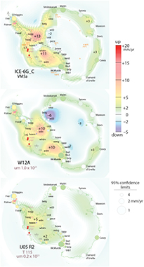
Figure 49. Estimates of uplift at GPS stations (circles) are compared with the predictions of postglacial rebound models (top) ICE 6G C (VM5a), (middle) W12A (Whitehouse et al 2012b), and (bottom) IJ05 R2 (Ivins et al 2013). The colors of the circles indicate the vertical rate of motion estimated by a GPS. The larger the circle, the more certain the estimate (95% confidence). Reproduced with permission from figure 6 in Argus et al (2014a). Copyright 2014. The Royal Astronomical Society.
Download figure:
Standard image High-resolution image7.5. Long-term atmospheric variations relating to climate change
The long-term upward trend in tropospheric temperature since industrialization due to increased anthropogenic CO2 emissions (consistent with radiative effects) should be accompanied by a positive trend in absolute atmospheric water vapor content, assuming moist dynamics would require relative humidity to remain approximately the same. This in turn would enhance through a feedback mechanisms the atmospheric greenhouse effect, rainfall extremes, and changes in the height of the tropopause (Sherwood et al 2010). Strong positive feedback on global warming will result from a water vapor increase unless relative humidity were to decrease rapidly as the climate warms (Sherwood et al 2010). However, significant trends in tropospheric relative humidity at large spatial scales have not been observed, with the exception of near-surface air over land, where the relative humidity has decreased in recent years (Stocker et al 2014). Discerning the long-term trend is complicated by global and regional episodic, short-period, and seasonal variations in tropospheric temperature such as the El Niño–Southern Oscillation (ENSO), volcanic activity, and solar variability. Trends in long-term GPS surface observations of tropospheric delay (6.1.2), supplemented by in situ pressure and temperature readings, may be related to variations in atmospheric water vapor content through precipitable water vapor (section 6.1.3). Long-term GPS radio occultation observations of time delay of the occulted signal's phase traversing the atmosphere (Ware et al 1996, Sokolovskiy 2001, Steiner et al 2011) provide estimates of atmospheric refractivity, from which changes in global atmospheric temperature can be derived in the dry atmosphere (middle-upper troposphere and stratosphere).
7.5.1. Surface GPS measurements.
Increasingly long land-based time series of zenith tropospheric delays and integrated precipitable water (sections 6.1.2 and 6.1.3) from GPS monitoring at hundreds of global tracking stations (Jin et al 2007, Wang and Zhang 2008) are becoming an important climatological data set as a benchmark for discerning trends and periodic variations in atmospheric water vapor (humidity). The GPS data complement water vapor observations from radiosondes, radiometers, satellite missions, and surface (land and sea) observations. The GPS has the advantage of providing an absolute estimate of water vapor with respect to the terrestrial reference frame (which is used to calibrate other instruments such as water vapor radiometers) unaffected by cloud and precipitation (Duan et al 1996). However, unlike other methods such as radiosondes, which provide profiles along the entire atmospheric column above the launch site, the GPS only provides the total zenith delay and integrated precipitable water vapor content. On the other hand, radiosondes typically only sample twice per day, while the GPS samples continuously. In fact, the GPS has been used to calibrate the radiosonde record by detecting time-dependent storage errors and other systematic errors in the two most common radiosondes by comparing the time series of monthly mean PW differences. The radiosonde errors, if not corrected, would have a significant impact on the long-term trend estimate or water vapor (Wang and Zhang 2008).
Two-hourly GPS zenith total delay estimates from a global network of 150 GPS stations of the IGS (section 2.1), for the period 1994–2006, revealed a mean trend of 1.5 mm yr−1, with increases in the Northern Hemisphere, decreases in most parts of the Southern Hemisphere, and increases in Antarctica (Jin et al 2007). Annual variations ranged from 25 to 75 mm with a mean amplitude of about 50 mm, with larger amplitudes at coastal stations. A trend of 1.5 mm yr−1 in ZWD (Jin et al 2007) corresponds to about 0.23 mm PW/year or 2.3 mm PW/decade, which is greater than the predicted value from some climate models. This has not yet been unambiguously discerned in the long-term NOAA's GPS-derived PW time series at mid-latitudes across the continental US, according to its former program manager Seth Gutman. However, the length and density of land-based GPS observations is increasing, in particular in Europe, Japan, China, South Africa, and the United States, with regional efforts providing station spacing of 30–40 km, about the wavelength of significant troposphere variations (Williams et al 1998), where long-term changes in meso-beta (over 20–200 km) and meso-gamma (2–20 km) variability may be observable.
An outstanding question in climate studies is the interplay between variations of atmospheric water vapor and temperature. Above 0 °C the water-holding capacity of the atmosphere increases by about 7% for every 1 °C rise in temperature, as determined by the Clausius–Clapeyron equation, which relates saturation water vapor pressure  to temperature
  (Sherwood et al 2010)
where  is the gas constant for water (461.5 J (kg·K)−1) and
  is the latent heat of vaporization (over ice surfaces it is 2.83 × 10⁶ J kg−1; over water 2.50 × 10⁶ J kg−1). The relative humidity is given by
  , where e is the water vapor pressure, which is also related to the vapor density
  , through
By definition, precipitable water is given by
where  is the density of water (see also section 6.1.3 for approximate expressions used for GPS meteorology). Therefore, for a completely saturated column of air, the maximum precipitable water vapor is related to the air temperature in the following manner
PW derived from a decade of GPS troposphere delays during the period of 1994–2004 and surface meteorological data were compared with modeled  assuming water vapor saturation and using ECMWF temperature profiles during that period. In high latitude regions, there was a high correlation between the two, indicating that the PW follows the expected Clausius–Clapeyron equation (128) and may be expected to increase with a warming climate; for lower latitudes, the water vapor content was weakly correlated with temperature, and there was a slight negative correlation in the tropics (Vey et al 2009). There were only limited sites where this could be investigated because at others the GPS-derived PW estimates were found to be sensitive to artifacts in the troposphere delay time series due to changes in antenna type and antenna cover, as well as the changes in the elevation cutoff angles at about the 1 mm level in PW. However, even for the high latitude sites where a trend might be expected, the uncertainties in PW estimates precluded the observation of a significant linear trend. For example, trends at European stations were at the level of about 0.2 mm yr−1, but with a similar uncertainty. It is clear that longer and well-understood PW data sets, in terms of accuracy and precision, will be required to serve as effective benchmarks for assessing variations in atmospheric water vapor for climate change studies.
7.5.2. Satellite-based radio occultations.
Radio occultation data are available from several satellite missions, such as Satélite de Aplicaciones Científicas-C (SAC-C), the GPS/Meteorology (GPS/Met) proof-of-concept mission CHAllenging Minisatellite Payload for geoscientific research (CHAMP), the US/Taiwan constellation of six mini-satellites COSMIC/FORMOSAT3 (Constellation Observing System for Meteorology, Ionosphere, and Climate/Formosa Satellite Mission 3), GRACE, and the EUMETSAT METOP-1 and -2 missions (Anthes 2011). The basic observations are the dual-frequency GPS phase and amplitude measurements that have been delayed as the signal traverses the entire dispersive and neutral atmosphere. The change in phase (Doppler shift) is used to derive the refractive bending, from which atmospheric variables including refractivity, geopotential height, and temperature can be estimated (figure 50). The accuracy of temperature change thought to be required for detecting climate change is 0.5 K and 0.04 K/decade (Ohring et al 2005, Anthes et al 2008). Refractivity  can be expressed (see also section 6.1.2) as
where P and e are the pressure and water vapor pressure, respectively, in hPa, 77.6 and 3.73 × 10⁵ are the empirically determined constants with units K/hPa and K2/hPa, ne is the electron density (in number of electrons per cubic meter) and f is the GPS frequency. The ionospheric effects are removed using an ionospheric correction to the derived bending angle. Because of the ambiguity between determining both the temperature and water vapor from a single refractivity measurement, a 1D variational (1DVAR) technique is used to retrieve temperature, humidity, and sea-level pressure (Poli et al 2002).
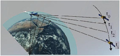
Figure 50. Schematic of the GPS radio occultation method. The basic observations are dual-frequency GPS phase measurements that have been delayed as the signal traverses the entire dispersive and neutral atmosphere. The platform for collecting observation is either airborne (as shown here) or satellite-borne as part of the COSMIC mission, for example. The structure of the atmosphere can be inferred from precise measurements of the amplitude and Doppler shift of the radio waves. From Haase et al (2014). Copyright 2014. This material is reproduced with permission of John Wiley & Sons, Inc.
Download figure:
Standard image High-resolution imageMonthly mean radio occultation measurements from CHAMP and COSMIC missions were used to assess zonal-mean temperature climatologies within 50°N to 50°S in the upper troposphere and lower stratosphere between 300–30 hPa (~9–25 km) (Steiner et al 2009). At lower altitudes, the effects of atmospheric water vapor are problematic for climate studies, while at higher altitudes, residual ionospheric and GPS orbital errors are problematic (Anthes et al 2008). The temperature record was not sufficiently long to distinguish a trend given the interannual variability associated with El Niño and other effects, although a significant cooling trend in the tropical lower stratosphere was found (Steiner et al 2009). An encouraging sign, as the climatological record has been extended, is that temperature results from four different satellite missions to date agree within <0.1K between 8 and 35 km altitude, and monthly mean tropical tropopause temperatures show a consistency of <0.2–0.5K (Foelsche et al 2009). A comprehensive study of upper troposphere/lower stratosphere radio occultation observations, collected by several satellite missions from 1995–2010, which investigated climate change pattern in refractivity, geopotential height, and temperature fields compared to predictions based on several global climate models (GCM) (Lackner et al 2011) did not discern a global pattern. An 'emerging climate change signal' was found only in the geopotential height (the height above the mean sea level of a pressure level), which reflects overall tropospheric warming, at a 90% confidence level with low confidence for large-scale temperature changes and no change in refractivity at the 90% level. At smaller scales, temperature changes are detected at a 95% confidence level, but appear stronger than GCM-projected trends. Because of the lack of any significant natural changes in climate forcing such as volcanic eruptions or solar variability during the time period of observations, the small but significant detected change is suggested to be due to anthropogenic forcing (Lackner et al 2011). Other authors found variations in the geopotential height record at 200 hPa based on radio occultation data over a shorter record compiled from 2002 to 2008, which showed good agreement in the tropics in terms of annual mean and interannual variability with the Coupled Model Inter-Comparison Project phase 5 (CMIP5, Taylor et al 2012), but poor agreement elsewhere. In terms of seasonal variability, the models predicted larger than expected signatures in the northern mid-latitude land areas and the Southern Ocean, but less than expected over the tropics and Antarctica (Ao et al 2015). It is clear that longer radio occultation data sets will be required to serve as effective benchmarks for assessing climate change models.
8. Environmental monitoring
8.1. Motivation
As climate change is affecting the Earth's environment, the GPS is playing an important role in monitoring possibly geographically shifting physical changes that may impact society such as scarce water resources, agricultural productivity to feed growing populations, increased flooding hazards, and more extreme weather, all of which may have serious political ramifications. In this section we focus on regional land subsidence and innovative ways to monitor vegetation growth, soil moisture, and snow cover. In both cases, we describe how these processes affect GPS signals first as 'noise' in precise positioning, and in turn how the GPS can be used to derive information on the processes themselves. We have already described the role of land subsidence in the study of volcanic deformation (section 5.4), in correcting for sea level rise based on tide gauge measurements (section 7.2), and in validating models of glacial isostatic rebound (section 7.4).
8.2. Land subsidence as noise
Land subsidence (or uplift), also referred to as vertical land motion (VLM), is driven by natural or anthropogenic sources from local to global spatial scales, and temporal scales ranging from seconds (e.g. earthquakes) to millions of years (e.g. orogeny). Natural processes include earthquakes that cause episodic coseismic and postseismic deformation (this is an important factor in assessing sea level rise and its climatology), tsunamis, volcanoes, precipitation (rain and snow), drought, flooding, erosion, glacial isostatic adjustment, and sediment compaction. Anthropogenic sources may include filling and depletion of aquifers through groundwater extraction (Galloway and Burbey 2011), oil and mineral extraction (most recently fracking, also a problem because of induced seismicity), hydrothermal power generation (Mossop and Segall 1997, Glowacka et al 2005), and environmental changes such as dams, water projects, and other large infrastructure projects. Although spirit leveling had been the preferred method to accurately measure VLM, in the last two decades it has been primarily done through precise GPS positioning and InSAR. The GPS has the advantage of providing absolute measurements of VLM, with respect to a global terrestrial reference frame (section 2.5.3). Subsidence or uplift in the vertical direction may also be accompanied by smaller horizontal motions due to the ground tilting towards or away from the center of subsidence or uplift, respectively (King et al 2007, Wahr et al 2013). At local scales, land subsidence can have significant seasonal dependence as well as longer-term secular trends. In this section, we discuss VLM as noise that obscures other physical processes of interest. In the next section, we present two examples where the VLM signal is of direct interest.
For measuring crustal deformation, GPS observations and networks are designed so that non-tectonic signatures are minimized by careful site selection that avoid areas known to be affected by hydrological and other changes. In addition, GPS monuments are designed for maximum stability so that the measured motion of a station is representative of the tectonic regime under investigation (figure 7). This is not always possible or effective. For example, seismically-active southern California includes extensive areas of tectonic uplift. However, measuring that is complicated by subsidence, especially in the Los Angeles basin, the Santa Ana basin, the San Gabriel Valley, and the San Bernardino Valley (King et al 2007, figure 51). The San Andreas fault trends generally to the northwest (~45°); north of Los Angeles, a section of the fault referred to as the big bend is oriented more north northwesterly, causing a contraction of the Los Angeles basin and slip taken up by some combination of thrust and northeast-trending strike slip faulting (Walls et al 1998). The nature and rate of the contraction of the basin is important for assessing seismic risk, especially after the destructive 1994 Mw 6.7 Northridge earthquake, which occurred on a blind thrust fault (a blind thrust is one that does not reach the surface). Complicating the problem of identifying other blind thrusts is the effect of groundwater pumping and oil extraction, which affect about 50% of the GPS tracking stations in the region, and which interfere with measuring tectonic signals from thrust faulting. The rate of contraction was estimated to be 6 mm yr−1 from GPS measurements (Argus et al 1999), without consideration of anthropogenic subsidence and 4.5 mm yr−1 from GPS and InSAR measurements (Bawden et al 2001) after modeling subsidence and the related horizontal motions at the edges of subsiding aquifers. An analysis of GPS daily coordinate time series in southern California noted anomalous signatures at a single station in the San Gabriel Valley starting in 2005 (King et al 2007). However, it was not a transient signal of tectonic interest, rather the anomaly was attributed to an extremely heavy rainy season with up to 16 m of groundwater changes in wells. On closer examination, a larger area was affected sampled by ten other GPS stations. The single station had an uplift of about 47 mm with the other stations moving away from the area of uplift in the horizontal components by about 10 mm. These motions were confirmed by InSAR measurements (figure 51). The same event manifested itself in small pockets of motion in the nearby San Bernardino Valley; the difference in the rates of uplift were attributed to groundwater recharge in the widespread unconsolidated sediments in the San Gabriel and San Bernardino Valleys. Subsidence in the Las Vegas Valley, Nevada since 1935 was investigated using GPS and InSAR data in the period 1991–2000, and compared to previous spirit leveling measurements (Bell et al 2002, 2008). The sites were located in a 1300 km2 alluvial valley, and since the 1960s groundwater withdrawals, which have provided the needs of a growing population and rapid development, have exceeded natural recharge.

Figure 51. Continuous GPS horizontal displacements (arrows) in the period 2005.0–2005.4 in the San Gabriel Valley, southern California, caused by aquifer recharge due to heavy rain. The station LONG had an uplift of 47 mm. The signal is the cumulative discrepancy between the post-2005.0 trend and the extrapolation of the trend and annual oscillation established by data before 2005.0. The colors denote the January 2005 to July 2005 InSAR interferogram converted to vertical deformation. Note that the anomalous non-tectonic horizontal displacements bias crustal deformation estimates in this region. From King et al (2007). Copyright 2007. This material is reproduced with permission of John Wiley & Sons, Inc.
Download figure:
Standard image High-resolution image8.3. Land subsidence as signal
8.3.1. Preserving the city of Venice, Italy.
Tidal, storm, wind and atmospheric pressure-induced seasonal flooding coupled with natural and anthropogenic land subsidence have been perennial problems in the city of Venice, Italy, possibly contributing to the dwindling population. In addition to the typical devastation associated with flooding, the primary damage to Venice's art and architecture results from seawater impregnating and destroying building materials, such as limestone and marble (Camuffo and Sturaro 2004). Local (relative) sea level rise has resulted in increased frequency and severity of flooding. In the 21st century, the Venice Lagoon has seen several severe high water events ('acqua alta'), where 50% or more of the city of Venice is affected, ranging from 1.56 m above the mean sea level in 2008 and 1.43 m in 2013. The most severe event to date was 1.94 m in 1966. Based on geology and excavated artefacts, the rate of the local sea level rise has increased from about 0.7 mm yr−1 prior to human habitation (~5th century BCE) to 1.3 mm yr−1 by the late 19th century. Modernization in the 20th century accompanied by groundwater pumping seriously accelerated the subsidence (Gatto and Carbognin 1981). In the 20th century, the Venice tide gauge recorded a sea level rise of 23 cm (figure 52), consisting of ~12 cm land subsidence (3–4 cm from natural causes including tectonic motion, soil compaction, and sediment load, and 6–8 cm from anthropogenic causes due to groundwater extraction), and ~11 cm from the global mean sea level rise in the upper Adriatic. The natural subsidence is thought to be composed of a long-term component (106 yr) due to the retreat of the Adriatic plate subducting beneath the Apennines (Carminati et al 2003) and a short-term component (103–104 yr) controlled by climatic changes through glaciation cycles (Carminati and Di Donato 1999). To protect the city, littorals and lagoon from the flooding, cessation of groundwater pumping was initiated in the 1970s, groynes were built, and wetland reconstruction raised the banks of the city by 10–20 cm. In addition, the controversial (Bras et al 2002, Pirazzoli 2002) MOSE (MOdulo Sperimentale Elettromeccanico, Experimental Electromechanical Module) project (Gentilomo and Cecconi 1997) was started in 2003 and is scheduled to be completed in 2017. MOSE consists of 78 massive steel gates across the three lagoon inlets fixed to massive concrete bases dug into the sea bed. The plan is to raise the flood gates when the tides reach a pre-determined critical height of 1.1 m. Exceeding this height is expected to occur up to five times a year, and is based on the expected barystatic sea level rise, but assumes that vertical land motion (the 'sinking' of Venice) has been mitigated through the regulation of fluid extraction, based on geodetic studies in the last decade of the 20th century (Tosi et al 2002, Teatini et al 2007) and in the first decade thereafter (Teatini et al 2012a). The MOSE design is based on the expectation that the tides will not exceed 3 m.

Figure 52. Tide gauge record from 1909 to 2000 in the city of Venice, Italy, tide gauge at Punta Della Salute. Reproduced with permission from Permanent Service for Mean Sea Level (PSMSL), 2015, 'Tide Gauge Data'. Retrieved 1 Jun 2015 from www.psmsl.org/data/obtaining/.
Download figure:
Standard image High-resolution imageThe subsidence of the Venice lagoon was estimated to be 2–4 ± 0.1–0.2 mm yr−1 based on GPS observations at four stations in 2001–2011 and thousands of synthetic aperture radar permanent scatterer observations from the Canadian RADARSAT-1 satellite in 2003–2007 (Bock et al 2012a, figure 53). Over this period the city of Venice was sinking at a rate of 1–2 mm yr−1. The permanent scatterers provided spatially-dense relative displacements, tied to the global reference frame by means of true-of-date GPS positions. The GPS results indicate a general eastward tilt of the land and indicate that the natural subsidence rate related to the retreat of the Adriatic plate subducting beneath the Apennines is at least 0.4–0.6 mm yr−1. The remaining natural subsidence within Venice and its surroundings is most likely due to Holocene sediment compaction and consolidation due to surface loads (Carminati and Di Donato 1999, Teatini et al 2011) rather than anthropogenic causes such as fluid (water and hydrocarbon) extraction from the subsurface, which have been minimized through regulation. Similar studies using the same GPS data and SAR (Synthetic Aperture Radar) scenes acquired by the RADARSAT-1 between April 2003 and October 2007 and European Space Agency ENVISAT images between February 2003 and December 2007 revealed similar rates of subsidence (Teatini et al 2012a). However, the interpretations of these results and the implications for the city of Venice, in particular the effectiveness of the MOSE project, are not clear (Bock et al 2012a, Bock et al 2012b, Teatini et al 2012a).
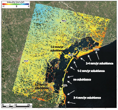
Figure 53. Venice subsidence in the period 2001.55 to 2011.00. Annual average rate of line of sight (LOS) surface displacements in mm yr−1 estimated for all of the thousands of the satellite radar permanent scatterers (Ferretti et al 2001) identified in the area. The five GPS stations are shown on white backgrounds. The rate of subsidence is shown for several locations surrounding the Venice lagoon. The velocity uncertainties range from 0.1–0.2 mm yr−1 and are based on a white noise plus flicker noise model and indicate significant subsidence (56). From Bock et al (2012a). Copyright 2012. This material is reproduced with permission of John Wiley & Sons, Inc.
Download figure:
Standard image High-resolution image8.3.2. Hydrology and drought in the western US.
Water and oil extraction have caused significant land subsidence in the western US. The most extreme example is California's Central Valley, about 250 miles in length, 40 miles in width, bounded by the Sierra Nevada to the east and the Coast Ranges to the west, with an area of 10 000 square miles, and where groundwater extraction for agriculture began in the 1920s. By the 1970s, subsidence of nearly 30 feet was recorded from spirit leveling, changing well water levels, and extensometers at several locations, with subsidence affecting about half of the valley. The trend was reversed in the 1940s and 1950s through the importation of water through the California Aqueduct. However, severe drought in the 1970s and increased water extraction caused further subsidence (Ireland et al 1984). Gravity observations from the GRACE gravity satellite from 2003 to 2010 with a resolution of about 200 km inferred that the valley lost 20 km3 of groundwater (Famiglietti et al 2011). Today, circa 2013–15, California is experiencing a severe drought. Daily vertical position time series from hundreds of stations in the state show vertical land motion due to the solid Earth's elastic response to the loading and unloading of snow and surface water (Argus et al 2014b, Amos et al 2014), aquifer charge and recharge, and drought (Borsa et al 2014b). Analysis of these data requires a careful selection of stations depending on the 'signal' of interest. In terms of the large-scale hydrological cycle, the Earth's seasonal elastic response due to loading by snow and/or rain results in upward motion, while evaporation, runoff, and desiccation result in downward motion. Therefore, stations near active aquifers need to be identified and removed from hydrological analysis so as not to obscure the regional picture, since the Earth's porous response to groundwater withdrawal (and other fluids) counteracts the elastic response. When groundwater is extracted from an aquifer such as in the Central Valley, there is downward motion due to soil compaction, while when an aquifer is recharged there is upward motion (in the winter, in California). Although analysis of the GPS network data for tectonic deformation seeks to ignore stations atop aquifers, this is often not possible because large basins in developed areas often intersect tectonically active regions (e.g. Bawden et al 2001, King et al 2007). On the other hand, anthropogenic effects (groundwater charge and recharge and oil exploration including fracking and hydrothermal mining) and natural effects (flooding) may induce seismicity or increase seismic hazards by increasing lithospheric stress (Brothers et al 2011, Amos et al 2014).
After careful removal of stations atop active aquifers, hydrological changes due to the Earth's elastic response to loading from snow and rain (the effect of the atmosphere must also be considered) can be modeled (Argus et al 2014b) using Green's functions (Farrell 1972), which are insensitive to the assumed Earth's structure (Wahr et al 2013). For a point load, the vertical displacement  in meters is given by

where  is the load mass (kg),
  is the Earth's radius (m), and the Green's function
  is a function of the angular distance between the point load and the observation site (Argus et al 2014b). GPS seasonal vertical oscillations from 1994 to 2013 were used to model seasonal surface change in equivalent water thickness as a function of location, which was compared to satellite gravity observations and hydrological models. Changes from east to west ranged from 0.6 m in the Sierra Nevada, Klamath, and the southern Cascade Mountains with a sharp decrease to about 0.1 m into the Central Valley and toward the Pacific coast. Results using a composite hydrological model from terrestrial observations of soil moisture, snow, and reservoir water showed an overall total water storage about equal to that inferred from GPS (Argus et al 2014b). A 2D elastic loading model of Earth surface flexure due to the decline in total water storage (including groundwater) was found to correlate well with average GPS vertical motions from about 120 stations transecting the Sierra Nevada, the northern section of the Central Valley (San Joaquin Valley) and the Coast Ranges. Uplift of 1–3 mm yr−1 was observed in the bordering mountains, matching current rates of water-storage loss, and most of which is caused by groundwater depletion and seasonal changes in the annual GPS displacement. This reflects the seasonal distribution in terrestrial observations of winter precipitation, snow load, and water reservoirs (Amos et al 2014). Interestingly, this study infers that the predicted upward vertical motions of the Coast Ranges reduces the effective normal stress resolved on the San Andreas fault, bringing the fault closer to failure and potentially affecting future seismicity, and that uplift in the southern Sierra Nevada is due to anthropogenic groundwater extraction, rather than solely orogenic (figure 54). Another study (Borsa et al 2014b) investigated a possible correlation in variations in the daily vertical positions of a set of hundreds of GPS stations in the western US with changes in water mass brought on by the severe California drought (circa 2013–15) compared to earlier years going back to 2003 (figure 55). After removing the stations located above active aquifers, including all the stations in the Central Valley, as well as stations with possible tectonic/volcanic induced vertical motions (e.g. the Long Valley caldera), the observed vertical displacements were inverted for elastic loads (Farrell 1972) on a 0.5° grid over the western US (figure 55). The predicted vertical displacements from the elastic loading model show a median uplift of 5 mm, with values of up to 15 mm at higher elevations (compare this to a 1–3 mm yr−1 uplift from the more focused study by Amos et al (2014) of the ranges bordering the Central Valley). This uplift corresponds to a water mass loss of up to 0.5 m, in agreement with observed decreases in the annual precipitation and streamflow in 2014. The total loss of ~240 Gt is the equivalent to a 0.1 m layer of water over the entire region; the authors of the study point out that this is about the annual mass loss from the Greenland Ice Sheet (see section 7.3).
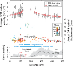
Figure 54. Swath profile of average contemporary vertical GPS velocity, annual GPS vertical displacement amplitude, and average topography from the central California Coast Range to the western Great Basin (SAF, San Andreas Fault; CT, Coalinga thrust). Uncertainties are one-sigma (66.7% confidence). The profile includes data from 121 stations and encompasses areas of the greatest historical and current change to groundwater levels. The average GPS velocity is well fitted by an elastic model simulating surface uplift resulting from the decline in total water storage (including groundwater loss) centered along and parallel to the San Joaquin Valley. Seasonal changes in the annual GPS displacement (peak-to-peak amplitude) are distributed more broadly over the San Joaquin drainage basin, reflecting distribution of winter precipitation, snow load, and reservoirs. Reproduced with permission from Amos et al (2014). Copyright 2014 Nature Publishing Group.
Download figure:
Standard image High-resolution image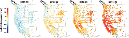
Figure 55. Drought-induced vertical land motion. Maps of vertical GPS displacements in the western US based on UNAVCO cGPS daily time series from 1 April 2011 through 1 April 2014. Uplift is indicated by the yellow-red colors and subsidence by the shades of blue. Reproduced with permission from Adrian Borsa.
Download figure:
Standard image High-resolution image
8.4. Multipath as GPS noise
The observation equations for GPS geodetic analysis (9) contain a term  referred to as antenna multipath at a particular station i. In the broader sense multipath is a result of GPS signals (dual-frequency phase and pseudorange) that are reflected or scattered by nearby objects, which interfere at the antenna with the direct signal from the satellite to the antenna. This is due to both simple reflections from the ground and other far-field surfaces, as expected from geometric optics, as well as multipath from near-field reflections, often resonant, from the antenna itself and the supporting structure. These factors need to be considered in network design. Multipath is a complex function of the geometry of the reflecting (scattering, imaging) environment, the dielectric constants of the reflectors, and the gain of the antenna (Georgiadou and Kleusberg 1988, Elósegui et al 1995, Bilich and Larson 2007, King and Williams 2009). Multipath introduces short-period (<~10 min) and diurnal signals into GPS positions, which are highly dependent on the spatial separation of the multipath source and the GPS antenna and may also have a near-annual component (Ray et al 2008). Multipath can also be exacerbated by seasonal changes at a station. For example, accumulations of snow, which retard the GPS signals and enhance signal scattering, can cause significant variations in the vertical coordinate of site position (Jaldehag et al 1996).
An approximate expression for the contribution of multipath to the observed phase in length units (Elósegui et al 1995) assumes that there exists a single horizontal, infinitely large, planar reflector distance  below the GPS antenna, and the incoming GPS signal is a plane wave with wavelength
  (L1 or L2), with incident elevation angle
  by
by
When the voltage amplitude of the reflected signal  , there is no multipath; when
  , the reflected signal has the same strength as the direct signal. At the L1 wavelength, the maximum effect is about 5 cm (Georgiadou and Kleusberg 1988). In practice, multipath is too complex to model and so its effects are effectively lumped together with random errors in the GPS model (9). This is an incorrect assumption, but no techniques have been developed to accurately quantify or measure the multipath effects of the environment around a GPS antenna for the purpose of correcting their effects in the positioning calculation.
Considering its possible magnitude, multipath is one of the limiting error sources in GPS geodesy. It is correlated with errors in the atmospheric delay, which results in a degradation in the estimate of the vertical component of position (Bock et al 2000). The vertical coordinate is already less precise than the horizontal component from geometrical considerations; GPS observations span nearly 360° in azimuth, but less than 90° in elevation. Multipath is proportional to signal wavelength and its large effect on pseudorange observations limits integer-cycle phase ambiguity resolution (section 2.4), thereby degrading the horizontal precision. The RMS of a particular combination of raw phase and pseudorange observations
is correlated with the multipath signature at a station and is often used as a metric to assess the degree of multipath (Estey and Meertens 1999). This combination removes the contributions of receiver position, atmospheric effects, satellite orbits and troposphere, ionosphere, satellite orbits and clocks, and represents the pseudorange multipath at the L1 frequency and random measurement error.
The effects of multipath can be somewhat mitigated through hardware and analysis methods. Geodetic-quality GPS antennas, often with large ground planes (figure 2), are designed to reduce the attenuation factor due to multipath, thereby improving the precision of pseudorange measurements. Spectral analysis of high-rate (1–50 Hz) GPS position time series indicates that high-frequency errors (up to several seconds) are uncorrelated from epoch to epoch, but that low frequency errors due to multipath are temporally correlated up to several min (Genrich and Bock 2006). Therefore, multipath is reduced in static applications by observing over multiple observations epochs before inversion for positions and other parameters of interest. For single-epoch positioning of static platforms, multipath effects can be significantly reduced by taking advantage of the nominal 12 h orbits of the satellites in a process called 'sidereal filtering'. The GPS satellite tracks repeat from day to day, according to the sidereal day, approximately 3 min and 56 s earlier each day because of the difference between the solar day and the sidereal day. Sidereal filtering can be performed at the observation level or the position level (e.g. Genrich and Bock 1992, Elósegui et al 1995, Bock et al 2000, Nikolaidis et al 2001, Choi et al 2004, Langbein and Bock 2004). In reality, the actual repeat time is satellite constellation dependent and may differ by several seconds so that sidereal filtering can be adjusted accordingly (Agnew and Larson 2007). Finally there are new innovations that may help reduce multipath effects for precise positioning even with smartphone-quality GPS antennas (Pesyna et al 2014), by allowing improved integer-cycle phase ambiguity resolution (section 2.4).
8.5. Multipath as signal
Antenna multipath at a GPS station has seasonal and other periodic effects due to conditions of soil, vegetation, and snow cover on the reflecting surface. Careful analysis of multipath inferred from signal to noise estimates of raw phase observations has been shown to be an indicator, through variation in frequency, phase, and amplitude, of the snow depth (Larson et al 2009, Larson and Nievinski 2013), vegetation growth (Small et al 2010) and soil moisture (Larson et al 2008, 2010) in a footprint of about 1000 m2 surrounding the GPS antenna. The frequency of multipath reflections above a horizontal plane is given by (Larson et al 2010)
that modulates the signal to noise ratio as
Here e is the satellite elevation angle above the reflector and h is the perpendicular distance of the antenna phase center from the reflector plane. The phase change  has been shown through simulation to be a function of the apparent height of the reflector relative to the antenna phase center. In the case of soil moisture, for wet soil the apparent reflector is closer to the surface than for dry soil (Larson et al 2010). For snow cover, the dominant reflector is at the air-snow interface, h is the vertical distance from the GPS antenna phase center and the snow surface, and
  is the carrier phase wavelength. Snow depth is the difference between the vertical distance of the antenna to the ground (measured during dry conditions) and the distance to the snow cover (Larson and Nievinski 2013). The observation that vegetation height and water content are inversely correlated with the magnitude of multipath, quantified by the metric
  (135) was used to distinguish between grassland, shrubland, and cropland (Small et al 2010), and, therefore, could be useful in assessing land surface conditions for agriculture as a complement to satellite remote sensing techniques.
9. Concluding perspective
9.1. Summary
After this long exposition, it is appropriate to summarize the achievements of GPS geodesy and to conclude with several open issues for ongoing and future research and development. Much more is now known about the Earth's solid surface and uppermost mantle structure, cryosphere, atmosphere, natural hazards, climate, and environment than three decades ago at the advent of the Global Positioning System. A system first conceived as a military tool has become ubiquitous, permeating civilian life, and contributing to societal well-being in ways never anticipated. The field of geodesy has evolved as its own discipline within the Earth Sciences, in large part due to the GPS. Practitioners of GPS geodesy now span the entire spectrum of scientific endeavor from hypothesis, new instrumentation, extensive field observations, data analysis, and the validation and construction of physical models. GPS geodesy is used to enhance knowledge, and support applications for the public good through early warning systems for mitigating the effects of natural hazards, for example, earthquakes, tsunamis, volcanoes, and extreme weather, and for a better understanding of anthropogenic hazards.
9.2. Infrastructure and technology
In the following we use where appropriate the more general term for navigation satellite systems, GNSS, rather than GPS, since in the near future multiple satellite constellations will provide considerable benefits to geodesy including more robustness and greater positioning accuracy, especially for real-time applications in less than optimal observing conditions (e.g. urban canyons and other locations where the sky view is partially obstructed).
The international infrastructure, conventions, and standards that have developed since the 1980s in support of GNSS applications under the auspices of the International GNSS Service (IGS) and its volunteer organizations have been the primary factor in achieving worldwide mm-level positioning capability for geodetic applications. The main IGS products include precise GNSS orbits (currently for GPS and GLONASS), satellite clock estimates, and Earth orientation parameters, which are available for real-time applications and post-processing. Another factor has been the maintenance of the International Terrestrial Reference Frame (ITRF) through the International Earth Rotation Service (IERS) based on the long history of GPS, VLBI, SLR, and DORIS observations. Until now the ITRF has been realized by a catalog of positions and velocities of the tracking stations at a particular epoch of time; the latest version is ITRF2008. An important development in the longevity and accuracy of the frame is the addition of coseismic and postseismic deformation models for stations, which have affected about one third of the stations to date. The publication of the new frame is imminent and will be defined at an epoch coinciding with the end of 2014 (ITRF2014). The formal establishment of the IGS real-time service is an important development and supports a variety of scientific and civil applications. The expansion of regional networks to thousands of stations spanning the major tectonic plate boundaries with accelerating upgrades to real-time, high-rate observations has been a boon to GNSS geodesy. Much of the data are freely available through public archives with the expectation that this will continue and be enhanced. Significant challenges for the future include continued funding for the maintenance and expansion of GNSS infrastructure globally and in regions that are not well covered. This should be facilitated through the promotion of multiple-purpose networks that disseminate data continuously, rather than disseminating them only after the next significant earthquake or geophysical event of interest. Multi-purpose real-time networks support the use of GNSS data for meteorology, space weather, short-term weather forecasting, and environmental studies, and support civilian applications such as surveying, mapping, geographic information systems, agriculture, and structural monitoring that require precise positioning in real time or in post-processing.
No measurement system stands alone and the GNSS constellations are no exception. The geodetic toolbox includes other systems mentioned in this review such as satellite radar measurements (InSAR and point scatterers), satellite altimeters and gravimeters, airborne and land-based lidar, seafloor positioning, paleogeodesy, very long baseline interferometry, and satellite laser ranging. The challenge is the optimal and holistic use of these systems through improved technology and analysis. There is also the potential to deploy the GNSS more widely on platforms that are not yet of widespread use. GNSS-equipped buoys can accurately measure tsunami waves and may only be a fraction of the cost of traditional moored deep ocean-bottom pressure sensing buoys like DART; this could enable denser observation of tsunamis than what is currently achievable, where only a handful of stations observe any given tsunami. Likewise, the integration of geodetic techniques and other types of measurement systems has not been fully exploited; we gave an example of how the GNSS, ocean-surface and ocean-bottom tsunami wave observations, seismology and seafloor positioning can be integrated for earthquake rapid response and tsunami prediction. A combination of GNSS sensors and accelerometers is already being exploited in seismogeodetic applications. In GNSS meteorology, the combination with surface pressure and temperature measurements is necessary for PW calculations; this capability will likely spread to more GNSS stations. New sensor technologies such as microelectromechanical sensors (MEMSs) are already widely used for low-cost civilian applications. Inexpensive MEMS accelerometers have been tested on shake tables and are beginning to be deployed in place of traditional observatory-grade accelerometers. Their noise levels are still orders of magnitude higher than the most sensitive accelerometers, but for a fraction of the cost they can be attractive for certain applications such as seismogeodesy, where strong ground motions are the primary observational target. Similarly, low-cost GNSS receiver boards are becoming available, which receive signals from the newer satellite constellations and modernized GPS signals providing improved accuracy and robustness for GNSS positioning. Semi-autonomous precise GNSS analysis is starting to be performed in situ rather than at a central processing facility for real-time applications that require absolute displacement such as earthquake early warning systems and the monitoring of large engineered structures such as bridges, tall buildings, and dams. This has the added benefit of reducing telemetry pressures. Broadcasting the entire GNSS observation data content is onerous and the potential to broadcast only positions from the observing site to the data center is attractive when and where available telemetry bandwidth is limited. GNSS instruments as a companion tool to inertial seismometers can substantially aid both in continuous long-term assessment of the state of health of engineered structures as well as in assessment of structural integrity immediately following large earthquakes and severe weather. In this way buildings in an earthquake stricken zone can be remotely assessed before teams of engineers are available to perform on-site inspections. In situ monitoring also reduces single point of failure, and allows the analysis of higher-rate GNSS observations (up to 50 Hz).
9.3. Science applications
9.3.1. The Earth engine.
It is interesting that space geodesy became a precise positioning tool about the same time (1970s) that the theory of plate tectonics (McKenzie and Parker 1967) was becoming widely accepted. The GPS and its predecessor space geodetic systems of very long baseline interferometry and satellite laser ranging have provided direct measurements and confirmation of plate tectonic motion, albeit only for the current instant (~40 years) of geological history. A still outstanding question is whether plate motions directly measured today with geodesy agree with the long-term (~3 Myr BP) geological estimates. It is clear that the availability of increasingly precise direct GNSS measurements of position has revealed discrepancies that have caused revisions and improvements in plate models derived from geological and magnetic anomalies. GPS geodesy has quantified the scale and magnitude of deviations from plate tectonic theory at diffuse plate boundary zones as well as intraplate deformation, although the rigidity of stable plate interiors has been found to hold at about the 1 mm/yr level, when non-tectonic effects such as glacial isostatic adjustment are accounted for. Regarding the nature of plate motion and plate boundary deformation, at what spatial scales deformation is best described by block versus continuum models is still an outstanding question (Meade 2007, Flesch and Bendick, 2007). Another question is why broad diffuse plate boundary zones are so common on land.
The GPS has played an important role in the study of crustal deformation at plate boundaries by studying the earthquake cycle and its deviations from the idealization of the Earth's crust as an elastic-brittle solid. Interseismic velocities estimated from modeling GPS displacement time series have become a critical input to fault slip rate models and have allowed the computation of global strain rates at fault system boundaries. Dense GPS measurements have revealed regions of strain segmentation, variations in interseismic coupling, in particular at subduction zones, and differentiated between locked and creeping segments of faults. GPS measurements have also been important in determining whether stress is concentrated at identifiable asperities or geometric complexities, and how this may influence earthquake rupture initiation and arrest. Furthermore, a question that will be revealed by extending the GNSS displacement record is whether these phenomena persist over multiple earthquake cycles, which will have important implications for earthquake hazard assessments. Quantifying these processes with geodetic methods will enhance our knowledge of earthquake recurrence and improve our ability to forecast the time, location, and magnitude of future events with greater confidence. Many other questions remain: How do geodetic measurements of strain accumulation compare to geologic slip rates, and how do we reconcile any differences? How are stresses transferred between faults and fault segments on different time scales and in the presence of different crustal properties (elastic versus inelastic)? What is the relationship between strain rates and the state of stress at a particular geographic location and at depth, and how can we quantify stress heterogeneity at different spatial scales?
Can we identify or place useful bounds on megathrust earthquakes? Can patterns of earthquake occurrence and strain accumulation provide useful intermediate-term forecasts of future behavior? The location of the great 2004 Mw 9.3 Sumatra–Andaman earthquake brought into question some of the basic assumptions concerning subduction zone earthquakes and underlying physical mechanisms. The unexpected occurrence of this earthquake on the northern end of the Sunda subduction megathrust, where subduction was highly oblique and rupture propagated over a distance of 1500 km contradicted the conventional wisdom that the maximum earthquake magnitude on a given thrust increases linearly with convergence rate and decreases linearly with subducting plate age. There the subducting lithosphere is old and converging at a moderate rate and there was only evidence of lower magnitude events. The occurrence of several great subduction-zone earthquakes in regions that were thought to be immune (the latest example being the 2011 Mw 9.0 Tohoku, Japan earthquake) based on the relatively short historical record indicates that any subduction zone may be a candidate for a great event whose size is limited only by the available area of the locked fault plane (McCaffrey 2008). The widespread availability of GPS velocity fields has allowed systematic studies of crustal and mantle kinematics at different styles of subduction zones and the assessment of the relative importance of the different mechanisms ongoing at subduction zones (Wallace et al 2009).
GPS coseismic displacements provide invaluable input to static and kinematic models that image the spatio-temporal details of the earthquake source and the rupture process. Their value is now well established: On their own they provide important constraints on earthquake faulting, including the location and extent of the rupture plane, unambiguous resolution of the nodal plane, and the distribution of slip. It has been further realized that the GPS offers more insight than just the static displacement field. The inclusion of high-rate GNSS time series in the inversion process has become widespread as it becomes recognized that they provide important long period information on the source process. A key benefit of GNSS coseismic measurements is to enable more reliable estimates of rapid source models. As large earthquakes over the last decade have exposed shortcomings in earthquake and tsunami early warning, the GNSS constellations are becoming recognized as a valuable and necessary addition to the repertoire of warning technologies. The combination of GNSS and traditional seismic data by seismogeodesy affords the advantages of both data types while minimizing their shortcomings.
Deviations from elastic rebound theory and the idealization of a crust as a brittle-elastic crust have been well documented by GPS displacements of postseismic deformation for all fault types. Postseismic processes, which occur without radiating elastic waves, can only be observed through geodesy. However, there are still competing models of the underlying physical processes, such as viscoelastic relaxation of the ductile lower crust and upper mantle, the poroelastic rebound of fluid-saturated crust, a combination of poroelastic relaxation above the brittle-ductile transition in the crust/upper mantle and localized shear deformation, afterslip or an increase in creep rate in the upper crust or its extension below the brittle-ductile transition, as well as constitutive rate- and state-dependent friction dynamic models extended over several earthquake cycles. Some earthquakes include more than one process. In practice, it is difficult to distinguish one postseismic process from another and to quantify the relative contributions of each. In any case, postseismic observations provide insights into crustal and mantle rheology and are useful for hazard assessment and understanding earthquake triggering. An important question is how the evolving structure, composition, and physical properties of fault zones and surrounding rock affect shear resistance to seismic and aseismic slip. Comparisons of GNSS observations and other geodetic data to physics-driven models of the crust and mantle will continue to be the most widely used method to discriminate between models.
Slow slip events indicating additional slip on subduction faults over days to months with no appreciable seismic radiation were unknown until the densification of permanent GPS networks. Slow slip events are now a source of intense study; they occur with another intriguing new discovery, tremor, and they have important implications in regards to subduction zone material properties. A big question is whether stress transfer associated with slow slip events is important in earthquake occurrence.
In spite of many of these advances, our understanding of the probability of large earthquakes on a given fault and the state absolute stress in the crust are still poorly understood. It is clear that deciphering the earthquake engine requires observations of several earthquake cycles and an improved understanding of coseismic, postseismic, and other transient deformation. Improved dynamic models of the earthquake engine over several cycles, perhaps within the rate- and state-dependent friction framework, will be the focus of future efforts; essential inputs will be longer displacement time series (the responsibility of future generations) and an increase in spatial coverage and the density of observations. Ultimately, we wish to understand the main factors that limit earthquake predictability: Are there pre-seismic signals and is prediction is even possible? Models based on laboratory-derived constitutive rate-and-state friction formulations predict that earthquakes are preceded by an accelerated creep in a nucleation zone, but this behavior has not been observed in nature.
A more promising area for the prediction and mitigation of hazards in which GNSS observations are playing a prominent role is volcano monitoring. Internal magmatic movements displace the volcano's surface and surroundings, which can be directly measured by the GNSS and other geodetic methods as possible precursors to eruption. Volcanoes erupt frequently, often accompanied by immediate significant losses of life and property, disruption to civil aviation for weeks to even months from volcanic ash, and changes in climate over years, as experienced after events such as the 1883 Krakatoa south of Sumatra, the 1991 Mount Pinatubo in the Philippines, and the 2010 Eyjafjallajökull in Iceland eruptions. Tsunamis are also caused by landslides, often the result of seismicity and pyroclastic flows from volcanic eruptions, as we described for the Stromboli volcano in Italy. We discussed that significant ocean-wide events have been postulated as a result of lateral landslides at submarine oceanic island arc volcanoes. We also discussed the use of volcanic hot spots as the basis for absolute plate motion models. The underlying physical processes that drive magmatic systems are intimately linked to plate tectonics, mantle convection, and to a holistic understanding of the Earth engine, and are still not well understood. A fuller understanding of magmatic processes and their relationship with broader crustal deformation may improve the predictive capabilities of volcano monitoring.
9.3.2. The atmosphere.
Precipitable water vapor (PW) estimates are currently available to operational weather forecasters and numerical weather prediction models with sub-hourly resolution in Europe, Japan, the US, and other locations through their respective meteorological agencies. PW has proven to be particularly useful as added empirical data to numerical models, since water vapor is such a key parameter in defining the state of the atmosphere. Assimilating precipitable water measurements from a network of GPS receivers greatly improves the forecasts of a severe storm's central pressure (Iwabuchi et al 2009). GNSS PW measurements can not only define the areal extent of moist air masses, they can also determine how moist the air is. Higher PW values are associated with monsoon-driven thunderstorms that produce flash flooding, and pose a danger to both property and human life. The ability to define the moist air mass can improve the ability to forecast thunderstorms. GNSS PW provides critical input to tracking atmospheric rivers, which are long streams of high atmospheric water vapor air that transfer moisture from tropical latitudes to mid-latitudes. When atmospheric rivers intersect a continental coast, for example in California, they often produce large amounts of relatively warm rain (Ralph et al 2006). Satellite measurements are the primary source of PW measurements over bodies of open water, but are ineffective over land and/or have latency issues related to the times of satellite overpasses. GNSS measurements complement satellite measurements of water vapor by providing similar information on land, delineating the regions of high PW, possibly associated with flood-producing rains. The availability of real-time GNSS data allows weather forecasters to track atmospheric rivers, which can produce extensive flooding damage. In addition, real-time GNSS measurements can lead to better forecasts of extreme weather through improvements to numerical forecasts. One area of research is more frequent estimates of PW at the sampling rate of the GPS receivers (1 Hz), currently produced at 5–30 min averages. Power spectrum analysis of the 1 s troposphere estimates indicates that there may be sufficient information about atmospheric turbulence to be useful for aviation. We can expect that GPS meteorology will become increasingly important to weather forecasting and that dense real-time cGPS networks (spacing of 30–40 km, the correlation length of tropospheric variations) will be upgraded with meteorological instruments, in particular with inexpensive MEMS sensors. This information will become widely accessible to the public through smart phone applications, either through the government or the private sector.
We have discussed the use of GPS data for tsunami prediction through ionospheric total electron content (TEC) disturbances generated by tsunami waves. Here we must distinguish between predictions of a tsunamigenic earthquake versus the prediction of the impact and extent of the tsunami once the earthquake has occurred. The former is still controversial, while the latter has been demonstrated. A single GNSS receiver has the unique capability of sensing the ionosphere far over the horizon. The focus of research has been to be able to generate early warning messages about 90 min prior to tsunami wave arrivals. Ionospheric TEC perturbations generated by tsunami waves are first detected at low GPS satellite elevation angle satellites. As the TEC perturbations of more GNSS satellites at higher elevation angles become available, the uncertainties associated with estimated arrival times are reduced. By 2020, there will be over 160 GNSS satellites including those of the GPS, European Galileo, Russian GLONASS, Chinese BeiDou, Japanese QZSS, Indian IRNSS, and other satellite constellations, broadcasting over 400 signals across the L-band, with double the number available today at any location, providing increased ionospheric measurement accuracy and resolution. The significant ground-network GNSS infrastructure already in place and further proliferation of real-time stations, for example in the most tsunami prone Indo-Pacific region, will provide about 90% coverage with high resolution tracking of tsunamis. Now-time products are expected to confirm the existence of actual tsunami waves in the ionosphere to reduce false alarms (assuming only actual tsunami waves will generate these signatures at that particular time and location), to estimate tsunami arrival times at coastal communities, and to generate more realistic uncertainties of the tsunami arrival time. Warning messages will be able to be issued at 15 min increments as the tsunami-generated TEC perturbations come into view of real-time stations. The GPS ionosphere-based tsunami arrival times and the associated uncertainties are expected to constrain tsunami wave height predictions for tsunami forecasters.
9.3.3. The climate and cryosphere.
GNSS geodesy is critical to the study of the Earth's cryosphere and measurements of sea level rise associated with climate change that has accelerated compared to 20th century estimates, by providing an assessment of the mass balance of the ice sheets in Greenland and Antarctica, constraints on models of glacial isostatic rebound, and the calibration of satellite-based sensors such as satellite altimeters. Estimates of the net gain or loss due to changes to ice sheets and glaciers, which have important societal impacts from climate change and the availability of adequate water resources, are not well known. The best climate models can predict changes in ice sheet accumulation through precipitation and melting but are inadequate for predicting future changes to the ice because of our limited understanding of the underlying physical processes. Therefore, continued geodetic observations from spaceborne missions coupled with in situ GNSS are critically important to an improved understanding of ice dynamics, as a basis of models to predict the response and feedback of the cryosphere to climate change (Davis et al 2012a). Continuous GNSS observations are best suited to quantify seasonal variations and ice mass accelerations and their impact on dynamic models, although operating in often inaccessible and harsh environments is a challenge.
GNSS geodesy will continue to play other critical roles in assessing climate change. The traditional use of tide gauges for measuring sea level is problematic because it measures sea level with respect to the solid Earth, which is subject to vertical land motion from anthropogenic sources such as groundwater and oil extraction, and natural processes such as large earthquakes and coastal erosion. GNSS-derived vertical displacements measured at nearby tide gauges provide a correction for possible vertical land motion. GNSS also provides input to and constraints on models of long-term glacial isostatic adjustment from the vertical trend due to the solid Earth's instantaneous elastic response to contemporary losses in ice mass, as well as to understanding the effects of seasonal variations in ice mass and atmospheric pressure. Taking these factors into account, vertical land motion and GIA have helped resolve the sea level enigma posed by W. Munk of a factor of 2 differences in sea level change between observations and modeled climatic contributions in the last half of the 20th century.
We have described how trends in the GPS surface observations of tropospheric delay supplemented by in situ pressure and temperature readings can be related to variations in atmospheric water vapor content through precipitable water vapor, and that GPS radio occultation observations of time delay of the occulted signal's phase traversing the atmosphere provide estimates of atmospheric refractivity. Long-term robust time series are now being established, from which changes in global atmospheric temperature may eventually be resolved. A long upward trend in tropospheric temperature due to increased anthropogenic CO2 emissions is predicted to produce a positive trend in atmospheric water vapor content, which is turn should enhance through a feedback mechanism the atmospheric greenhouse effect and rainfall extremes. However, the relatively short GNSS observation record (land and satellite based) has yet to show the commensurate changes. Discerning the long-term trend is complicated by the accuracy of the measurements themselves, and global and regional interannual variability such as the El Niño–Southern Oscillation (ENSO). It is clear that GNSS observations need to continue and intensify to identify long-term atmospheric variations in water vapor with their critical importance for precipitation and global water supply.
9.4. Societal implications
GPS technology has a ubiquitous presence in modern society akin to a free public utility and this will further be enhanced by new satellite constellations, the modernization of existing systems, and new signals. According to the 2014 US National Plan for Civil Earth Observations Office produced by the Science and Technology Policy Executive Office of the President, 'GPS is singularly important as the principal and irreplaceable reference for universal time and geo-reference measurements that underpin nearly all Earth observations'. In fact, this report names the GPS as the number one ranked observation system out of 145 high-impact observation systems chosen from a total of 362 systems evaluated by the US federal government. In this review paper we have covered the practice and science of GPS geodesy and discussed some of its rich applications to Earth science in areas of high societal impact as well to extreme weather forecasting and the assessment of climate change and cryosphere research as direct benefits to society.
Here we expound on other societal benefits discussed in this review including the mitigation of the effects of other natural hazards (e.g. earthquakes, tsunamis, volcanoes) and anthropogenic hazards (e.g. sea level rise due to climate change) and an improved understanding of the environment. The devastating 2011 Mw 9.0 Tohoku-oki earthquake and tsunami that claimed over 18 000 lives is a landmark event. It was the first case of a large tsunami impinging upon a heavily developed and industrialized coastline in modern times. Tsunami-induced damage to port infrastructure was heavy, major roadways and railways were severed, and energy generating power stations (in particular, at the Fukushima nuclear facility) were forced offline for extended periods of time. Defense infrastructure was compromised, telecommunications were impeded, and countless homes, offices, and other industries were destroyed. In addition to the tragic loss of life, the economic collapse of the near-source coastline, which spans nearly 400 km, was almost complete (Hayashi 2012). We discussed in detail that the earthquake was severely underestimated by the Japanese earthquake early warning system, the most advanced system in the world today, and the only one capable of generating warnings for coastal populations on-shore of the earthquake epicenter and in the gravest danger. We demonstrated that the integration of real-time GNSS displacements and accelerometer data (seismogeodesy), available in abundance in Japan, would have resulted in an accurate magnitude of the event even before the end of strong ground motion and could have been followed by improved tsunami forecasts. This could have been possible with GNSS data alone; the best possible scenario would have been the integration of existing land-based, near-coast wave observations, and seafloor pressure observations, a combination that only exists today in Japan. Whether or not these additional data would have significantly mitigated losses in 2011 will never be known for sure, but the actual response to this event provides important lessons for the future as earthquake and tsunami early warning systems become more widespread. Studies of the number of fatalities for near-source coastal communities during the 2011 Mw 9.0 Tohoku-oki earthquake and tsunami show that evacuation start time was a critical factor (Yun and Hamada 2014). The geographical extent of tsunami evacuation is predetermined by the Japanese authorities according to earthquake magnitude, which in this case was underestimated. Thus, with improved planning to consider evacuation behavior, refuge siting, the topography, and community age distribution (Yun and Hamada 2014), and with an accurate rapid estimate of earthquake magnitude the number of fatalities could be minimized during future events. In any case, a reliance on a single sensing technology is inadvisable and holistic approaches that are capable of leveraging all geophysical and other observations in a given region will be the norm for decades to come. GNSS observations are a key component in such systems.
With respect to the environment, we discussed the use of the GNSS for coastal preservation with an example of efforts to preserve the city of Venice, Italy, but there are many other coastal and island locations that are at increased risk due to rising sea levels. We also presented hydrological applications with an example of the use of GNSS displacement time series for assessing the impacts of drought in California. Finally, we discussed innovative uses of GPS 'noise' in terms of antenna multipath as an indicator of snow depth, vegetation growth, and soil moisture, with implications for agriculture, hydrology, and climate. These societal applications will be enhanced with the availability of GNSS, new innovations, improved telecommunications, and inexpensive MEMS sensors. We can expect that high-precision positioning capabilities will become ubiquitous and not only limited to geodetic applications.
Acknowledgments
We are very grateful to R King, J Haase, M Turingan and A Borsa for reading and significantly improving the manuscript. We thank M Siegfried and H Fricker for their assistance on the climate section, A Komathjy on ionosphere monitoring, A Moore and S Gutman on troposphere monitoring, and S Owen on volcano monitoring. The figures and photos were generously provided by R Allmendinger, C Amos, D Argus, G Beroza, M Bevis, A Borsa, J Church, C DeMets, D Dzurisin, M Fujita, J Haase, J Geng, J Genrich, A Ghosh, D Goldberg, R Grapenthin, W Holt, S Ide, C Kreemer, G Laske, R McCaffrey, B Meade, A Moore, A Newman, R Nikolaidis, D G Offield, L Prawirodirdjo, R Reilinger, L Rolland, L Su, C Vigny, S-I Watanabe and S Williams. We thank our colleagues at the Scripps Orbit and Permanent Array Center (SOPAC) for their contributions during the preparation of this manuscript including B Crowell, P Fang, J Saunders, M Squibb and A Sullivan, at the Caltech/Jet Propulsion Laboratory including R Clayton, E Yu, F Webb, S Kedar and Z Liu, and at NOAA including I Small, J Laber, M Jackson and S Gutman. Funding support from US government agencies including the US National Aeronautics and Space Administration (NASA) grants NNX14AQ53G, NNX12AH55G, NNX12AK24G, the US National Science Foundation (NSF) grants EAR-1252186 (EarthScope) and EAR-1252187, and the US National Oceanic and Atmospheric Association (NOAA) grant NA10OAR4320156 (CIMEC) is gratefully acknowledged. We thank the editor M Bevis for his support in making this manuscript a reality, and S Benami, V Sahakian, 'Mr' Dean McEvoy, E McEvoy, T Benami and J Benami for their inspiration. This paper is dedicated to Professor Ivan I Mueller.
Acronyms
- ALOSAdvanced Land Observing Satellite
- BARGENBasin and Range GPS Network
- C/ACoarse Acquisition code
- CDPCrustal Dynamics Project
- cGPSContinuous GPS
- CHAMPCHAllenging Minisatellite Payload for geoscientific research
- CIDCoseismic Ionospheric Disturbance
- CIPCelestial Intermediate Pole
- CMECommon Mode Error
- CMIP5Coupled Model Inter-Comparison Project phase 5
- CMTCentroid Moment Tensor
- CSDCoseismic Slip Deficit
- COSMICConstellation Observing System for Meteorology, Ionosphere, and Climate
- CpsdCycles per sidereal day
- CRFCelestial Reference Frame
- DARTDeep Assessment and Reporting of Tsunamis
- DORISDoppler Orbitography and Radiopositioning Integrated by Satellite
- ECMWFEuropean Centre for Medium-Range Weather Forecasts
- EDMElectronic Distance Measurement
- EEWEarthquake Early Warning
- ENSOEl Niño Southern Oscillation
- ENVISATEnvironmental Satellite
- EOPEarth Orientation Parameters
- ERAEarth Rotation Angle
- ESAEuropean Space Agency
- ETSEpisodic Tremor and Slip
- FCBFractional Cycle Biases
- FK-5Fifth Fundamental Catalog
- FORMOSAT-3Formosa Satellite Mission 3
- GCMGlobal Climate Model
- GCMTGlobal Centroid Moment Tensor Project
- GCRSGeocentric Celestial Reference System
- GEONETGNSS Earth Observation Network System (in Japan)
- GIAGlacial Isostatic Adjustment
- GISGeographic Information Systems
- GITEWSGerman Indonesian Tsunami Early Warning System
- GLONASSGLObal NAvigation Satellite System
- GMFGlobal Mapping Function
- GMPEGround Motion Prediction Equation
- GNSSGlobal Navigation Satellite System
- GPSGlobal Positioning System
- GPS/MetGPS/Meteorology
- GRACEGravity Recovery and Climate Experiment
- IAUInternational Astronomical Union
- ICESatIce, Cloud, and land Elevation Satellite
- ICRFInternational Celestial Reference Frame
- ICRSInternational Celestial Reference System
- IERSInternational Earth Rotation and Reference Systems Service
- IGSInternational GNSS Service
- InSARInterferometric Synthetic Aperture Radar
- IPPIonospheric Pierce Point
- IPWIntegrated Precipitable Water (or for short precipitable water, PW)
- ITRFInternational Terrestrial Reference Frame
- ITRSInternational Terrestrial Reference System
- IUGGInternational Union of Geodesy and Geophysics
- IVSInternational VLBI service for Geodesy and Astrometry
- JDJulian Date
- JMAJapanese Meteorological Agency
- JPLJet Propulsion Laboratory
- LAMBDALeast-squares Ambiguity Decorrelation Adjustment
- LiDARLight Detection and Ranging
- LODLength of Day
- MCMCMonte Carlo Markov Chain
- MJDModified Julian Date
- MLEMaximum Likelihood Estimation
- MORVELMid-Ocean Ridge VELocity
- MOSEMOdulo Sperimentale Elettromeccanico, Experimental Electromechanical Module
- NASANational Aeronautics and Space Administration
- NEICNational Earthquake Information Center
- NNR NUVEL1-ANo Net Rotation plate motion model (NUVEL-1A)
- NOAANational Oceanic and Atmospheric Administration
- PAGERPrompt Assessment of Global Earthquakes for Response
- PANGAPacific Northwest Geodetic Array
- PCAPrincipal Component Analysis
- PDFProbability Density Function
- PGDPeak Ground Displacement
- PGRPostglacial Rebound
- PPPPrecise Point Positioning
- PPP-ARPrecise Point Positioning with Ambiguity Resolution
- PTWCPacific Tsunami Warning Center
- PWPrecipitable Water
- RADARSATRadar Satellite
- RINEXReceiver Independent Exchange Format
- RMSRoot Mean Square
- SASelective Availability
- SAC-CSatélite de Aplicaciones Científicas-C
- SAFSan Andreas Fault
- SARSynthetic Aperture Radar
- SCECSouthern California Earthquake Center
- SCIGNSouthern California Integrated GPS Network
- sGPSSurvey-mode GPS
- SIOScripps Institution of Oceanography
- SLRSatellite Laser Ranging
- SSESlow Slip Event
- STA/LTAShort-Term Average / Long-Term Average
- TAIInternational Atomic Time
- TECTotal Electron Content
- TECUTEC Units
- TIDTravelling Ionospheric Disturbance
- TOPEXTopography Experiment/Poseidon
- TTTerrestrial Time
- USGSUnited States Geological Survey
- UTUniversal Time
- UT1UT corrected for polar motion
- UTCCoordinated Universal Time
- VLBIVery Long Baseline Interferometry
- VLMVertical Land Motion
- VMF1Vienna Mapping Function version 1
- WC/ATWCWest Coast / Alaska Tsunami Warning Center
- WGSWorld Geodetic System
- XYZEarth Centered Earth Fixed Coordinates
- ZHDZenith Hydrostatic Delay
- ZTDZenith Tropospheric Delay
- ZWDZenith Wet Delay
Glossary of technical terms
- Acoustic waveAn atmospheric pressure wave
- AftershockA smaller earthquake that occurs after a previous large earthquake, in the same area as the main shock
- AfterslipSlow slip on a fault in the first hours to days following an earthquake
- Ambiguity resolutionQuantification of the integer-cycle phase ambiguity
- ArcA linear volcanic chain in subduction zones
- AseismicA process that does not produce measurable elastic waves
- AsperityA portion of a fault that is locked in the interseismic period and slips suddenly during an earthquake
- AsthenosphereHighly viscous, mechanically weak and ductilely deforming region of the upper mantle of the Earth
- BackarcThe region immediately behind a subduction zone arc
- Baseline (geodesy)The distance between two observing stations
- Baseline (seismology)In the absence of motion, the deviation of a seismic instrument from a zero measurement
- CalderaA cauldron-like volcanic feature usually formed by the collapse of land following a volcanic eruption
- CalvingThe breaking off (ablation) of chunks of ice at the edge of a glacier
- Carrier waveThe waveform that is modulated onto the different GPS codes
- Celestial sphereAn imaginary sphere, useful in astronomy, which shows the celestial bodies on a finite sphere from an observer's location on the Earth (only half of the sphere is observable). The point overhead is the zenith. The horizon is the plane 90° from the zenith. The imaginary circle passing through the North and South directions on the observer's horizon and through the zenith is the celestial meridian.
- Centroid Moment TensorA point source body force equivalent model of an earthquake consisting of a 2nd order tensor and geographic location parameters
- ClippingWhen an inertial sensor reaches its maximum measurable limit
- Coarse AcquisitionCode transmitted in the GPS signal for coarse (100 m) level positioning
- CoseismicA process that occurs concurrently with or during an earthquake
- Coulomb stressA measure of the increase or decrease of the failure stress on a faulting surface
- CreepThe process whereby a fault slides continuously
- CryosphereThose portions of the Earth's surface where water is in solid form
- DewpointThe temperature at which the water vapor in a sample of air at constant barometric pressure condenses into liquid water at the same rate at which it evaporates
- DipThe steepest angle of descent of a fault relative to a horizontal plane
- Double differencingThe process of differencing the observations between two satellites and two receivers
- Draconitic yearThe time that elapses between two passages of a satellite through the ascending node of its orbit, which for GPS is 351.4 d
- Dynamic displacementRefers to sudden and rapid deformation associated with the propagation of elastic waves and with no residual permanent deformation
- Dynamic rangeThe ratio between the largest and smallest possible measurements an instrument can make
- EclipticApparent path of the Sun on the celestial sphere
- El Niño/La NiñaThe effects of a band of sea surface temperatures which are anomalously warm or cold for long periods of time that develops off the western coast of South America and cause climatic changes across the tropics and subtropics
- Electron plasmaFree electrons in the ionosphere
- EphemerisThe parameters describing the positions of satellites in orbit at a given time or times
- EpicenterThe coordinates of the surface projection of the focus or hypocenter of an earthquake
- EpochAn arbitrarily fixed date relative to which geodetic measurements are expressed
- BarystaticIn reference to sea level changes from changes of the ocean mass brought about by melting of land ice
- F layerLayer of maximum electron density in the ionosphere
- Fault finitenessTerm used to collectively describe the differences between the effects predicted by point source and finite extent models of an earthquake
- Flow-depthFlow-depth of a tsunami above the local topographic elevation
- ForearcThe region between a volcanic arc and the trench
- ForeshockAn earthquake that occurs before a larger seismic event (the mainshock) and is related to it in both time and space
- FrackingHydraulic fracturing for oil exploration
- GougeAn unconsolidated tectonite (a rock formed by tectonic forces) with a very small grain size
- Gravity waveAn atmospheric wave where the restoring force is gravity
- Ground planeA flat or nearly flat horizontal conducting surface that serves as part of an antenna, to reflect the radio waves from the other antenna elements
- Grounding lineThe interface between the floating and the grounded parts of ice
- Half-spaceEither of the two parts into which a plane divides 3D Euclidean space
- HoloceneThe geological epoch which began at the end of the Pleistocene (11 700 calendar years before the present) and continues to the present
- HypocenterThe point of initiation of earthquake rupture
- InterferogramA map of surface deformation or digital elevation, using differences in the phase of the waves returning to a satellite recorded by two or more synthetic aperture radar (SAR) scenes
- InterseismicRefers to the period in between large earthquakes where no postseismic effects from the previous rupture can be observed
- IntraplateRefers to the region within a tectonic plate
- InundationThe maximum horizontal distance of tsunami inundation
- Ionosphere delayThe delay introduced into the GPS signal by propagation through the ionosphere
- IsostasyThe state of gravitational equilibrium between the Earth's crust and mantle
- Isostatic adjustment/Post-glacial reboundThe viscoelastic response and rise of land masses that were depressed by the weight of ice sheets during the last glacial period after the ice mass is removed
- Kinematic sourceRefers to an earthquake source model that includes temporal dependence
- L1, L1C, L2, L2C, L5Shorthand for the different L-band frequencies transmitted by GPS satellites
- Last glacial maximumA period in the Earth's climate history when ice sheets were at their most recent maximum extension, between 26 500 and 19 000–20 000 years ago
- LithosphereThe outermost layer of the Earth, it comprises the crust and the portion of the upper mantle that behaves elastically on time scales of thousands of years or greater
- M-codeMilitary code for GPS satellites
- MegathrustThe contact between two converging plates at a subduction zone where large earthquakes occur
- MicroseismicitySmall background earthquakes that occur continuously in regions of active deformation
- Mid-ocean ridgeCharacteristic of extensional plate boundaries. It is an underwater mountain system that consists of various mountain ranges, typically having a valley known as a rift running along its spine
- MonsoonA seasonal reversing wind accompanied by corresponding changes in precipitation used to describe seasonal changes in atmospheric circulation and precipitation associated with the asymmetric heating of land and sea
- MonumentA geodetic marker with a measured vertical offset from the antenna reference point or a point on the antenna base
- MultipathCollectively refers to the effects of an antennas' sensitivity to, not only the direct arrival from the satellite, but from reflections of the signal by its immediate environment (vegetation, structures, etc)
- MwMoment magnitude scale for earthquakes
- Network positioningThe positioning algorithm whereby one stations position is referenced to a base station
- Neutral atmosphereThe portion of the atmosphere with no electric charge. Used to distinguish from the electron plasma in the ionosphere
- NutationShort-period changes in the direction of the Earth's axis with respect to inertial space due to tidal forces by the Sun and Moon that continuously change location relative to each other
- OccultationAn event that occurs when one object is hidden by another object that passes between it and the observer
- Outer-riseThe gentle topographic high seaward of the trench frequently observed at subduction zones
- P-codePrecision code for the GPS satellites
- P wavesPrimary seismic waves, they are compressional, low amplitude elastic waves with the fastest propagation speed
- Paroxystic explosionExplosion that is sudden and with little warning
- PlioceneGeologic timescale that extends from 5.333 million to 2.58 million years before present (BP)
- PoroelasticityThe elastic behavior of fluid-saturated porous media
- PostseismicCollectively refers to days to years following a large earthquake and the elastic and viscoelastic deformation phenomena observed during this period
- PrecessionLong-period changes in the direction of the Earth's axis with respect to inertial space due to tidal forces by the Sun and Moon that continuously change location relative to each other
- PseudorangeThe distance between a satellite and an observing station biased by possible timing errors
- PyroclasticA material composed solely or primarily of volcanic rocks. Where the volcanic material has been transported and reworked through mechanical action
- QuaternaryThe current and most recent of the three periods of the Cenozoic Era in the geologic time scale. It follows the Neogene Period and spans from 2.588 ± 0.005 million years ago to the present.
- RadiosondesA battery-powered telemetry instrument package carried into the atmosphere, usually by a weather balloon
- RakeThe angle between the direction of slip of a fault and the strike line of the fault plane
- Rate and state frictionPhenomenological constitutive laws to describe the frictional behavior of materials
- RegularizationNumerical technique for the solution of ill-conditioned inverse problems
- RiftA linear zone where the Earth's crust and lithosphere are being pulled apart characterized by a central depression
- Rise-timeThe time taken for a fault, or a portion thereof, to slip
- Run-upThe maximum on-land amplitude of a tsunami referenced to a vertical datum such as mean sea level
- S wavesSeismic secondary waves. Elastic shear waves with larger amplitude than P-waves but slower propagation speeds
- SaturationA condition where an earthquake magnitude scale cannot differentiate earthquakes of increasing magnitude
- Scaling relationshipEmpirical relation relating ground motion, source dimensions or other similar parameters to earthquake magnitude
- SeasonalRefers to signals with semiannual or quarterly periods
- Seismic momentA measure of an earthquake's size, it is the product of average slip on the fault, fault area, and rigidity of the sheared rock
- Seismogenic zoneThe zone within the crust or lithosphere over which most earthquakes are initiated
- Selective availabilityThe ability to add intentional, time varying errors of up to 100 m to the publicly available GPS navigation signals
- Sidereal filterA technique to reduce multipath noise by taking advantage of the nominal 12 h orbits of GPS satellites
- SillA tabular sheet of igneous rock intruded between and parallel with the existing strata
- SlabThe downgoing portion of the lithosphere in a subduction zone
- SlipThe relative displacement between two sides of a geologic fault
- Slow-slip eventSlip on a fault at very low speeds that produces no measurable elastic waves
- Source time functionThe function that describes the time-dependent release of seismic moment at a fault
- Spirit levelingA technique to find the elevation of a given point with respect to the given or assumed datum using a spirit level
- Static displacementRefers to the permanent coseismic deformation after an earthquake
- Static sourceAn earthquake source model with no information on the temporal evolution of the event
- StericIn reference to sea level, changes produced through thermal expansion
- Stick-slipThe spontaneous jerking motion that can occur while two objects are sliding over each other
- StratovolcanoA conical volcano built up by many layers (strata) of hardened lava, tephra, pumice, and volcanic ash
- Stress-dropThe difference between the stress on a fault before and after an earthquake
- StrikeThe angle between north and a horizontal line on a fault
- Strong motionRefers to high intensity shaking in seismology, typically whenever an earthquake is widely felt
- SubductionThe process that takes place at convergent boundaries by which one tectonic plate moves under another tectonic plate and sinks into the mantle
- Surface waveAn elastic wave that propagates at the interface between the crust and the atmosphere
- SwarmA sequence of many earthquakes striking in a relatively short period of time within a confined geographic location
- SynopticIn climatology, refers to length scales of thousands of km and time scales of the order of weeks
- TillUnsorted fine grained glacial sediment
- TransformA lateral fault or plate boundary where two blocks slide laterally to each other
- TransientA short-lived episode of anomalous station motion
- TremorLow amplitude, long lived seismic shaking related to slow-slip events
- TrenchLong and narrow topographic depressions of the seafloor associated with subduction zones
- TropopauseThe boundary in the Earth's atmosphere between the troposphere and the stratosphere
- Tropospheric delayThe delay introduced into the GPS signal due to propagation through the troposphere
- Universal timeA time standard based on the Earth's rotation (no longer used in civilian timekeeping), UT1 is UT corrected for polar motion
- Universal coordinated time (UTC)Atomic time that serves as the basis of civilian timekeeping
- Velocity-strengtheningRefers to a type of material whose frictional properties produce stick-slip behavior at a fault zone
- Velocity-weakeningRefers to a type of material whose frictional properties produce stable sliding or creep at a fault zone
- W-PhaseA long period seismic phase arriving between the P and S waves used for CMT calculation in seismology
- Weak-motionRefers to low amplitude seismic signals imperceptible to humans