


ABSTRACT
We use Kepler short-cadence light curves to constrain the oblateness of planet candidates in the Kepler sample. The transits of rapidly rotating planets that are deformed in shape will lead to distortions in the ingress and egress of their light curves. We report the first tentative detection of an oblate planet outside the solar system, measuring an oblateness of  for the 18 MJ mass brown dwarf Kepler 39b (KOI 423.01). We also provide constraints on the oblateness of the planets (candidates) HAT-P-7b, KOI 686.01, and KOI 197.01 to be <0.067, <0.251, and <0.186, respectively. Using the Q' values from Jupiter and Saturn, we expect tidal synchronization for the spins of HAT-P-7b, KOI 686.01, and KOI 197.01, and for their rotational oblateness signatures to be undetectable in the current data. The potentially large oblateness of KOI 423.01 (Kepler 39b) suggests that the Q' value of the brown dwarf needs to be two orders of magnitude larger than that of the solar system gas giants to avoid being tidally spun down.
Export citation and abstract BibTeX RIS
1. INTRODUCTION
The solar system planets are oblate in shape due to their rapid rotations. The equatorial radius is larger than the polar radius by 7% for Jupiter, and by 10% for Saturn. The bulk rotational angular momentum of a planet is retained from gas accretion in the formation process (e.g., Lissauer 1995). For a planet in hydrostatic equilibrium, the level of deformation is related to the rotation rate and moment of inertia of the planet, which in turn are influenced by its density profile (Hubbard & Marley 1989; Murray & Dermott 1999; Carter & Winn 2010a). Measuring the oblateness of exoplanets will enable us to better understand their interior structure, as well as their formation and evolutionary history.
Previous works (Hui & Seager 2002; Seager & Hui 2002; Barnes & Fortney 2003; Carter & Winn 2010a, 2010b) explored the predicted transit light curves of oblate planets. The transit light curve of an oblate planet is asymmetric about the ingress and egress regions, and will exhibit small differences over ingress and egress to the transit of a spherical planet. However, it is difficult to photometrically measure the oblateness of an extrasolar planet due to its small amplitude signature. For an optimal case—a transiting Jupiter with planet-to-star radius ratio of 0.15 and a Saturn-like oblateness of 0.1—the maximum deviation between an oblate and a spherical planet transit is 400 parts per million (ppm) over the ingress and egress light-curve regions (Carter & Winn 2010a).
The only implementation of oblate transit models to date was carried out by Carter & Winn (2010a), with seven transits of the hot Jupiter HD 189733b observed by the Spitzer Space Telescope. They were able to rule out a Saturn-like oblateness for the planet. HD 189733b and other hot-Jupiters, with orbital semi-major axes <0.2 AU, are expected to have spun down due to tidal dissipation and to be tidally locked. The photometric signatures due to oblateness from these slowly rotating gas giants are too small to be measurable by any current facility.
The unprecedented photometric precision of the Kepler mission has enabled the detection of many subtle photometric effects, such as phase curves of reflected light from planets (Borucki et al. 2009), Doppler beaming (Mazeh et al. 2012), and gravity-induced asymmetry due to system spin–orbit misalignments (Barnes et al. 2011; Zhou & Huang 2013). The four year baseline of Kepler also means that observations of planetary transits are no longer restricted to short-period systems. The possibility of observing the transits of gas giants that are not tidally affected and thus still retain their primordial spin rate motivates a new search for oblateness signals in-transit light curves. This work is the first survey to use Kepler short-cadence photometry to measure the oblateness of transiting planets.
The structure of this paper is as follows. Section 2 describes the light-curve modeling of a transiting oblate planet, and discusses the detectability of such a signal. Section 3 describes the target selection and Kepler light-curve reduction procedures. We apply the oblate planet transit model to Kepler light curves in Section 4, first as a signal injection and recovery exercise to demonstrate the detectability of the signal, then to model four selected Kepler planet candidates. In Section 5, we discuss the implications of our results.
2. LIGHT-CURVE MODEL
2.1. The Transit of an Oblate Planet
The shape of an oblate planet can be quantified by the flattening, or oblateness, parameter f,

where Req and Rpol are the equatorial and polar radii, respectively (Murray & Dermott 1999). We also define the effective mean radius to be

which is the radius of a spherical planet of the same cross-sectional area. The planet's spin obliquity, θ, is defined as the angle between the polar axis of the planet and the orbital angular momentum vector (Carter & Winn 2010a).
The flattening f can be related to the rotation period Prot of a planet with mass Mp by

where J2 is the quadrupole moment (Carter & Winn 2010a).
However, what we can measure from transit is not the true flattening and obliquity, but their projected components on the plane of the sky, f⊥ and θ⊥, meaning that the constrained oblateness from transit is only a lower limit on the true oblateness. The relations between f, θ and f⊥, θ⊥ can be found in Carter & Winn (2010a). The definition for the sign of θ⊥ is shown in the upper panel of Figure 2.
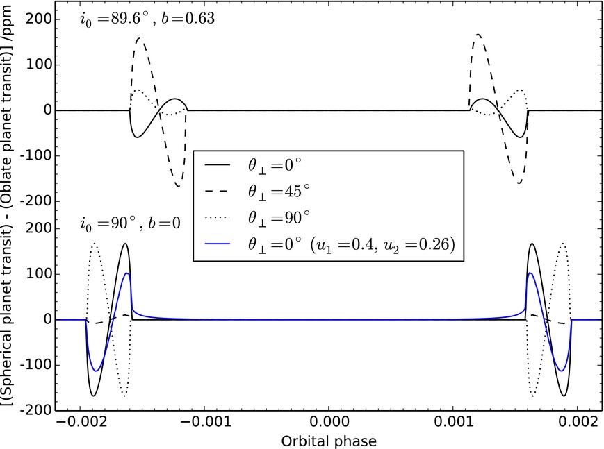
The transit light curve of an oblate planet is described by the intersection between an ellipse and a circle. For the ingress and egress regions of the light curve, where the deviation from a spherical planet model light curve is greatest, we compute the intersection region using the quasi-Monte Carlo integration algorithm introduced by Carter & Winn (2010a).6 For the in-transit regions, where the planet is fully within the stellar disk, we replace the oblate planet signal with a spherical planet with the same cross-sectional area. Since Rp ≪ R⋆, we assume the spatial limb darkening variation within the area covered by the planet ellipse is negligible. In fact, the in-transit signal induced by limb darkening is <10 ppm even for planets with substantially large Rp/R⋆ (Carter & Winn 2010a), which is insignificant for the purpose of model fitting compared with the noise level (∼500 ppm) of Kepler short-cadence light curves. By replacing the oblate planet with a spherical planet for the in-transit region, we are able to speed up the original algorithm introduced by Carter & Winn (2010a) by a factor of 10. We demonstrate in Figure 1 the theoretical oblateness-induced signal for a Jupiter-size planet in a 100 day orbit around a Sun-like star with uniform surface brightness (i.e., no limb darkening effect). We assume the planet has a Saturn-like oblateness (f⊥ = 0.1, note that fsaturn = 0.098). Signals from different projected planet spin obliquities θ⊥ (0°, 45°, 90°) are plotted for comparison. We also add an example signal from the oblate planet transiting a limb-darkened stellar surface in Figure 1, with the in-transit signal considered, to show the influence of the limb darkening effect.

Figure 1. Example signals induced by an oblate planet with respect to a spherical planet of the same cross-sectional area, for θ⊥ = 0, 45, 90°, at b = 0.63 (top) and b = 0 (bottom). These signals are for a Jupiter-size (Rp/R⋆ = 0.1) planet with a Saturn-like oblateness (f⊥ = 0.1). The black curves are computed for stars with uniform surface brightness, and the blue solid curve is for a limb-darkened Sun-like star.
Download figure:
Standard image High-resolution imageAs Figure 1 shows, the oblateness-induced signal is at least an order of magnitude greater over ingress and egress than the in-transit part. The theoretical maximum amplitude of the signal at the ingress/egress part can be estimated by

which can be achieved when the impact parameter satisfies the following condition:

The derivation for this expression of the maximum achieved signal is shown in detail in Appendix A. Although Equation (3) is useful in estimating the amplitude of an oblateness-induced signal, one should keep in mind that the recovered signal from light-curve modeling may have a smaller amplitude due to slight changes in those from other fitting parameters, especially when the oblateness-induced signal is mirror symmetric (Barnes & Fortney 2003). Space-based observations, such as Kepler, can achieve photometric precision comparable to this signal amplitude (Jenkins et al. 2010; Gilliland et al. 2010; Murphy 2012), making possible the detection of planetary oblateness when multiple transits are observed.
It is also useful to have a comprehensive understanding of the amplitude of the oblateness signal for arbitrary projected obliquity angles, θ⊥, and impact parameters, b0. To achieve this, we simulated theoretical light curves on a grid of θ⊥ and b0 with fixed f⊥ and Rp/R⋆. For most of the ranges of θ⊥ and b0 we consider, assuming a moderate projected oblateness f⊥ (≲ 0.2), that Equation (3) can be written as

In Figure 2 we show an example of Signalmax(Rp/R⋆, f⊥, θ⊥, b0) with Rp/R⋆ = 0.1 and f⊥ = 0.1. This figure tells us that the amplitude of an oblateness signal reaches maximum at θ⊥ ∼ 0° for a system that is very close to edge-on, and at larger (absolute) projected obliquities as the system becomes more inclined. Particularly, for b0 ≈ ±0.7, the signal will have maximum amplitude at θ⊥ ≈ ±45°, where the shape of the signal becomes the most asymmetric (see Figure 1). This is why the detectability of oblateness is maximized at b ≈ 0.7, as determined numerically by Barnes & Fortney (2003). The values of θ⊥ where the maximum amplitude of signal is achieved are also those where the oblateness can be most tightly constrained. We will further demonstrate this point in the modeling of simulated signal and real data.

Figure 2. Upper panel: three schematic system configurations to demonstrate the definition of θ⊥; the shape and relative size of the planet are not scaled for a realistic planet. Lower panel: the amplitude of oblateness signal as a function of the impact parameter b0 and the projected obliquity θ⊥; a Jupiter-size (Rp/R⋆ = 0.1) planet with a Saturn-like oblateness (f⊥ = 0.1) is assumed.
Download figure:
Standard image High-resolution imageIf limb darkening is considered, the maximum amplitude decreases by a factor of 6(1 − u1 − u2)/(6 − 2u1 − u2), where u1 and u2 are the quadratic limb darkening coefficients (Claret 2000).
2.2. Detectability in Kepler Data
As discussed in Section 2.1, for a Jupiter-size planet (Rp/R⋆ = 0.1) with Saturn-like oblateness (f = 0.1), the maximum signal amplitude due to oblateness is ∼160 ppm.
The signal-to-noise ratio (S/N) for a single transit in the white noise limit can be estimated by

in which, ootv is the out-of-transit variation amplitude (per point) and Np denotes the number of observations during the ingress/egress time. The duration of the ingress/egress time τ can be estimated by

For a 12 magnitude star, the Kepler long-cadence data can typically achieve a photometric precision of 100 ppm. Assuming white noise, the equivalent out-of-transit scattering (ootv) of the corresponding short-cadence data is ∼550 ppm, which corresponds to S/N ∼3. We note that this S/N estimation is almost exact for short-cadence data, with the oblateness-induced signal sufficiently mapped out by the 1 minute cadence. Transits having only long-cadence data will typically have a much shallower signal than the theoretical value, given that the signal duration is roughly comparable to the long integration time (30 minutes). For example, for a Jupiter-size planet in a 15 day orbit, the ingress/egress duration is ∼30 minutes, and thus the oblateness signal is strongly suppressed in the long-cadence data. For this reason, we do not consider the long-cadence data in the present work.
With Kepler light curves from Q1–Q16 (∼1400 days), we expect a planet with a 100 day orbital period and a Saturn-like oblateness to be detected with a S/N ∼11 in the white noise limit. In the red noise limit, S/N would scale with the number of transits instead of the number of data points observed, which would reduce the expected S/N severely.
3. TARGET SELECTION AND LIGHT-CURVE TREND REMOVAL
We select Kepler planet candidates from Q1 to Q16 (Batalha et al. 2013; Burke et al. 2014) with the following criteria:
- 1.candidates with radius smaller than 2.0 RJ, to avoid eclipsing binaries;
- 2.orbital periods longer than 15 days, such that the spin–orbit synchronization timescale of the planet is greater than 250 Myr, assuming a Jupiter-mass planet around a solar-mass star (Carter & Winn 2010b);
- 3.the transit is not grazing (b < 0.8), such that the transit system parameters are well constrained;
- 4.expected S/N for a planet with a Saturn-like oblateness is higher than 0.5 for a single transit.
We use Equation (6) to compute the S/N per transit for each candidate. The ootv value is the point-to-point scatter of the light curve, measured over the regions on either side of the transit event, with a width of half transit duration. The actual expected S/N will be multiplied by the square root of the available number of transits from Kepler data. In addition, we did not select those systems with strong transit timing variations because it leads to more complexity in the modeling. Eleven candidates pass the above threshold, among which, only three have short-cadence data. We select these three targets, KOI 686.01, KOI 197.01, and KOI 423.01 (Kepler 39b), as examples for the modeling. We note that these three targets together are not a statistically meaningful sample since our selection criteria are somewhat arbitrary. We also modeled HAT-P-7b (KOI 2.01), despite the fact that it is a hot Jupiter and outside our period selection range, because it will provide a direct comparison to the modeling of HD 189733b in Carter & Winn (2010a).
To characterize our detection sensitivity to the oblate planet signals, we perform a signal injection and recovery exercise using the light curves of KOI 368. The 11.3 mag star is photometrically quiet, with near-minimum ootv of a bright star in the Kepler band. The KOI 368 system, with 110 day period, resembles an ideal system, with near-optimal oblateness S/N detectability. We chose not to fit for oblateness in the actual transits of KOI 368.01, because KOI 368.01 is an M dwarf, not a planet, and the modeling would require a simultaneous fit of the stellar gravity darkening effect (Zhou & Huang 2013) and the planet oblateness effect, which is outside the scope of this study.
We detrended all available public Kepler short-cadence light curves of the above targets for our analysis. To remove the stellar variability, we use the raw flux (Simple Aperture Photometry,  ) obtained from the MAST archive,7 with the out-of-transit variations corrected by the following steps from Huang et al. (2013):
- 1.removal of bad data points;
- 2.correction of systematics due to various phenomena of the spacecraft, such as safe modes and tweaks; and
- 3.we use either a set of cosine functions with minimum period of three times the transit width (Kipping et al. 2013) to fit over the out-of-transit regions and correct the trend in the light curves if there are high amplitude, short term (1 day to 20 days) variations present in the light curves. Otherwise, we use a seventh-order polynomial as our fitting function for the out-of-transit variations.
4. LIGHT-CURVE FITTING AND RESULTS
In this section, we first perform a signal injection and recovery exercise with simulated transits of KOI 368.01 to demonstrate the modeling and fitting process. We then present the modeling of the four selected systems: HAT-P-7b (KOI 2.01), KOI 686.01, KOI 197.01, and KOI 423.01 (Kepler 39b). We first fit a standard Mandel & Agol (2002) transit model to the light curves, with the free parameters being the orbital period P, transit epoch T0, planet-to-star radius ratio Rp/R⋆, normalized orbital semi-major axis (Rp + R⋆)/a, line-of-sight inclination i, and quadratic limb darkening parameters q1 and q2 parameterized according to Kipping (2013):

For the initial positions of the minimization we use system parameters from the cumulative Kepler planetary candidate table of the NASA Exoplanet Archive8 and limb darkening coefficients from Sing (2010). We then introduce the oblateness parameters f⊥ and θ⊥ and rerun the minimization using the oblateness model with the best-fit values from the standard model fit as starting points. To avoid artifacts from boundary conditions, we allow f⊥ to vary from −0.6 to 0.6, taking the absolute value and then folding the negative and positive f⊥ steps together in the final analysis. Similarly, we also allow periodic boundary conditions for θ⊥ between −90° and 90°.
For each minimization, we perform a Markov Chain Monte Carlo (MCMC) analysis to find the best-fit parameters and the associated uncertainties using the emcee ensemble sampler (Foreman-Mackey et al. 2013). In each fitting routine, we employ 150 walkers each with 4000 iterations. We chose the number of walkers to match the suggested acceptance rate by emcee. After the MCMC routine finishes, we flatten the whole chain and discard the initial steps (⩽25%) where the sampling has not burnt in. We confirmed the convergence of the chain by splitting the whole chain, after the burn-in steps were discarded, into two parts and comparing the posteriors from them.
We give the comparison between the Kepler parameters and our best-fit parameters for each planet. As in Carter & Winn (2010a), for most parameters, we report the median of the posterior probability distribution, along with error bars defined by the 16% and 84% levels of the cumulative distribution. For the projected oblateness f⊥, we report the 68% confidence upper limit if the peak of f⊥ has no obvious deviation from zero. Otherwise we report the median value, together with the 16% and 84% levels of the cumulative distribution as the error bars. We do not report constraints on the projected obliquity because it is weakly constrained, as Carter & Winn (2010a) has shown.
For each system, we also inject null signal transit light curves, resembling that of a spherical planet with the same system parameters as the target system, into different out-of-transit sections of the SAP light curve. The injected transits are shifted in time to the same epochs as the true transits. The simulated null-case transits are then processed in the same way as the observed transits.
4.1. Injection and Recovery Simulations with KOI 368.01
To demonstrate the detectability of the oblateness signal, we perform a signal injection and recovery exercise using out-of-transit light-curve segments from the KOI 368 system. KOI 368 is a photometrically quiet A dwarf hosting a transiting M dwarf with P = 110.32 days, Rp/R* = 0.084, i = 89.36 (b = 0.64), and limb darkening coefficients u1 = 0.23, u2 = 0.29 (Zhou & Huang 2013). The KOI 368 light curves and system properties resemble the transits of an optimal case, long-period planet candidate. We inject 12 transits of an oblate planet with the same system parameters as KOI 368.01, and f⊥ = 0.1 and θ⊥ = 45°, onto random segments of the SAP short-cadence light curves of KOI 368. The injected transit yields an oblateness signal with amplitude 80 ppm. In contrast, the out-of-transit variation amplitude of the light curves is 300 ppm.
The simulated light curve is then processed by our standard detrending pipeline (see Section 3) and fitted with the MCMC method. For comparison, we also report the results with standard Mandel–Agol transits injected in the same segments and detrended in the same way. In each case, the simulated data is fit first by a standard transit model and then an oblate planet model. To demonstrate the least and most optimal cases, we present the injection and recovery for the case of a single transit and the case of all 12 full transits for the KOI 368 system. The light curves and the residuals to the standard and oblate planet models (for the 12 transits case) are shown in Figure 3.

Figure 3. Simulated transit of an oblate planet using the same system parameters as that of KOI 368.01, with oblateness of f⊥ = 0.1 and obliquity θ⊥ = 45°, into the out-of-transit light curve of KOI 368 (top). The fit residuals with 12 transits to the best-fit oblate planet model (middle panel) and the best-fit standard transit model (bottom panel) are plotted. We binned the data in the phase space with a 150 points moving window and show the median and scattering in the black dots.
Download figure:
Standard image High-resolution imageThe signal is detected at a significant confidence level in our oblate planet model fitting. The original injected oblateness f⊥ is recovered in the single transit case. The left panels in Figure 4 show the posterior distributions from the fitting of a single injected short-cadence transit that contains the oblateness signal. Although the projected obliquity suffers the degeneracy between f⊥ and θ⊥, and is therefore not well recovered, the asymmetry between θ⊥ > 0 and θ⊥ < 0 implies that the true value should be positive.

Figure 4. Panel (a): two-dimensional posterior distributions for the projected oblateness f⊥ = 0.1 and obliquity θ⊥ = 45° of a single simulated KOI 368.01 oblate planet transit. Panel (b): posterior distributions for the simulated KOI 368.01 standard Mandel–Agol transit (null case). Panels (c) and (d): marginalized distributions of f⊥ and θ⊥ for simulated cases with (red) and without (black) the oblateness signal.
Download figure:
Standard image High-resolution imageFor comparison, the posteriors of the null case are shown in the right panels of Figure 4. The null case is also an example that can be used to demonstrate the ability of constraining the oblateness with Kepler data. From the fitting of a single injected transit, an oblateness as large as that of Saturn can be ruled out if the planet has moderate obliquity. However, the constraint we can place at θ⊥ = 0°, ±90° is very weak, because for this case b = 0.64 and the oblateness signal can still be very small even for large oblateness, as shown in Figure 2.
The correlations between oblateness parameters f⊥, θ⊥, and other transit parameters derived from the MCMC fitting of a single injected oblate planet transit are shown in Figure 5. f⊥ appears to be correlated with (Rp + R⋆)/a, Rp/R⋆, and i0, and shows long tails toward large oblateness in each plot, because θ⊥ is only weakly constrained. These correlations suggest that one might get systematic biases on the planetary parameters if an oblate planet is fit with a spherical model. It is worth noting that the f⊥ is hardly correlated with the limb darkening coefficients q1 and q2.

Figure 5. Correlations between f⊥, θ⊥, and other transit parameters, as derived from the single simulated KOI 368.01 oblate planet transit.
Download figure:
Standard image High-resolution imageWhen the number of transits is increased to 12, the injected signal is recovered with a significantly higher confidence level, as shown in Figure 6. We can see the oblateness signal visually in the residual (from all 12 transits) of the fitting using only the standard Mandel–Agol model in Figure 3. For the null case, we can successfully rule out an oblateness as small as that of Uranus for most θ⊥. The injected parameters, and the recovered parameters from standard model and oblateness model are shown in Table 1.

Figure 6. Posterior distributions as recovered from 12 injected KOI 368 oblate planet transits. Figure captions as per Figure 4.
Download figure:
Standard image High-resolution imageTable 1. Signal Injection and Recovery Parameters for KOI 368 (12 Transits)
| Parameters | Injected (Oblate Model) | Standard Model | Oblate Model | Injected (Standard Model) | Oblate Model |
|---|---|---|---|---|---|
| q1 | 0.27 | 0.26 ± 1 | 0.25 ± 1 | 0.27 | 0.25 ± 1 |
| q2 | 0.22 | 0.23 ± 5 | 0.24 ± 4 | 0.22 | 0.25 ± 5 |
| Porb (days) | 110.321645 | 110.32167 ± 2 | 110.32166 ± 2 | 110.321645 | 110.32166 ± 2 |
| t0 (BJDUTC-2454000) | 1030.36409 | 1030.3639 ± 1 | 1030.3639 ± 1 | 1030.36409 | 1030.3639 ± 1 |
| (Rp + R⋆)/a | 0.02097 | 0.02103 ± 4 | 0.02101 ± 5 | 0.02097 | 0.02103 ± 5 |
| Rp/R⋆ | 0.08408 | 0.0842 ± 1 | 0.0842 ± 1 | 0.08408 | 0.0842 ± 2 |
| i0 (deg) | 89.204 | 89.199 ± 3 | 89.200 ± 4 | 89.204 | 89.199 ± 4 |
| f⊥ | 0.1 | ⋅⋅⋅ | 0.11 ± 3 | 0 | <0.03 |
Download table as: ASCIITypeset image
4.2. HAT-P-7b (KOI 2.01)
HAT-P-7b orbits around a slightly evolved F star in a 2.2 day orbit (Pál et al. 2008). A planet in such a close-in orbit is believed to be tidally locked, and therefore HAT-P-7b should not exhibit rotation-induced oblateness. We include this planet in our sample for a number of reasons. First, this planet has been observed with short-cadence mode for the entire Kepler operation time. There are in total 591 full transits of HAT-P-7b within the Q1 to Q16 short-cadence data. The 1 minute cadence out-of-transit variation is 234 ppm. This allows us to directly compare our modeling result with that of HD 189733b, the only other hot-Jupiter with its oblateness constrained by observations (Carter & Winn 2010a). Furthermore, there are various other photometric effects present in the HAT-P-7 light curves, such as the intrinsic stellar variability, planetary phase variations, stellar ellipsoidal variations (Borucki et al. 2009), and possible planet-induced gravity darkening effects (Morris et al. 2013). An analysis of HAT-P-7b can also help us understand how these effects influence our oblateness model fitting procedure. We list the physical parameters of the host star in Table 2.
Table 2. Physical Parameters about the Host Star HAT-P-7 (KOI 2.01, KIC 10666592)
| Parameters | Values |
|---|---|
| Teff (K) | 6350 ± 80a |
| log g (dex) |  a a |
| [Fe/H] (dex) | +0.26 ± 0.08a |
| M⋆ (M☉) |  a a |
| R⋆ (R☉) |  a a |
| vsin i⋆ (km s−1) | 3.8 ± 0.5a |
| J-band mag | 9.555 |
| H-band mag | 9.344 |
| K-band mag | 9.334 |
Note. aAdopted from Pál et al. (2008).
Download table as: ASCIITypeset image
Fitting all 591 short-cadence transits is extremely computationally expensive. It may also produce questionable results given the systematic transit depth variations between different quarters (Van Eylen et al. 2013). We therefore fit the light curve of HAT-P-7b in three groups of 100 consecutive orbits each. The MCMC chains from the three groups are combined afterward to arrive at the global best-fit parameters. Examining the individual group results will also allow us to better judge the effect of stellar variability and red noise on the consistency of our results. Our best-fit parameters for both standard and oblateness fittings, together with the initial parameters from Kepler, are listed in Table 3. We show in Figure 7 the upper limits of f⊥ for different θ⊥. The overall 68% upper limit on the oblateness is 0.067. The oblateness is only weakly constrained around θ⊥ = 0° and ±90°, which results in the small bump around 0.1 in the posterior distribution of f⊥. However, if the planet is moderately tilted, an oblateness as large as that of Neptune (0.017) can be ruled out with 95% confidence. This constraint is comparable to that placed on HD189733b by Carter & Winn (2010a), who ruled out a Uranus-like oblateness (0.023; 95% confidence) for most of the projected obliquity angles and placed an overall 95% upper limit of 0.058 on the planet.

Figure 7. Posterior distributions for the projected oblateness f⊥ and obliquity θ⊥ for HAT-P-7b. (a) The two-dimensional posterior of f⊥ and θ⊥ are plotted. The true oblateness of Saturn, Jupiter, and Neptune are marked for reference. The marginalized one-dimensional posteriors for f⊥ and θ⊥ are also plotted in panels (b) and (c), respectively.
Download figure:
Standard image High-resolution imageTable 3. Fitting Parameters of HAT-P-7b
| Parameters | Kepler | Standard Model | Oblate Model |
|---|---|---|---|
| q1a | 0.28 ± 2b | 0.28 ± 1 | 0.28 ± 1 |
| q2a | 0.33 ± 1b | 0.33 ± 1 | 0.33 ± 1 |
| Porb (days) | 2.2047354 ± 1 | 2.2047350 ± 3 | 2.2047349 ± 3 |
| t0 (BJDUTC-2454000) | 954.35780 ± 2 | 954.35860 ± 2 |  |
| (Rp + R⋆)/a | ⋅⋅⋅ | 0.2595 ± 4 |  |
| a/R⋆ | 4.7 | ⋅⋅⋅ | ⋅⋅⋅ |
| Rp/R⋆ | 0.07545 ± 2 | 0.07748 ± 4 |  |
| i0 (deg) | 88.2 | 83.13 ± 5 |  |
| f⊥ | ⋅⋅⋅ | ⋅⋅⋅ | <0.067 |
Notes. aq1 and q2 are calculated using Equations (8) for the "Kepler model." bAdopted from Van Eylen et al. (2013).
Download table as: ASCIITypeset image
4.3. KOI 686.01
KOI 686.01 (KIC 7906882) is a planetary candidate with an orbital period of 52.51 days and a planet-to-star radius ratio Rp/R⋆ = 0.12, orbiting around a G-type star with a Kepler-band magnitude of 13.58. The physical parameters of the host star are listed in Table 4.
Table 4. Physical Parameters about the Host Star KOI 686 (KIC 7906882)
| Parameters | Values |
|---|---|
| Teff (K) | 5559 ± 71 |
| log g (dex) | 4.47 ± 0.3 |
| [Fe/H] (dex) | −0.18 |
| M⋆ (M☉) | 0.869 ± 0.051 |
| R⋆ (R☉) | 0.9 ± 0.35 |
| J-band mag | 12.270 |
| H-band mag | 11.931 |
| K-band mag | 11.847 |
Download table as: ASCIITypeset image
We assign epoch zero to the first transit observed by Kepler. KOI 686.01 has only one short-cadence full transit at epoch +12. The out-of-transit variation amplitude of this transit is 851 ppm. After reducing the data according to Section 3, we fit this short-cadence transit to a standard transit model, using the parameters given by Kepler as initials. With the best-fit parameters given by the standard transit model, we then set f⊥ and θ⊥ free to allow the oblateness fitting. Our best-fit parameters for both standard and oblateness fittings, together with the initial parameters from Kepler, are listed in Table 5.
Table 5. Fitting Parameters of KOI 686
| Parameters | Kepler | Standard Model | Oblate Model |
|---|---|---|---|
| q1 | 0.46 ± 7 | 0.29 ± 15 |  |
| q2 | 0.34 ± 2 | 0.39 ± 29 |  |
| t0 (BJDUTC-2454000) | 1004.6737 ± 1 | 1004.6743 ± 2 | 1004.6743 ± 2 |
| (Rp + R⋆)/a | ⋅⋅⋅ | 0.0108 ± 2 |  |
| a/R⋆ | 109.3 ± 4.2 | ⋅⋅⋅ | ⋅⋅⋅ |
| Rp/R⋆ | 0.1166 ± 5 | 0.121 ± 2 | 0.12 ± 2 |
| i0 (deg) | 89.4 | 89.60 ± 2 |  |
| f⊥ | ⋅⋅⋅ | ⋅⋅⋅ | <0.251 |
Download table as: ASCIITypeset image
We show the posterior plots from the oblateness fitting in Figure 8. Based on the best-fit parameters, the impact parameter b0 of KOI 686.01 transiting the host is determined to be 0.64. For this b0, the oblateness should be weakly constrained at θ⊥ = 0° and ±90° according to Figure 2. Therefore the result is consistent with our expectation.

Figure 8. Posterior distributions derived from the MCMC fittings of KOI 686.01; see the caption of Figure 7 for details. The only difference from the HAT-P-7b case is that we also show the results from a "null-case" test; see the text for more details.
Download figure:
Standard image High-resolution imageNo oblateness signature is detected for KOI 686.01. The overall projected oblateness f⊥ can only be constrained to be <0.25 (68% limit). For most θ⊥ ≠ 0°, ±90°, we can rule out a planet more oblate than Saturn. For comparison, the posterior distributions of f⊥ and θ⊥ for the simulated standard transit light curve are shown in the right panels of Figure 8. The 68% confidence upper limit of the projected oblateness for the injected null case is 0.26. The comparison between the null-case result and data-fit posterior suggests that KOI 686.01 is consistent with a spherical shape. However, the upper limit we can set on the oblateness is very weak, so an oblateness as large as that of Saturn can only be ruled out in 1σ level if the planet is moderately tilted.
4.4. KOI 197.01
KOI 197.01 is a planetary candidate9 with an orbital period of 17.28 days and a planet-to-star radius ratio Rp/R⋆ = 0.091, orbiting around a K-type star whose Kepler band magnitude is 14.02. Physical parameters about the host star are listed in Table 6.
Table 6. Physical Parameters about the Host Star KOI 197 (KIC 2987027)
| Parameters | Values |
|---|---|
| Teff (K) | 4995 ± 126a |
| log g (dex) | 4.62 ± 0.24a |
| [Fe/H] (dex) | −0.11 ± 0.06a |
| M⋆ (M☉) | 0.77 ± 0.09a |
| R⋆ (R☉) | 0.74 ± 0.08a |
| vsin i⋆ (km s−1) | 11 ± 1a |
| J-band mag | 12.536 |
| H-band mag | 12.058 |
| K-band mag | 11.959 |
Note. aAdopted from Santerne et al. (2012).
Download table as: ASCIITypeset image
There are 18 short-cadence full transits of KOI 197.01 at epochs from +13 to +30. The averaged out-of-transit variation amplitude is 1196 ppm. After reducing the data according to Section 3, we fit the standard transit model to the normalized light curves using the parameters given by Kepler as initials. With the best-fit parameters given by this standard transit model, we then set f⊥ and θ⊥ free to allow the oblate model fitting. Our best-fit parameters for both standard and oblateness fittings, together with the initial parameters from Kepler, are listed in Table 7.
Table 7. Fitting Parameters of KOI 197
| Parameters | Kepler | Standard Model | Oblate Model |
|---|---|---|---|
| q1 | 0.50 ± 6 | 0.41 ± 6 |  |
| q2 | 0.40 ± 1 | 0.48 ± 7 |  |
| Porb (days) | 17.276290 ± 7 | 17.27629 ± 2 | 17.27629 ± 2 |
| t0 (BJDUTC−2454000) | 966.8386 ± 2 | 966.8395 ± 4 |  |
| (Rp + R⋆)/a | ⋅⋅⋅ | 0.0301 ± 4 |  |
| a/R⋆ | 36.6 ± 3.8 | ⋅⋅⋅ | ⋅⋅⋅ |
| Rp/R⋆ | 0.091 ± 1 | 0.0914 ± 6 |  |
| i0 (deg) | 90.0 | 89.88 ± 28 |  |
| f⊥ | ⋅⋅⋅ | ⋅⋅⋅ | <0.186 |
Download table as: ASCIITypeset image
We show the posterior plots of the oblateness fitting in Figure 9. Based on the best-fit parameters, the impact parameter b0 of KOI 197.01 is 0.076. For this b0, the oblateness is weakly constrained at θ⊥ ≈ ±45° according to Figure 2. Therefore the result is consistent with our expectations.

Figure 9. Posterior distributions derived from the MCMC fitting of KOI 197.01; see the caption of Figure 8 for details.
Download figure:
Standard image High-resolution imageWe detected no oblateness signal for KOI 197.01. The overall projected oblateness f⊥ is constrained to be <0.19 (68% limit). An oblateness as large as that of Saturn can be ruled out in 1σ level if the projected obliquity θ⊥ is close to 0°. For comparison, the posterior distribution of f⊥ and θ⊥ for the injected null-case standard transit light curves are shown on the right panel of Figure 9. The 68% confidence upper limit of the injected null-case projected oblateness is 0.18. We conclude that KOI 197.01 is consistent with a spherical shape, but with the oblateness only weakly constrained.
4.5. KOI 423.01 (Kepler 39b)
KOI 423.01 is a confirmed planet/brown dwarf (for simplicity, we only note it as a planet hereafter) with mass 18 MJ (Bouchy et al. 2011). The planet has an orbital period of 21.09 days, orbiting around an F-type star that has a Kepler-band magnitude of 14.33. The planet-to-star radius ratio of this system is Rp/R⋆ = 0.087. Physical parameters about the host star are listed in Table 8.
Table 8. Physical Parameters about the Host Star KOI 423 (KIC 9478990)
| Parameters | Values |
|---|---|
| Teff (K) | 6260 ± 140a |
| log g (dex) | 4.1 ± 0.2a |
| [Fe/H] (dex) | −0.29 ± 0.10a |
| M⋆ (M☉) |  a a |
| R⋆ (R☉) |  a a |
| vsin i⋆ (km s−1) | 16 ± 2.5a |
| Age (Gyr) | 5.1 ± 1.5a |
| J-band mag | 13.236 |
| H-band mag | 12.999 |
| K-band mag | 12.918 |
Note. aAdopted from Bouchy et al. (2011).
Download table as: ASCIITypeset image
We use the 12 full short-cadence transits of KOI 423.01 available, from epochs +43 to +55, with +48 absent, in our analysis. The averaged out-of-transit-variation amplitude is 1256 ppm. After reducing the data according to Section 3, we fit the standard transit model to the normalized light curves using the parameters given by Kepler as initials. With the best-fit parameters given by this standard transit model, we then set f⊥ and θ⊥ free to fit for oblateness. The best-fit parameters for both the standard and oblateness fittings, together with the initial parameters from Kepler, are listed in Table 9.
Table 9. Fitting Parameters of KOI 423
| Parameters | Kepler | Standard Model | Oblate Model |
|---|---|---|---|
| q1 | 0.40 ± 4 | 0.24 ± 8 | 0.23 ± 5 |
| q2 | 0.27 ± 1 | 0.32 ± 13 |  |
| Porb (days) | 21.08717 ± 2 | 21.08722 ± 4 | 21.08722 ± 3 |
| t0 (BJDUTC−2454000) | 1035.8578 ± 3 | 1035.8574 ± 19 | 0.8575 ± 17 |
| (Rp + R⋆)/a | ⋅⋅⋅ | 0.0391 ± 11 |  |
| a/R⋆ | 29.6 ± 3.5 | ⋅⋅⋅ | ⋅⋅⋅ |
| Rp/R⋆ | 0.086 ± 1 | 0.0888 ± 8 | 0.0889 ± 6 |
| i0 (deg) | 90.0 | 89.26 ± 33 |  |
| f⊥ | ⋅⋅⋅ | ⋅⋅⋅ |  |
Download table as: ASCIITypeset image
The posterior plots from the oblateness fitting are shown in Figure 10, the light curve and residuals of standard fit and oblateness fit are shown on the upper panel of Figure 11. The residuals to each individual transit are shown in the lower panel of Figure 11.

Figure 10. Posterior distributions derived from the MCMC fitting of KOI 423.01; see the caption of Figure 8 for details. The posteriors indicate a marginal detection of oblateness, with  .
.
Download figure:
Standard image High-resolution image
Figure 11. (a) Transits of KOI 423.01 are plotted in green (top panel). Residuals to the standard transit model (middle panel) and oblate transit model (bottom panel) are plotted. We only show the binned residuals and associated scattering for every 100 measurements. (b) We plot the residuals to the oblate planet model of each individual transit. Ingresses and egresses are marked by dashed lines. The transit epochs and oblate signal S/N (according to Equation (6)) are labeled. We only show the binned residuals and associated scattering for every 10 measurements.
Download figure:
Standard image High-resolution imageThe marginalized distribution of f⊥, shown in the lower left panel of Figure 10, suggests that KOI 423.01 may have an oblateness of  , which is substantially larger than any planet in the solar system. The total S/N of all 12 transits is 7.4 (Equation (6)). The S/N of each transit is also shown in the residual plots of Figure 11.
To check for the robustness of such a signal, we first perform the injection and recovery of the null signal case, with a spherical planet, into the out-of-transit light curves. The recovered posteriors of the null signal case are plotted on the right panels of Figure 10. The null detection case produces no oblateness signal, with the f⊥ constrained to <0.2 at the 1σ level.
We then inject a simulated oblate planet transit, with the same transit parameters as KOI 423.01, and f⊥ = 0.22 and θ⊥ = −40°, into the out-of-transit sections of the light curve. The injected transits are shifted to the true transit epochs and fitted similarly to the observed transits. The recovered posterior probability distributions are plotted in Figure 12. We successfully recovered the injected oblateness factor f⊥, arriving at a posterior distribution that is similar to what we see with the observed data. This suggests that the observed oblateness signal is unlikely to be due to the red noise and stellar oscillations in the light curves.

Figure 12. Marginalized distributions of projected oblateness f⊥ (left panel) and obliquity θ⊥ (right panel) for the simulated data with the f⊥ = 0.22, θ⊥ = −40° detected signal into the out-of-transit portions of the light curve (red) and for a spherical planet-injected signal (black).
Download figure:
Standard image High-resolution imageTo check for the consistency of such a signal between epochs, we choose 11 out of the 12 available observed transits, with epoch +45 excluded due to a spot-crossing event (see the lower panel of Figure 11), and divide them into three subgroups, with three transits in the first subgroup and four in each of the other two, to see if such a detection appears in each subgroup. We fit these subgroups simultaneously, such that all subgroups share the same system parameters, but each has its own independent f⊥ and θ⊥ values. In total, we fit 13 free parameters. The result of this fitting is shown in Figure 13. Subgroups 2 and 3 both indicate oblateness detections and are consistent within 1σ level. Subgroup 1 does not show noticeable detection according to the marginalized posterior distribution of f⊥, but the asymmetry in the marginalized distribution of θ⊥, as well as the two-dimensional posterior contour between f⊥ and θ⊥ suggests a potential oblateness detection, which is also consistent with that from the other two subgroups within 1σ level.

Figure 13. Results of the subgroup fittings of KOI 423.01. Eleven good short-cadence transits, with epoch +45 excluded due to spot crossing event, are divided into three subgroups with three transits in the first subgroup and four in each of the other two. All transits are fitted simultaneously, sharing the same system parameters, except for f⊥ and θ⊥.
Download figure:
Standard image High-resolution imageHowever, we note that similar exercises performed on the simulated data sets can show inconsistency between epochs. As an example, shown in Figure 14, in the null case one of the three subgroups indicates that a large oblateness is detected, whereas in the signal-injected case one subgroup does not show any oblateness detection. These results suggest that the noise level per subgroup of transits is too high to allow for a robust consistency analysis. Therefore, we conclude that although we cannot validate the consistency of the observed oblateness signal based on the current data, we cannot dismiss such a potential signal either.

Figure 14. Marginalized distributions of f⊥ and θ⊥ for the subgroups fitting of simulated KOI 423.01 data with (lower panel) and without (upper panel) an oblateness signal.
Download figure:
Standard image High-resolution image5. DISCUSSION
In this study, we present the first search for rotationally oblate gas giants in the Kepler planet sample. The transit light curve of an oblate planet deviates from that of a spheroid primarily over the ingress and egress regions. We derived an analytical estimate for the amplitude of the deviation from the transit of a spheroid with the same transit parameters (Equation (3)). Through a signal injection and recovery exercise with the KOI 368.01 system, we showed that the signal of a Jupiter-sized planet with a Saturn-like oblateness can be detected with Kepler photometry at a high significance after only a single short-cadence transit.
We examined four selected Kepler planets (candidates) for signatures of oblateness in their transit light curves. We find the hot-Jupiter HAT-P-7b to be consistent with a spheroid, with an overall oblateness constrained to <0.067 at the 1σ level. In addition, an oblateness as small as that of Neptune (0.017) can be ruled out at a 2σ confidence level if the planet is moderately inclined, although at some particular projected obliquities (θ⊥ = 0° and ±90°), an oblateness up to that of Saturn (0.1) is still allowed within the 2σ level.
The oblatenesses of KOI 686.01 and KOI 197.01 are only weakly constrained due to the high noise level, with overall constraints of <0.251 and <0.186 for the 1σ cases, respectively. However, for most spin obliquities for two candidates, we can rule out oblateness larger than that of Saturn at the 1σ level.
KOI 423.01 (Kepler 39b) shows a potentially large oblateness ( ). However, we find that the oblateness signal is only mildly self-consistent over multiple epochs, suggesting that the detection may not be robust. Given the long orbital period of 21.09 days, and its eccentricity of 0.12, such an oblateness, if real, is likely to be rotationally, rather than tidally, induced. Using Equation (2), and the assumptions on the moment of inertia with Equation (8) of Carter & Winn (2010a), we estimate the rotation period of KOI 423.01 to be 1.6 ± 0.4 hr, assuming no line-of-sight obliquity. While the derived rotation period is high in comparison with solar system gas giants, it is lower than the breakup rotation period of ∼0.9 hr for KOI 423.01. In addition, β Pic b was recently measured to have a rotation rate of 25 ± 3 km s−1 (Snellen et al. 2014). After cooling and contraction, the rotational period of the planet is expected to be ∼3 hr, which is similar to our predicted rotation period of KOI 423.01. We also note that KOI 423.01 has a larger than expected radius (Bouchy et al. 2011; Mordasini et al. 2012). Its radius is larger, by 20%, than both theoretical predictions and the radii of similar mass brown dwarfs (e.g., CoRoT-3b; Deleuil et al. 2008). Such a discrepancy cannot be solved by invoking an ad hoc increase in the atmospheric opacities because KOI 423 is metal-poor (Bouchy et al. 2011) or by tidal heating, which only works in very eccentric orbits (Dong et al. 2013). Because a fast rotator is expected to be moderately inflated, we suggest that the discrepancy on KOI 423.01 could be explained by the oblateness measurement in this work.
Various other effects have the potential to systematically distort the planet oblateness detection. The gravity darkening effect can distort the transit light curve slightly, but the distortion appears mostly during the in-transit part of the light curve and is only detectable for rapidly rotating stars (Barnes et al. 2011; Philippov & Rafikov 2013; Zhou & Huang 2013). Targets selected in this paper are too slowly rotating for gravity darkening to be an important factor. As for the influence of spot crossings, we note that even when the spot crossing occurs, it is much more likely to happen in the in-transit part than during the ingress/egress session, meaning that the detection of planetary oblateness is hardly affected. Furthermore, such events are in principle visually distinguishable and only affect a fraction of the transits, and thus can be excluded when one wants to do a finer analysis, as we have done in the case of KOI 423. Nonetheless, due to the high noise level of the light curve, we could not validate the oblateness detection of KOI 423.01 in a high significance level, although the observed transits seem to show consistency between different epochs.
We interpret the detected oblateness of KOI 423.01 (Kepler 39b), if true, as being due to the preservation of its primordial spin angular momentum. Although we cannot constrain the projected spin obliquity of KOI 423.01 very well, our results suggest that the spin axis of KOI 423.01 is significantly offset from the orbit normal. While this is unexpected if the object is formed by accretion of gases from the protoplanetary disk, we recall that the gas giants in our solar system are tilted to some extent, with the exception of Jupiter. To estimate the spin synchronization timescale of KOI 423.01, we adopt a planet mass of 18 MJ and an eccentricity of 0.12 (Bouchy et al. 2011). The expected spin synchronization timescale for this brown dwarf is calculated to be  yr, where
  is the modified Q value for synchronization. In order for it not to be tidally spun down within a timescale comparable or longer than the age of its host star (a few Gyr), its
  value must be ⩾107 (see Appendix B for the details of this estimation), which is above the lower limit (log QBD ⩾ 4.5) provided by tidal heating (Heller et al. 2010).
The spin synchronization timescales for the three remaining planetary candidate targets, HAT-P-7b, KOI 686.01, and KOI 197.01, are  yr,
yr,  yr, and
  yr, respectively. Assuming that the ages of their host stars are comparable to that of the Sun, and that their
  values are in the range of that (∼105) estimated for Jupiter and Saturn (Yoder & Peale 1981; Peale 1999), these numbers suggest that HAT-P-7b, KOI 686.01, and KOI 197.01 have been tidally spun down, which is consistent with the non-detection of oblateness of these objects.
We thank the anonymous referee for useful comments that helped improve the manuscript. We also thank Christian Clanton and Daniel Bayliss for comments on the manuscript after carefully reading it through, and Andy Gould, Gaspar Bakos, Marc Pinsonneault, Scott Gaudi, Josh Winn, and David Kipping for insightful discussions. Work by W.Z. was supported by NSF grant AST 1103471. This paper used data collected by the Kepler mission, funding for which is provided by the NASA Science Mission Directorate.
APPENDIX A: DERIVATION OF THE MAXIMUM AMPLITUDE
The signal induced by an oblate planet with respect to the spherical planet with the same (projected) cross section, reaches the maximum when the impact parameter b and the projected spin obliquity θ⊥ have the relation depicted in any of the four cases in Figure 15.

Figure 15. Four cases where the maximum oblateness signal can be achieved for a specified impact parameter b. The shaded area is the maximum differential transit area between the oblate planet and a spherical planet with the same cross-sectional area.
Download figure:
Standard image High-resolution imageThe induced signal arises from the differential transit area between the oblate planet and the spherical planet. In Figure 15 we mark the maximum differential area as shaded. From geometry we find that this maximum differential area can be written as

where f is the measured oblateness of the planet, and r = Rmean/R⋆ is the dimensionless mean radius. Therefore the differential transit signal, in the absence of a limb darkening effect, is

In the limit of f ≪ 1, we find

When the quadratic limb darkening effect is taken into account, the brightness profile is changed to

where u1 and u2 are the quadratic limb darkening coefficients. Since this oblateness-induced signal happens at the ingress/egress part, the brightness of this differential area is decreased by a factor of (1 − u1 − u2). However, the total flux from the stellar plane also decreases from π to

Thus the amplitude of the oblateness signal decreases by a factor of 6(1 − u1 − u2)/(6 − 2u1 − u2).
APPENDIX B: SYNCHRONIZATION TIMESCALE ESTIMATION
Dissipation of tidal perturbation by a star with a mass M* and radius R* on its planets leads to their orbital synchronization and circulation on timescales:


where αp, Mp, Rp, Ωp, n, a, e, and Po are the planet's coefficient of moment of inertia, mass, radius, spin angular frequency, mean motion, orbital semi-major axis, eccentricity, and orbital period, respectively. The magnitude of f1, f2, f3, and f4 reduces to unity for circular orbits, but they can be significantly larger for highly eccentric orbits (Dobbs-Dixon et al. 2004). The modified Q' = 3Q/2k, where k is the planet's Love number. In the equilibrium tidal model (Goldreich & Soter 1966), the planets' Q values for synchronization (Qs) and circularization (Qc) equal each other. However, they may attain different values in dynamical tidal models(Ogilvie & Lin 2004).
In the limit Ωp ≫ n,

is much less than unity for short- and intermediate-period gas giants. This inequality leads to a possible state of pseudo-synchronization in which

It also implies that the circularization period (i.e., the period out to which the planets' orbits are circularized) is generally much longer than the synchronization timescale (i.e., the period out to which the planet's spins are synchronized with their orbital period).
Based on the value of αp ≃ 0.2 for Jupiter and Saturn (Helled 2011; Helled et al. 2011; Helled & Guillot 2013) and the expression for f4 (Dobbs-Dixon et al. 2004), we scale  where
where  and
and

We adopt Mp = 1.74 MJ for HAT-P-7b (Winn et al. 2009), an upper limit of 1 MJ for KOI 686.01 based on the non-detection of radial velocity variations (Dawson & Johnson 2012; Díaz et al. 2012), 0.27 MJ for KOI 197.01 (Santerne et al. 2012), and 18 MJ for KOI 423.01 (Bouchy et al. 2011). We adopt e = 0 for HAT-P-7b (Pál et al. 2008) and 0.62 for KOI 686.01, based on the analysis of Dawson & Johnson (2012). We also assume e ≪ 1 for KOI 197.01 and e = 0.12 for 423.01.
With these model parameters, we obtain τ9 = 1.8 × 10⁻⁶, 0.001, and 3.2 × 10⁻⁴ for HAT-P-7b, KOI 686.01, and KOI 197.01, respectively. These translate to spin synchronization timescales ( ) of 0.02 Myr, 1 Myr, and 0.32 Myr, respectively, assuming the
  is of order 105, which is in the range of that estimated for Jupiter and Saturn (Yoder & Peale 1981; Peale 1999).
However, for the brown dwarf KOI 423.01,  yr. The retention of its initial rapid spin requires
  , which is two orders of magnitude larger than those for the planetary companion. In a subsequent paper, we will explore the efficiency of dynamical tides induced by inertial waves as a possible cause for this dichotomy.
Footnotes
- 6
The correct form of Equations (B5) and (B6) of Carter & Winn (2010a) should be
 and θ = (1 − v)θ1 + vθ2, respectively.
 - 7
- 8
- 9
