


ABSTRACT
We construct new equations of state for baryons at subnuclear densities for the use in core-collapse simulations of massive stars. The abundance of various nuclei is obtained together with thermodynamic quantities. A model free energy is constructed, based on the relativistic mean field theory for nucleons and the mass formula for nuclei with the proton number up to ∼1000. The formulation is an extension of the previous model, in which we adopted the liquid drop model to all nuclei under the nuclear statistical equilibrium. We reformulate the new liquid drop model so that the temperature dependences of bulk energies could be taken into account. Furthermore, we extend the region in the nuclear chart, in which shell effects are included, by using theoretical mass data in addition to experimental ones. We also adopt a quantum-theoretical mass evaluation of light nuclei, which incorporates the Pauli- and self-energy shifts that are not included in the ordinary liquid drop model. The pasta phases for heavy nuclei are taken into account in the same way as in the previous model. We find that the abundances of heavy nuclei are modified by the shell effects of nuclei and temperature dependence of bulk energies. These changes may have an important effect on the rates of electron captures and coherent neutrino scatterings on nuclei in supernova cores. The abundances of light nuclei are also modified by the new mass evaluation, which may affect the heating and cooling rates of supernova cores and shocked envelopes.
Export citation and abstract BibTeX RIS
1. INTRODUCTION
Core-collapse supernovae occur at the end of the evolution of massive stars. The mechanism of this event is not clearly understood yet because of their intricacies (see, e.g., Janka et al. 2007; Kotake 2013). One of the underlying problems is the equations of state (EOSs) of hot and dense matter both at sub- and supranuclear densities. EOS provides information on compositions of nuclear matter in addition to thermodynamical quantities such as pressure, entropy, and sound velocities. The compositions play important roles at both pre- and post-bounce phases. In collapsing cores, they have an influence on the rate of electron captures and neutrino coherent scatterings on nuclei, both of which determine the evolution of the lepton fraction, one of the most critical ingredients for the core dynamics. After bounce they affect the rates of heating and cooling through the neutrino emission and absorption on nucleons and nuclei.
The EOS for the simulations of core-collapse supernovae must cover a wide range of density (105 ≲ ρB ≲ 1015 g cm−3) and temperature (0.1 ≲ T ≲ 102 MeV), including both neutron-rich and proton-rich regimes. One of the difficulties in constructing the EOS is originated from the fact that depending on the density, temperature, and proton fraction, the matter consists of either dilute free nucleons or a mixture of nuclei and free nucleons or strongly interacting dense nucleons. Another complication is the existence of the so-called nuclear pasta phases, in which nuclear shapes change from droplet to rod, slab, anti-rod, and bubble (anti-droplet) as the density increases toward the nuclear saturation density, at which uniform nuclear matter is realized (Ravenhall et al. 1983; Hashimoto et al. 1984; Oyamatsu 1993; Watanabe et al. 2005; Nakazato et al. 2009; Okamoto et al. 2012). At high temperatures (T ≳ 0.4 MeV), chemical equilibrium is achieved for all strong and electromagnetic reactions, which is referred to as nuclear statistical equilibrium, or NSE, and the nuclear composition is determined as a function of density, temperature, and proton fraction (Timmes & Arnett 1999; Blinnikov et al. 2011). At lower temperatures, the matter composition is an outcome of preceding nuclear burnings and cannot be obtained by statistical mechanics. In this paper, we are concerned with the high-temperature regime, in which the nuclear composition can be treated as a part of EOS.
At present, there are only two EOSs in wide use of the simulations of core-collapse supernovae. Lattimer–Swesty's EOS is based on Skyrme-type nuclear interactions and the so-called compressible liquid drop model for nuclei surrounded by dripped nucleons (Lattimer & Swesty 1991). The EOS by Shen et al. employs a relativistic mean field theory (RMF) to describe nuclear matter and the Thomas–Fermi approximation for finite nuclei with dripped nucleons (H. Shen et al. 1998a, 1998b, 2011). It should be emphasized here that both EOSs adopt the so-called single nucleus approximation (SNA), in which only a single representative nucleus is included. In other words, the ensemble of nuclei is ignored. Burrows & Lattimer (1984) demonstrated that SNA is not a bad approximation for thermodynamical quantities such as pressure. It is not the case, however, for the weak interaction rates, since the electron capture rates are sensitive to nuclear shell structures and the greatest contributor is not the most abundant nuclei that the single representative nuclei in SNA are supposed to approximate (Langanke & Martinez-Pinedo 2003; Hix et al. 2003). In addition to the approximative calculation of heavy nuclei, only alpha particles are included in both EOSs as a representative light nucleus. It is predicted that not only alpha particles but deuterons, tritons, and helions are also abundant in the cooling and heating regions of cores and envelopes after bounce (Sumiyoshi & Röpke 2008; Arcones et al. 2008; Hempel et al. 2012).
In this decade, some EOSs including multi-nuclei have been formulated by different research groups. Although all models assumed NSE, models for nuclei are different. Botvina's EOS (Botvina & Mishustin 2004, 2010; Buyukcizmeci et al. 2013b) is a generalization of the statistical model, which is one of the most successful models used for the theoretical description of multifragmentation reactions induced by heavy-ion collisions (Bondorf et al. 1995). The calculation of the nuclear energies in this model is based on the liquid drop model for the mass number up to 1000. However, they ignored the shell effects of nuclei, which are important for reproducing the abundance of nuclei at low temperatures. Hempel & Schaffner-Bielich (2010) utilized two mass tables, which are based on experimental data (Audi et al. 2003) and theoretical estimation for isolated nuclei (Geng et al. 2005). Due to the limitation of the mass tables, heavy nuclei with proton number Z ≳ 100 are not included in their NSE calculations. They also ignored the high-density and high-temperature effects on nuclear bulk and surface energies, which are explained in the later section. G. Shen et al. (2011) employed two different theories, the virial expansion at low densities and SNA with the Hartree approximation at high densities. The multi-nuclei description is employed only in the low-density regime, and some quantities such as the mass fraction of free protons are discontinuous at the transition between the two descriptions. Typel (2005) made an EOS, focusing on light nuclei. They employed a generalized density-dependent RMF, which is applied not only to protons and neutrons but also to deuterons, tritons, helions (= 3He), and alpha particles.
We constructed an EOS (Furusawa et al. 2011) based on the NSE description with the mass formula for nuclei up to the atomic number of 1000 under the influence of surrounding nucleons and electrons. The mass formula is derived from the experimental data of nuclear binding energies and enables us to take into account nuclear shell effects. The liquid drop model is extended to describe medium effects and, in particular, the formation of the pasta phases. The free energy thus obtained of the multi-component system can reproduce the ordinary NSE results at low densities and make a continuous transition to the EOS for supranuclear densities. The details of the model and comparisons with H. Shen's EOS and Hempel's EOS are given in Furusawa et al. (2011).
The purpose of this study is to improve the previous model incorporating some missing important effects and construct a more realistic EOS for the core-collapse supernova simulations. As a matter of fact, our previous EOS shows unphysical jumps in the isotope distributions between the nuclei with the experimental mass data and those without them. This is demonstrated in the paper, in which we compare three different EOSs with multi-nuclei handling (Buyukcizmeci et al. 2013a). The main cause for this unphysical behavior is the lack of the temperature dependence in the bulk energies for the nuclei with mass data. We hence modified the expression of bulk energies so that the temperature dependence could be incorporated in this work. Furthermore, the shell effects are taken into account only for a limited number of nuclei in our previous EOS, since we have used only experimental mass data (Audi et al. 2003) to obtain the shell effects. In this work, on the other hand, we utilize the theoretical mass data (Koura et al. 2005), which cover 15,134 nuclei that have no experimental mass data. In our previous EOS, we adopt the liquid drop model even for light nuclei such as deuterons, tritons, helions, and alpha particles. It is known that the liquid drop mass formula poorly reproduces the experimental mass data of the light nuclei with the mass numbers about 10 or smaller (Ghahramany et al. 2011). In this paper, we treat light nuclei as quasi-particles immersed in dense and hot nucleons following Typel et al. (2010). Other improvements in this paper are saturation densities of individual nuclei and the contributions of excited states to partition functions. In the following, we report on these new ingredients and discuss the differences from the previous version.
This paper is organized as follows. In Section 2, we overview the model free energy to be minimized and the details of new developments from the previous EOS. Note that the basic formulation of the model free energy and its minimization are unchanged from the previous version. The results are shown in Section 3, with an emphasis on the differences from the previous EOS. The paper is wrapped up with a summary and some discussions in Section 4.
2. FORMULATION OF THE NEW MODELS
To obtain the multi-component EOSs, we construct a model free energy and minimize it with respect to the parameters included. The matter in the supernova core at subnuclear densities consists of nucleons and nuclei together with electrons and photons. The latter two are not treated in this paper although the inclusion of them as ideal Fermi and Bose gases respectively is quite simple and now a routine. Note that the Coulomb energies between protons, both inside and outside nuclei, and electrons are contained in the EOS and we assume that the electrons are uniformly distributed. Neutrinos are not always in thermal or chemical equilibrium with the matter and cannot be included in the free energies of nuclei. Their non-equilibrium distributions should be computed with the transport equations.
The free energy is constructed as a sum of the contributions from free nucleons not bound in nuclei, light nuclei defined here as those nuclei with the proton number Z ⩽ 5, and the rest of heavy nuclei with the proton and neutron numbers Z ⩽ 1000 and N ⩽ 1000. This classification of heavy or light nuclei is based on whether LDM is a good approximation in reproducing the experimental mass data or not. It is known that the difference between LDM and experimental masses is large for the nuclei with the mass number A ≲ 10 (Ghahramany et al. 2011). We hence set the light nuclei as those with Z ⩽ 5.
We assume that the free nucleons outside nuclei interact with themselves only in the volume that is not occupied by other nuclei; light nuclei are the quasi-particles whose masses are modified by the surrounding free nucleons; heavy nuclei are also affected by the free nucleons and electrons, depending on the temperature and density, and contact with each other at some density and merge into pastas near the saturation densities. The free energy of free nucleons is calculated by the RMF theory with the excluded volume effect being taken into account. The model free energy of heavy nuclei is based on the liquid drop mass formula. The free energy of light nuclei is approximately calculated by quantum many-body theory. In constructing the mass formula of heavy nuclei, the following issues are appropriately taken into account: the nuclear masses at low densities and temperatures should be equal to those of isolated nuclei in vacuum, and the shell energies of nuclei are crucially important to reproduce the ordinary NSE (e.g., Timmes & Arnett 1999); one should take into account the effect that the nuclear bulk, shell, Coulomb, and surface energies are affected by the free nucleons and electrons at high densities and temperatures; furthermore, the pasta phases near the saturation densities should also be accounted for to ensure a continuous transition to uniform matter. Only the bubble phase is explicitly considered in the Coulomb and surface energies, and other pasta phases are just interpolated between the normal droplet and bubble phases.
In the following subsections, we explain the details of the free energy density expressed as


where fp, n is the free energy densities of free nucleons, nj/i and Fj/i are the number density and free energy of individual nucleus, index j specifying a light nucleus with the proton number Zj ⩽ 5 and index i meaning a heavy nucleus with the proton number 6 ⩽ Zi ⩽ 1000, respectively.  and Mi/j are the translational energies and rest masses of heavy and light nuclei. We begin with the mass evaluation of heavy nuclei Mi focusing on the modifications from our previous EOS in Section 2.1. Then we describe the mass estimation of the light nuclei Mj in Section 2.2. The translational energies of heavy and light nuclei
  are explained in Section 2.3. We finally mention the evaluation of thermodynamical quantities from the free energy in Section 2.4. Since the free energy density of free nucleons based on the RMF theory fp, n and the minimization of the total free energy densities are just the same as in the previous paper (Furusawa et al. 2011), we briefly describe them below.
The free energy density of free nucleons is calculated by the RMF theory with the TM1 parameter set, which is the same as that adopted in H. Shen et al. (1998a, 1998b). We take into account the excluded-volume effect: free nucleons cannot move in the volume occupied by other nuclei, VN. Then the local number densities of free protons and neutrons are defined as  with the total volume, V, and the numbers of free protons, Np, and free neutrons, Nn. Then the free energy densities of free nucleons are defined as
  , where
  is the free energy density in the unoccupied volume for nucleons, V − VN, obtained from the RMF theory at
  ,
,  , and temperature T.
The abundances of nuclei as a function of ρB, T, and Yp are obtained by minimizing the model free energy with respect to the number densities of nuclei and nucleons under the constraints,

where nB and ne are number densities of baryon and electrons and Aj/i and Zj/i are the mass and proton numbers of nucleus j/i. The minimization of our free energy density is not the same as that in the ordinary NSE. In the latter, one has only to solve the constraints, Equation (3), at a given ρ, T, and Yp for two variables, i.e., the chemical potentials of nucleons μp and μn, through Saha equations. In our case, the free energy density of nuclei depends on the local number densities of proton and neutron  as we will describe later. Thus, the number densities of nuclei are not determined by μp and μn alone but they also depend on
  and
and  . We hence have to solve the equations relating μp/n and
  as well as the two constraint equations, Equation (3), to determine the four variables: μp, μn,
  , and
, and  .
.
2.1. Mass Evaluation of Heavy Nuclei (Z ⩾ 6)
The nuclear mass is assumed to be equal to the sum of shell, bulk, Coulomb, and surface energies:  . In this study, we treat the shell energies separately from the bulk energies for the nuclei with mass data unlike in the previous model, in which the shell effect was included in the bulk energies. This is because we take into account the temperature dependence of the bulk energies for the nuclei with mass data. Furthermore, we incorporate the dependence of the saturation density nsi of each nucleus i on T and ρB. The formulation of Coulomb and surface energies is just identical to the previous one.
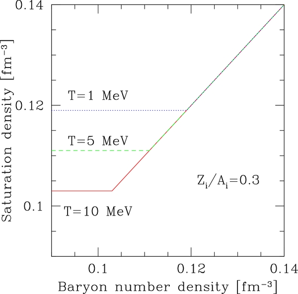
We define the saturation densities of nuclei nsi(T) as the baryon number density, at which the free energy per baryon, FRMF(T, nB, Yp), given by the RMF with Yp = Zi/Ai takes its minimum value. Thus, nsi(T) depends on the temperature T and the proton fraction in each nucleus Zi/Ai. At high temperatures the free energy, FRMF(T, nB, Zi/Ai), has no minimum because the entropy contribution, the TS term with S being entropy, overwhelms the internal energy. In the previous paper, nsi is set to the saturation density given by the H. Shen EOS at temperatures higher than the critical temperature Tci, above which the free energy, FRMF(T, nB, Zi/Ai), has no minimum. This prescription brought unphysical jumps in the mass fraction at the critical temperatures in the previous EOS. In order to remedy this artifact, we assume in the new EOS that the saturation density nsi(T) above Tci is equal to the saturation density at the critical temperature nsi(Tci). Figure 1 shows the saturation density nsi(T, Zi/Ai) for the proton fractions Zi/Ai = 0.2, 0.3, 0.4, and 0.5 in the nB–T plane. We can see that neutron-rich nuclei have lower saturation densities and critical temperatures than symmetric nuclei because of the symmetry energy. When the saturation density nsi is lower than the baryon number density of the whole system nB, we reset the saturation density as the baryon number density nsi = nB as shown in Figure 2. This prescription approximately represents compressions of nuclei near the saturation densities. These treatments of the saturation density are important in obtaining reasonable bulk energies at high temperatures and densities. They are necessary, since it is impossible at the moment to solve nuclear structures and abundance in a self-consistent manner completely. In fact, the density of each nucleus is not a quantity to be determined by the minimization of the free energy density but a parameter to be set in our model. We expect, however, that the density of each nucleus is very close to the saturation density, that is, the density at which the free energy density of uniform nuclear matter becomes minimum for the same temperature and proton fraction except when the saturation density does not exist at high temperatures or when the transition to uniform nuclear matter occurs at a density higher than the saturation density. To these cases we need special cares as described above.

Figure 1. Saturation densities of nuclei as a function of temperature for Zi/Ai = 0.2 (cyan dotted line), 0.3 (blue dash-dotted line), 0.4 (green dashed line), and 0.5 (red solid line).
Download figure:
Standard image High-resolution image
Figure 2. Saturation densities of nuclei with Zi/Ai = 0.3 as a function of baryon number density for T = 1 MeV (blue dotted line), 5 MeV (green dashed line), and 10 MeV (red solid line).
Download figure:
Standard image High-resolution image2.1.1. Coulomb and Surface Energies
To calculate the Coulomb and surface energies of nuclei we set the Wigner–Seitz cell (W–S cell) for each species of nuclei so that the charge neutrality could be satisfied. Each nucleus is centered in the W–S cell with the volume, Vi. The cell also contains free nucleons as a vapor outside the nucleus as well as electrons, which are assumed to be uniform in the entire cell. The charge neutrality in the cell gives the cell volume  where
where  is the volume of the nucleus in the cell and can be calculated as
  . The vapor volume and nucleus volume fraction in the cell are given by
  and
and  , respectively.
In this EOS, we assume that each nucleus enters the nuclear pasta phase individually when the volume fraction, ui, reaches 0.3 and that the bubble shape is realized when it exceeds 0.7 (Watanabe et al. 2005). The bubbles are explicitly treated as nuclei of spherical shell shapes with the vapor nucleons filling the inside. This phase is important to ensure continuous transitions to uniform matter as noted in Furusawa et al. (2011). The intermediate states (0.3 < ui < 0.7) are smoothly interpolated from the normal and bubble states. The criterion of intermediate states (0.3 < ui < 0.7) is admittedly rather arbitrary, although we consulted the literature (Watanabe et al. 2005) in adopting these numbers. We have hence tried another choice, 0.4 < ui < 0.6, and confirmed that the thermodynamic quantities are hardly affected. On the other hand, the nuclear composition is rather sensitive to the criterion particularly when the temperature is low and most of the nuclei form pastas simultaneously, since the surface and Coulomb energies are modified. Since the density region that corresponds to the intermediate states is narrow and the sums of Coulomb and surface energies for the drop and bubble states are equal to each other at ui = 0.5, the inclusion of the intermediate phase is mainly meant to ensure the smooth change in mass fractions of nuclei around ui = 0.5. The evaluation of the Coulomb energy in the W–S cell is given by the integration of Coulomb forces in the cell:

with  , where e is the elementary charge.
The surface energy of nuclei is given by the product of the nuclear surface area and the surface tension:


where  and
and  are the radii of nucleus and bubble. σ0 denotes the surface tension for symmetric nuclei. The surface tension σi includes the surface symmetry energy, i.e., neutron-rich nuclei have lower surface tensions than symmetric nuclei. The values of the constants, σ0 = 1.15 MeV fm−3 and Ss = 45.8 MeV, are adopted from the paper by Lattimer & Swesty (1991). The appropriate estimation of surface tensions is important, since they have a critical influence on the abundance of nuclei and, as a consequence, on the average mass number of nuclei, as shown in Buyukcizmeci et al. (2013a). We may choose other values such as those given in Lee & Mekjian (2010), which include high-order temperature dependences. We prefer the simpler estimate by Lattimer & Swesty (1991) in this work, considering insufficient experimental information on the heavy and/or neutron-rich nuclei that exist in the supernova matter. The last factor in Equation (5),
  , is assumed to take into account the effect that the surface energy should be reduced as the density contrast decreases between the nucleus and the nucleon vapor. We use cubic polynomials of ui for interpolation between the droplet and bubble phases. The four coefficients of the polynomials are determined by the condition that the Coulomb and surface energies are continuous and smooth as a function of ui at ui = 0.3 and ui = 0.7.
2.1.2. Bulk and Shell Energies
We derive the bulk energies from the free energy per baryon of the uniform nuclear matter at the saturation density nsi for the given temperature T and proton fraction inside the nuclei Zi/Ai as

where FRMF(nB, T, Yp) is the free energy per baryon given by the RMF, which is the same as that for the free energy density of free nucleons. Note that this bulk energy includes the symmetry energy of nuclei. In the previous paper, Equation (7) is applied only to the nuclei with no experimental mass data. For the nuclei with experimental mass data available, on the other hand, the bulk energies are calculated as ![$E_{i}^{B+{\rm sh}} =M_i^{{\rm data}}-[E_i^C+E_i^{Su}]_{{\rm vacuum}}$](https://content.cld.iop.org/journals/0004-637X/772/2/95/revision1/apj475929ieqn24.gif) including the nuclear shell energies. Then they have no temperature dependence. In this paper, we evaluate the bulk energies of all heavy nuclei by Equation (7) so that the bulk energies of all nuclei would depend on the temperature.
including the nuclear shell energies. Then they have no temperature dependence. In this paper, we evaluate the bulk energies of all heavy nuclei by Equation (7) so that the bulk energies of all nuclei would depend on the temperature.
We include the shell effects separately in the mass formula of nuclei by using both experimental and theoretical mass data (Audi et al. 2003; Koura et al. 2005) to better reproduce the ordinary NSE EOS results in the low-density regime. The regions, in which the experimental and theoretical mass data are available, are shown in the nuclear chart in Figure 3. The shell energies are obtained from the experimental or theoretical mass data by subtracting our liquid drop mass formula, which does not include the shell effects  in the vacuum limit as
 ![$E_{i}^{{\rm Sh}} =M_i^{{\rm data}} -[ M_i^{{\rm LDM}} ]_{{\rm vacuum}}$](https://content.cld.iop.org/journals/0004-637X/772/2/95/revision1/apj475929ieqn26.gif) . The vacuum limit means that the nucleus is cold and isolated:
. The vacuum limit means that the nucleus is cold and isolated:  . At high densities, the shell effect of nuclei estimated in vacuum is considered to be diminished because of the existence of electrons, free nucleons, and other nuclei. We take this effect into account phenomenologically as follows:

where ρ0 is taken to be mB times the saturation density of symmetric nuclei nsi(T, Zi/Ai = 0.5) at temperature T. The last factor (ρ0 − ρ)/(ρ0 − 1012 g cm−3) accounts for the decay of shell effects at high densities. The choice of the critical density 1012 g cm−3 is rather arbitrary, since the dependence of shell energies on the density of ambient matter has not been thoroughly investigated yet. It is noted, however, that the structure of nuclei is known to be affected by ambient matter at these densities. The abundances of nuclei with magic numbers of protons or neutrons are affected by the shell energy and hence by the choice of the critical density. We have confirmed, however, that thermodynamics quantities are hardly changed for the critical density of 1013 g cm−3. The linear interpolation in Equation (8) makes the free energy not smooth and the pressure discontinuous at the boundaries of the interpolation region. In practice, however, the variation of the shell energy is quite minor compared with those of Coulomb and translational energies, and the discontinuities of the pressure are negligible.

Figure 3. Regions of experimental mass data from Audi et al. (2003) (black), theoretical mass data from Koura et al. (2005) (dark gray), and the nuclei calculated by LDM with no shell effects (light gray). The upper limits of proton and neutron numbers are 1000.
Download figure:
Standard image High-resolution imageWe neglect the shell energies of the heavy or neutron-rich nuclei with no available mass data, since we have no guidance to estimate the shell energy and such nuclei are abundant only at very high densities, where the shell effects will be minor anyway.
We sum up all the contributions to have the masses of heavy nuclei as  . For the nuclei with mass data available, this formula can be transformed to

where ΔEi means the difference from the vacuum limit: ΔEi = Ei − [Ei]vacuum. In the limit of low densities and temperatures, Mi is reduced to the mass data  . This feature is important for reproducing the ordinary NSE results in these limits (Timmes & Arnett 1999). At the saturation density, on the other hand, only the bulk energies
  survive, since other terms are diminished as the density approaches the saturation density in our model.
2.2. Mass Evaluation of Light Nuclei (Z ⩽ 5)
In this subsection, we explain how to evaluate the masses of light nuclei (Z ⩽ 5). Note that the mass formula employed for heavy nuclei, which is based on LDM, is inappropriate for light nuclei as already noted. We assume the descriptions of d, t, h, and α in dense and hot matter based on quasi-particles outside heavy nuclei, and no pasta phase is considered for them. The saturation densities of the four light nuclei are set to the constant value, 0.15 fm−3, in contrast to those of heavy nuclei, which depend on temperatures and densities. For the light nuclei (Z ⩽ 5) other than d, t, h, and α such as 7Li, we adopt the mass data with density and temperature corrections that are based on the LDM slightly different from that of heavy nuclei (see below for details).
The masses of d, t, h, and α are given by the following expression:

where  is the Pauli energy shift by other baryons,
  is the self-energy shift of the nucleons composing the light nuclei, and
  is the Coulomb energy shift.
For the Pauli energy shifts of the light nuclei, we employ the empirical formulae provided by Typel et al. (2010), which are quadratic functions fitted to the result of quantum-statistical calculations (Röpke 2009). Röpke investigated the binding energies of light clusters in hot and dense matter (T ≲ 20 MeV and nB ≲ 0.16 fm−3) by using the quantum-statistical approach. They regard the light clusters d, t, h, and α as quasi-particles and solve the in-medium Schördinger equation perturbatively. For the potential terms in pair interactions, Jastrow and Gaussian wavefunction approximations are adopted for d and others (t, h, α), respectively. Note that the fitting formulae of  in Röpke (2009) are obtained under the assumption that matter is composed of only nucleons and light clusters (Z ⩽ 2 and N ⩽ 2), which is not completely consistent with the situations of our interest, in which heavier nuclei are also existent. To obtain the Pauli energy shifts, we define the local proton and neutron number densities including light nuclei as


where η stands for the volume fraction (V − VN)/V. Then the Pauli energy shift  is given by the following expression:

which is quadratic in  . The density scale for the dissolution of each light nucleus is given by
  with the binding energy in vacuum,
  . The function δBj(T) represents the temperature dependence of the Pauli energy shifts and is originally derived with the Jastrow and Gaussian wavefunction approximations for d and other light nuclei, respectively, as

with yj = 1 + aj, 2/T. The parameters aj/1, aj/2, and aj/3 are given in Table 1.
Table 1. Parameters for the Quantum Approach
| Cluster j | aj, 1 | aj, 2 | aj, 3 | sj |
|---|---|---|---|---|
| (MeV5/2 fm3) | (MeV) | |||
| d | 38386.4 | 22.5204 | 0.2223 | 11.147 |
| t | 69516.2 | 7.49232 | ⋅⋅⋅ | 24.575 |
| h | 58442.5 | 6.07718 | ⋅⋅⋅ | 20.075 |
| α | 164371 | 10.6701 | ⋅⋅⋅ | 49.868 |
Download table as: ASCIITypeset image
The self-energy shifts of light nuclei are the sum of the self-energy shifts of individual nucleons composing the light nuclei  and the contribution from their effective masses
  :
:

where  with Σ0 and Σ being the vector and scalar potentials of nucleons. The effective mass contributions are given as
  with
with  . The coefficients sj for d, t, h, and α are given in Table 1. The potentials Σ0 and Σ are calculated from the RMF employed for free nucleons in this paper. Note that the coefficients sj are provided based on a different RMF theory with density-dependent meson–nucleon couplings (Typel 2005). However, the inconsistency should have little influence, since the effective mass term is in general smaller than the other two potential terms and the light nuclei are not abundant at high densities, where the effective mass terms could be large, due to the Pauli energy shifts and pasta formations of heavy nuclei.
More detailed explanations of the Pauli- and self-energy shifts are provided in Typel et al. (2010). Note that we neglect the dependence of the Pauli energy shifts on the momentum of the light clusters and that of the self-energy shifts on the momentum of nucleons composing the light clusters for simplicity.
The Coulomb energy shifts are calculated as


Although the evaluation of the Coulomb energy is identical to that for heavy nuclei in the droplet phase, the shifts are negligible compared with other energies. We do not take into account the nuclear pasta phases and surface energy shifts for the light nuclei.
The light nuclei (Zj ⩽ 5) other than d, t, h, and α are described by an LDM. Since the masses of light nuclei d, t, h, and α are almost unchanged at low densities, the Pauli- and self-energy shifts are negligible at low densities. Therefore, we assume that the temperature dependence of other light nuclei is not so strong at low densities either and the temperature dependence is important only at ρ > 1012 g cm−3, which are approximated as

where  is the surface energy shift, which is too small to make any difference except in the pasta phases. The self-energy shift is linearly interpolated between the bulk and shell energies in vacuum limit, which are estimated from the experimental mass data by subtracting surface and Coulomb energies in vacuum limit, and the self-energy of uniform matter obtained by the RMF theory. The Pauli energy shifts are neglected for these light nuclei, since no fitting formula is available. We assume that they experience the pasta phases in the same way as heavy nuclei. The Coulomb and surface energy shifts are calculated from the same LDM for heavy nuclei. We note that the light nuclei other than d, t, h, and α are not so important because they are never abundant under NSE, since d, t, h, and α are dominant over the other light nuclei at high temperatures and/or low densities, whereas heavy nuclei prevail in the opposite situations.
In our models, d, t, h, and α are treated as independent particles and they coexist with free nucleons outside heavy nuclei. At low densities, the masses of the light nuclei approach the experimentally known values, since the  ,
,  , and
, and  vanish in this limit. Near the saturation densities, light nuclei no longer exist because of the Pauli energy shifts and free nucleons and heavy nuclei in the pasta phases are abundant.
2.3. Translational Energies of Nuclei
The translational energy of nucleus i in our model free energy is based on that for the ideal Maxwell–Boltzmann gas and given by

where kB is the Boltzmann constant, nQi = (Mi/jkBT/2πℏ2)3/2, and  is the spin degree of freedom of the ground state. Note that the contribution of the excited states to free energy is encapsulated in the temperature dependence of the bulk energy. In the previous paper, we employed a functional form of gi(T) for the internal degree of freedom in Equation (19). The last factor on the right-hand side of Equation (19) takes account of the excluded-volume effect: each nucleus can move in the space that is not occupied by other nuclei and free nucleons. The factor reduces the translational energy at high densities and is important to ensure the continuous transition to uniform nuclear matter. The present form of the factor, (1 − nB/ns) = (V − Vbaryon)/V, gives a linear suppression in terms of the occupied volume Vbaryon and we always employ the nuclear saturation density for symmetric nuclei
 ![$n_s=\left[ n_{{\rm si}}(Z_i/A_i,T) \right] _{Z_i/A_i=0.5}$](https://content.cld.iop.org/journals/0004-637X/772/2/95/revision1/apj475929ieqn49.gif) for numerical convenience.
for numerical convenience.
2.4. Thermodynamical Quantities
After minimization, we obtain the free energy density together with the abundances of all nuclei and free nucleons as a function of ρB, T, and Yp. Other physical quantities are derived by partial differentiations of the free energy density. In so doing, all the terms concerning the excluded volume effects and the interpolation factors are properly taken into account to ensure the thermodynamical consistency as described in Furusawa et al. (2011) in detail. The baryonic pressure, for example, is obtained by the differentiation with respect to the baryonic density as follows:


where  is the contribution of the nucleons in the vapor; both
  and
and  come from the translational energy of nuclei in the free energy;
  ,
,  , and
, and  originate from the shell, Coulomb, and surface energies of nuclei in the free energy, respectively;
  and
and  are derived from the Pauli- and self-energy shifts of the light nuclei.
The entropy per baryon is calculated from the following expression:

This form is the same as that of the previous EOS. The partial derivative of the masses, ∂Mi, j/∂T, is originated from the temperature dependence of nuclear mass in the current formulation and given as follows:


where the entropy per baryon  is predicted by the RMF. The contribution of this term is normally negligible except near the nuclear saturation density.
3. RESULT
In this paper, we construct the EOS modifying the previous one (Furusawa et al. 2011). First, we focus on the changes for heavy nuclei, i.e., the employment of the theoretical mass data and the modification of the temperature dependences of the bulk energies and the internal degrees of freedom. Then we compare the results of the different modelings of the light nuclei Z ⩽ 5. We list five calculated models in Table 2.
Table 2. Different Models for Comparisons
| Model | Heavy Nuclei | Mass Data | Light Nuclei |
|---|---|---|---|
| 0a | Old LDM | Audi 2003 | Old LDM |
| 1a | LDM | Audi 2003 | LDM |
| 2a | LDM | Audi 2003 & KTUY2005 | LDM |
| 2b | LDM | Audi 2003 & KTUY2005 | Quantum approach |
| 2c | LDM | Audi 2003 & KTUY2005 | Mass data |
Notes. Model 0a is the same EOS as Furusawa et al. (2011). The new model of heavy nuclei of Models 1a, 2a, 2b, and 2c is explained in Section 2.1. Audi 2003 and KTUY2003 are the experimental and theoretical mass data, respectively. The quantum approach of light nuclei is described in Section 2.2.
Download table as: ASCIITypeset image
Model 0a is nothing but the previous EOS except for the assumption on the saturation densities: in the previous one, the saturation densities at high temperature are determined by H. Shen EOS, whereas in the new models, they are derived from the RMF calculation as noted in Section 2.1. In Model 0a, the temperature dependence of the bulk energies of the nuclei, for which the mass data are available, is neglected and the bulk energies including the shell energies are derived from the experimental mass minus the Coulomb and surface energies in vacuum as

To take into account the excited states at high temperatures, the temperature dependence is introduced in  in Equation (19). The functional form is adopted from Fai & Randrup (1982) as

in which  MeV−1, c1 = 0.2 MeV−1, and c2 = 0.8. More details about the bulk and shell energies
  as well as gi(T) are found in Furusawa et al. (2011).
In the new Models 1a, 2a, 2b, and 2c, we employ the temperature-dependent bulk energies  in Equation (7) instead of Equation (29). The difference between the two treatments is most clearly presented as follows: the number density ni of heavy nucleus i depends on the internal degree of freedom gi(T) and the mass energy Mi(T) as ni∝gi(T)exp (− Mi(0)/T) in Model 0a, and ni∝gi(0)exp (− Mi(T)/T) in the other Models 1a, 2a, 2b, and 2c. This leads us to introduce the effective internal degree of freedom
  to express the number density as
  . This
  is in general much larger than gi(T). In fact the ratio,
  , for 56Fe is 9.18, 75.9, and 130 at T = 1, 5, and 10 MeV, respectively. For the nuclei with no available experimental mass data in Model 0a, the bulk energies are calculated from Equation (7) and, as a result, both the bulk energies
  and the internal degrees of freedom gi(T) depend on the temperature. This double count of the excited states leads to the overestimation of abundances of this type of nuclei as shown later.
The bulk energies in Model 1a are all derived from the RMF calculations with the temperature dependence included as described in Section 2.1. We consider that Model 2a is the most realistic model for heavy nuclei. We utilize the theoretical mass data by Koura et al. (2005) in addition to the experimental mass data in the calculation of the shell energies. Models 0a and 1a include only experimental mass data by Audi et al. (2003), on the other hand. Note that we neglect the shell energies for the nuclei with no mass data available and that the maximum of proton and neutron numbers is set to 1000 in all models.
In Models 0a, 1a, and 2a, the binding energies of light nuclei are evaluated from the LDM employed for heavy nuclei. Model 2b is modified from Model 2a only in the mass evaluation of the light nuclei with Z ⩽ 5. The LDM for heavy nuclei and mass data are identical to those in Model 2a. The masses of the light nuclei in Model 2b are based on the quantum approach, the details of which are given in Section 2.2. To examine the effect of the Pauli- and self-energy shifts, we prepare Model 2c, in which they are set to ΔEPa = ΔESE = 0. This means that the masses of d, t, h, and α are evaluated as  in Model 2c. We consider that Model 2b is the best among all five models.
3.1. Abundances of Heavy Nuclei
The mass fractions of nuclei for Models 0a and 2a are shown in the (N, Z)-plane for ρB = 1012 g cm−3, T = 1 MeV, and Yp = 0.3 in Figures 4 and 5. We can clearly see the gap between the nuclei with the experimental mass data and those without them in Figure 4. On the other hand, there is no such gap in Figure 5, since the range of the nuclei, for which the shell energies are included, is expanded to N ∼ 200 by the use of theoretical mass data. In Model 2a, the mass fractions of the nuclei in the vicinities of the magic numbers N = 50 and 82 are enhanced and, as a result, the fractions of other nuclei, in particular those with N ∼ 20, in 2a are smaller. This effect can be seen also in the isotope abundance discussed in the next paragraph.

Figure 4. Mass fractions in log10 of nuclei in the (N, Z)-plane for Model 0a at ρB = 1012 g cm−3, T = 1 MeV, and Yp = 0.3.
Download figure:
Standard image High-resolution image
Figure 5. Mass fractions in log10 of nuclei in the (N, Z)-plane for Model 2a at ρB = 1012 g cm−3, T = 1 MeV, and Yp = 0.3.
Download figure:
Standard image High-resolution imageThe isotope abundances of the nuclei with Z = 26 are shown for two combinations of temperature and baryon density in Figure 6. The main difference between Model 2a and the others manifests in the range of 74 ⩽ A ⩽ 99. For the nuclei with Z = 26, the experimental mass data are available only for 45 ⩽ A ⩽ 73, whereas the theoretical mass data cover the range of 44 ⩽ A ⩽ 99. Note that the theoretical mass data are not employed in Models 1a and 0a. We can see unphysical jumps in the abundance at the boundary between A = 73 and 74 for Models 1a and 0a in Figure 6. The difference between Models 1a and 0a, on the other hand, arises from the different treatments of the bulk energies for the nuclei with the experimental mass data as well as of the internal degrees of freedom. Note that the bulk energies including the temperature dependence given by Equation (7) tend to be lower at non-vanishing temperatures, since hot nuclear matter has lower free energies than a cold one due to excitations of nucleons. In other words, hot nuclei are more bound than cold ones owing to the increases in the internal degrees of freedom of the nucleons inside nuclei. The nuclei with 45 ⩽ A ⩽ 73 in Model 0a, for which the experimental mass data are available, have larger mass energies than the counterparts in Model 1a, since the bulk energies of these nuclei in the former do not include the temperature dependence. As a result, those nuclei are more abundant in Model 1a. On the other hand, the mass fractions of the nuclei with no experimental mass data (A ⩾ 74) in Model 0a are larger than in Model 1a due to the double count of the temperature effect in the bulk energies  and internal degrees of freedom gi(T). The difference between Models 0a and 1a is clear at higher temperatures, since the temperature dependences in the bulk energies and internal degrees of freedom become stronger. We can also find that Model 2a does not produce the unphysical jumps in the abundances at both low and high temperatures owing to the modified treatment of the temperature effects as well as to the employment of the theoretical mass data.

Figure 6. Isotope abundance of the nuclei with proton number Z = 26 for Models 0a (blue dotted lines), 1a (magenta dash–dotted lines), and 2a (green dashed lines) at (ρB = 1012 g cm−3, T = 1 MeV, Yp = 0.3) and (ρB = 1013 g cm−3, T = 5 MeV, Yp = 0.3).
Download figure:
Standard image High-resolution imageThe average mass number of heavy nuclei (Z ⩾ 6) as a function of density for the temperatures (T = 1, 5, and 10 MeV) and proton fractions (Yp = 0.3 and 0.5) is displayed in Figure 7 for Models 0a, 1a, and 2a. It is found that for T = 1 MeV the average mass number grows stepwise for Model 2a even at high densities, ρB ≳ 1013 g cm−3. On the other hand, they grow monotonically in Models 0a and 1a at A ≳ 120. This is due to the lack of shell energies for the latter models. The nuclei in the vicinity of the neutron magic numbers (N = 28, 50, 82, 126, 184) are abundant in Model 2a. Note that the experimental mass data are available at the magic numbers N = 28, 50, 82 under this condition, whereas the mass data for the nuclei with N = 126 such as 208Pb exist only near the stable line as shown in Figure 3. We can see that at the high temperatures (T = 5, 10 MeV), Model 0a gives larger mass numbers than the other models. This is because the nuclei, for which the mass data are available, are not abundant due to the lack of the temperature dependence in the bulk energies and the heavier nuclei, for which the temperature dependence is taken into account but the shell effects are neglected, are abundant. This feature can be confirmed also in the bottom panel of Figure 6.

Figure 7. Average mass number of heavy nuclei with Z > 6 for Models 0a (blue dotted lines), 1a (magenta dash–dotted lines), and 2a (green dashed lines) as a function of density for T = 1, 5, 10 MeV and Yp = 0.3, 0.5.
Download figure:
Standard image High-resolution imageTo summarize, the extended mass data and the temperature dependence remove the unphysical jumps found at the boundary between the nuclei with available mass data and those without them, at high temperatures in our previous paper. Even at low temperatures the wider use of the shell energy affects the nuclear abundances.
3.2. Abundance of Light Nuclei
In order to compare different models of light nuclei, we employ the total mass fraction of deuteron, triton, helion, and alpha particles, Xd + Xt + Xh + Xα, for Models 2a, 2b, and 2c. The abundances of other light nuclei are not so large and will not be discussed in the following. Figure 8 shows the results for the temperatures (T = 1, 5, and 10 MeV) and proton fractions (Yp = 0.3 and 0.5). For T = 5 and 10 MeV, we can see that the mass fraction of the light elements reaches the maximum at the densities ρB ≳ 1012 g cm−3 in Model 2a. This is because the light nuclei in this model have low bulk energies, since they are calculated by the same LDM employed for heavy nuclei. We can also see that the light nuclei are still abundant near the saturation densities for T = 10 MeV due to the suppression of the surface energies of the light nuclei in the pasta phases as well as to the lack of the Pauli energy shifts. Note that we assume in Models 2b and 2c that the light nuclei are quasi-particles and do not form pastas. The mass fractions of the light nuclei of Models 2b and 2c are similar between Models 2b and 2c because we do not adopt the LDM, which has a strong temperature dependence in the bulk energy. The difference between Models 2b and 2c arises from the Pauli- and self-energy shifts. We can see that the Pauli energy shifts slightly suppress the light nuclei at T = 5 MeV and Yp = 0.5 in Model 2b, whereas the self-energy shifts make them more abundant at T = 10 MeV in Model 2b than in Model 2c. Unlike in Model 2a, the light nuclei disappear near the saturation densities at T = 10 MeV in these models, since not only the self-energy shifts but also the Pauli energy shifts tend to suppress them and free nucleons and heavy nuclei are dominant, forming pastas. For T = 1 MeV, the light nuclei dominate around ρB ∼ 109 g cm−3. Since the Pauli- and self-energy shifts and the temperature dependence of bulk energies are rather minor, the three models give almost the same abundance.

Figure 8. Mass fractions of light nuclei (d, t, h, α) for Models 2a (green dashed lines), 2b (red solid lines), and 2c (black dotted lines) as a function of density for T = 1, 5, 10 MeV and Yp = 0.3, 0.5.
Download figure:
Standard image High-resolution imageWe show the mass fraction of each light nucleus for Model 2b in Figure 9. For T = 10 MeV, we can see that deuterons are the most abundant and alpha particles are the least, since lighter particles have more entropies per baryon. At T = 5 MeV, deuterons still dominate. The alpha particles are also abundant, on the other hand, since the binding energy becomes also important in the minimization of the free energy density. Note that alpha particles have the largest binding energy per baryon among the light nuclei. Under the neutron-rich condition of Yp = 0.3, the fraction of tritons is larger than that of helions, whereas tritons and helions have almost the same abundance for the symmetric condition of Yp = 0.5. At the lower temperature of T = 1 MeV, though not shown in the figure, alpha particles are dominant among the light nuclei due to the greatest binding energy per baryon.

Figure 9. Mass fraction of each light nucleus for d (red solid lines), t (magenta dashed lines), h (green dash–dotted lines), and α (blue doted lines) in Model 2b as a function of density for T = 5, 10 MeV and Yp = 0.3, 0.5.
Download figure:
Standard image High-resolution imageWe think that the abundance of light nuclei in Model 2a is too large at high temperatures due to the systematic overestimation of the binding energies in the LDM. The Pauli- and self-energy shifts have influences on the light nuclei abundance at high temperatures (T ≳ 5 MeV). It is important that deuterons, tritons, and helions can be as abundant as the alpha particles, which are normally assumed to be the representative light nucleus and incorporated in the two standard EOSs (Lattimer & Swesty 1991; H. Shen et al. 1998a, 1998b, 2011).
3.3. Thermodynamical Quantities
We compare the thermodynamics quantities for Models 0a, 2a, and 2b. Model 1a is not presented because it is almost the same as Model 0a at low temperatures and Model 2a at high temperatures (T ⩾ 5 MeV).
Figure 10 shows the free energies per baryon as a function of density for the three combinations of temperature and proton fraction: (T = 1 MeV, Yp = 0.3), (T = 5 MeV, Yp = 0.5), and (T = 10 MeV, Yp = 0.3). For T = 1 MeV, Model 0a has the highest free energy due to the lack of theoretical mass data, which are also evident in Figures 4, 6, and 7. Model 0a neglects the shell energies of the nuclei, for which no experimental mass data are available, whereas Models 2a and 2b employ the theoretical mass data. The free energies per baryon are not so different at T = 1 MeV between Models 2a and 2b, because the binding energies of heavy nuclei are dominant at this low temperature. For T = 5 and 10 MeV, on the other hand, we find that Model 2a gives lower free energies than Model 2b. The difference originates from the fact that the light nuclei are more abundant in Model 2a than in Model 2b, since Model 2a gives lower bulk energies to light nuclei due to the strong temperature dependence as shown in Figure 8. Model 0a also gives lower free energies per baryon than Model 2b because of the double count of the temperature effects in the bulk energies  and internal degrees of freedom gi(T) of the nuclei, for which no experimental data exist.

Figure 10. Free energy per baryon for Models 0a (blue dotted lines), 2a (green dashed lines), and 2b (red solid lines) as a function of density for (T = 1 MeV, Yp = 0.3), (T = 5 MeV, Yp = 0.5), and (T = 10 MeV, Yp = 0.3) from top to bottom.
Download figure:
Standard image High-resolution imageThe pressure is shown as a function of density for three combinations of temperature and proton fraction, (T = 1 MeV, Yp = 0.3), (T = 5 MeV, Yp = 0.5), (T = 10 MeV, Yp = 0.3), in Figure 11. The three models agree with one another at low densities, ρB ≲ 1012 g cm−3. For T = 1 and 5 MeV, the baryonic pressure is negative when the Coulomb-energy contribution, which is negative owing to the attractive Coulomb interactions between protons inside nuclei and uniformly distributed electrons (the so-called Coulomb corrections), dominates over the other positive contributions. For T = 1 MeV, the density, at which the pressure drop occurs in Model 0a, is higher than in the other models. The average mass numbers are smaller in Model 0a as shown in Figure 7 due to the lack of theoretical mass data, and the pressure drop occurs at higher densities than the other models. The pressures are almost the same at T = 1 MeV between Models 2a and 2b, since the contribution of light nuclei is negligible at low temperatures. For T = 5 MeV, on the other hand, the density, at which the pressure drop occurs, is the lowest in Model 0a. This is because the average mass numbers are larger as shown in Figure 7. The density, at which the pressure drop occurs, is highest in Model 2b, since the abundance of light nuclei, which contributes positively to the pressure, is larger in Model 2a than in Models 0a and 2b as shown in Figure 8. At the even higher temperature of 10 MeV, the positive thermal pressures of free nucleons and nuclei are dominant. Model 2a gives a little higher pressure than Model 2b near the saturation density, since the light nuclei are most abundant in Model 2a as shown in Figure 8. For Model 2b the pressure is the highest at ρB ∼ 1013 g cm−3, because free nucleons are the most abundant among the three models.

Figure 11. Baryonic pressure for Models 0a (blue dotted lines), 2a (green dashed lines), and 2b (red solid lines) as a function of density for (T = 1 MeV, Yp = 0.3), (T = 5 MeV, Yp = 0.5), and (T = 10 MeV, Yp = 0.3) from top to bottom.
Download figure:
Standard image High-resolution imageThe entropy per baryon is displayed as a function of density for three combinations of temperature and proton fraction, (T = 1 MeV, Yp = 0.3), (T = 5 MeV, Yp = 0.3), (T = 10 MeV, Yp = 0.5), in Figure 12. For T = 1 MeV, the entropy per baryon is almost identical among the three models. For T = 5, 10 MeV, on the other hand, Model 2a has larger values than Models 0a and 2b at ρB ∼ 1012 g cm−3 owing to the larger population of light nuclei as shown in Figure 8. For T = 5 MeV, Model 0a has the highest entropy per baryon near the saturation density because of the double count of temperature effects for the heavy nuclei with no mass data.

Figure 12. Entropy per baryon for Models 0a (blue dotted lines), 2a (green dashed lines), and 2b (red solid lines) as a function of density for (T = 1 MeV, Yp = 0.3), (T = 5 MeV, Yp = 0.3), and (T = 10 MeV, Yp = 0.5) from top to bottom.
Download figure:
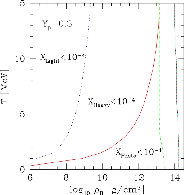
Standard image High-resolution image3.4. Phase Diagram
We finally discuss the phase diagram for Model 2b, which indicates the region where each of light, heavy, and pasta nuclei is an abundant boundary for the change of dominant composition. The boundaries are chosen so that each fraction of light, heavy, and pasta nuclei would be 10−4 following H. Shen et al. (1998a, 1998b). The total mass fraction of heavy nuclei is evaluated as  and that of light nuclei is
  , where X means the mass fraction. The mass fraction of the pasta nuclei XPasta is also calculated as

where ui is the volume fraction of nucleus i in its Wigner–Seitz cell. Note that d, t, h, and α are not included in this summation, since they are assumed not to form the pastas. In our EOS, the nuclei with ui ⩽ 0.3 are assumed to be normal, whereas those with 0.7 ⩽ ui < 1.0 are supposed to be bubbles and ui = 1.0 corresponds to the uniform matter. The nuclei with 0.3 < ui < 0.7 are interpolated between the droplets and bubbles, a very crude approximation to the rod, slab anti-rod phases. We can see in Figure 13 that the density range, in which heavy nuclei are abundant, becomes narrower as the temperature rises. This is because the entropy term −TS of free nucleons and light nuclei become more important than the internal energy term U of heavy nuclei in the free energy F = U − TS. Near the saturation densities, however, the pasta phase survives even at high temperatures, since it has almost the same free energies per nucleon as uniform matter. The abundance of pasta nuclei decreases and that of free nucleons increases monotonically as the temperature gets higher due to the small surface and Coulomb energies of the pasta phase.
Figure 13. Phase diagram of Model 2b at Yp = 0.3 in the ρB, T-plane. Blue dotted lines show the boundary where the light nuclei fraction (Z ⩽ 5) XL changes between XL < 10−4 and XL > 10−4. Red solid lines are that of heavy nuclei (Z ⩾ 6). Green dashed lines are that of pasta phase nuclei XPasta = ΣXi for pasta nuclei (ui > 0.3).
Download figure:
Standard image High-resolution image
4. SUMMARY AND DISCUSSIONS
We have extended the baryonic EOS at subnuclear densities, which was developed for the use in core-collapse supernova simulations in our previous paper. The EOS provides the abundance of various nuclei up to the proton number of 1000 in addition to thermodynamical quantities. The major modifications in the new EOS include the different treatments of the bulk and shell energies of heavy nuclei and the internal degrees of freedom, the use of the theoretical mass data wherever available, and the adoption of the different estimation of the masses of the light nuclei based on the quantum approach. The bulk energies of all heavy nuclei (Z ⩾ 6) now have the temperature dependence, which is different from the previous one. As a matter of fact, the temperature effects are encapsulated only in the internal degree of freedom of the nuclei, for which mass data are available, in the previous paper. In this paper, we employ the theoretical mass data in addition to the experimental ones to obtain the shell energies. For the light nuclei with Z ⩽ 2 and N ⩽ 2, the results of quantum calculations are adopted to better reproduce the binding energies of those nuclei at high densities and temperatures. For other light nuclei (Z ⩽ 5), we use the mass formula based on the LDM, which is different from the one for heavy nuclei. The LDM for the light nuclei gives a temperature dependence of the binding energies similar to that obtained from the quantum approach for Z ⩽ 2 and N ⩽ 2.
The basic part of the model free energy density is the same as that given in Furusawa et al. (2011). This model free energy density is constructed so that it should reproduce the ordinary NSE results at low densities and make a continuous transition to the supranuclear density EOS obtained from the RMF. For the nuclei with neither experimental nor theoretical mass data available, we have neglected the shell energies. At high densities, where the nuclear structure is affected by the presence of other nuclei, nucleons, and electrons, we have reduced by hand the shell energy from the value obtained from the experimental or theoretical data to zero at high densities. Assuming the charge neutrality in the W–S cell, we have calculated the Coulomb energy of nuclei. Close to the nuclear saturation density, the existence of the pasta phase has been taken into account in calculating the surface and Coulomb energies. The free energy density of the nucleon vapor outside nuclei is calculated by the RMF employed for the description of heavy nuclei.
For some representative combinations of density, temperature, and proton fraction, we have made a comparison of the abundances of nuclei as well as thermodynamical quantities obtained in different models. The model without the temperature dependence in the bulk energies for the nuclei with experimental mass data available (Model 0a) yields the unphysical jumps in isotope distributions, especially at high temperatures, because the bulk energies obtained from the RMF theory are lower than the experimental values. We have found that the introduction of the theoretical mass data solves this problem and changes the mass fractions as well as the average mass numbers. We have also revealed that the new EOS including the Pauli- and self-energy shifts gives lower abundances of the light nuclei than the old EOS based on the LDM. This is because the LDM overestimates the binding energies of the light nuclei at high temperatures. The Pauli and self-energy shifts also affect the light nuclei abundance at high temperatures and densities.
We would like to stress that the new EOS provides more realistic abundances of light and heavy nuclei than the previous one. In fact, the new EOS does not have undesirable jumps in the abundance of heavy nuclei. The mass estimation of light nuclei is also more sophisticated in the new EOS. We now briefly mention the comparison of our new EOS (Model 2b) with others. The detailed comparisons of our previous EOS (Model 0a) were made with EOSs employing SNA as well as with other multi-nuclei EOSs in Furusawa et al. (2011) and Buyukcizmeci et al. (2013a), respectively. It is found that the EOSs with SNA give mass numbers for the representative nuclei larger than the average mass numbers given by multi-nuclei EOSs such as ours. Furthermore, the two standard EOSs by Lattimer & Swesty (1991) and H. Shen et al. (2011) lack the shell energies of nuclei and, as a result, show monotonic growths of the average mass numbers of heavy nuclei, which are in contrast with our EOS, which gives stepwise growths as shown in Figure 7. As for light nuclei, we can provide their abundances in detail, whereas the two standard EOSs with SNA give only the abundance of alpha particles as the representative light nucleus. We have observed that at T = 5, 10 MeV the mass fractions of alpha particles given by H. Shen's EOS are larger than those in our EOS and are smaller than the total mass fractions of all light nuclei obtained in our EOS. This result implies that we cannot neglect deuterons, tritons, and helions and the replacement of the ensemble of light nuclei by alpha particles is a rather poor approximation at high temperatures.
Although we cannot compare our new EOS with other multi-nuclei EOSs, it is possible to infer that our new model (Model 2b) will give the mass fractions of heavy nuclei similar to those obtained in Botvina's EOS (Botvina & Mishustin 2004, 2010; Buyukcizmeci et al. 2013b) at high temperatures. This is because both EOSs take into account the temperature-dependent bulk energies for all heavy nuclei, as we have described in detail so far in this paper. There should be, of course, some differences, which could originate from the different estimations of the surface energies and inclusions of the shell energies, which are actually not taken into account in their EOS (Buyukcizmeci et al. 2013a). At low temperatures, the new EOS may give the abundances of heavy nuclei similar to those obtained by Hempel & Schaffner-Bielich (2010). This is because both EOSs include the shell effects for the neutron-rich and/or heavy nuclei by using theoretical estimations of nuclear masses. Note, however, that the difference between the theoretical mass data provided by Geng et al. (2005), which are used in Hempel & Schaffner-Bielich (2010), and those provided by Koura et al. (2005), which are adopted in this paper, may have some influences on the abundances of nuclei. As for the light nuclei abundances, we believe that our EOS has more reliable abundances than others, since ours takes into account the Pauli- and self-energy shifts, which could be important in medium. It is also pointed out that in Hempel's EOS, gi(T), the contribution from the internal degree of freedom to the nuclear partition function, is also applied to light nuclei with the integration range being somewhat limited despite the fact that deuterons have no excited states. Hemepl's EOS may hence overestimate the light nuclei abundance in some cases although they found no significant difference from the results in more involved calculations by Röpke (2009) and Typel et al. (2010) (Hempel et al. 2011). We infer from Furusawa et al. (2011) and Buyukcizmeci et al. (2013a) that thermodynamics quantities are not so different from different EOSs except at high densities, where the treatments of the pasta phase and abundances of light nuclei may make some differences.
There is room for improvement in our EOS. The interpolation of the shell energy and the treatment of the pasta phase are entirely phenomenological and need justification or sophistication somehow. We may have to improve the EOS of uniform matter, which is needed to evaluate the free energy density of the free nucleons and bulk energies of heavy nuclei. In fact, the RMF is known to have the symmetry energy larger than the canonical value, which will affect the neutron-richness, Zi/Ai, of heavy nuclei. In our formulation, however, it is quite simple to change the EOS of uniform nuclear matter, once it is provided. The combination with another EOS for supranuclear densities is indeed under progress at present. The update of the surface tensions of nuclei, especially of neutron-rich nuclei, should be considered according to the progresses in theories and experiments. The construction of the table based on Model 2b in this paper and its application to supernova simulations are also under way.
We gratefully acknowledge the contribution of A. Ohnishi and C. Ishizuka to the core idea. We thank H. Koura for useful data of the theoretical mass formula. S.F. thanks I. N. Mishustin, G. Martinez-Pinedo, S. Typel, and M. Hempel for their useful discussions. S.F. is grateful to FIAS for their generous support in Frankfurt. S.F. is supported by the Japan Society for the Promotion of Science Research Fellowship for Young Scientists. This work is partially supported by the Grant-in-Aid for Scientific Research on Innovative Areas (Nos. 20105004, 20105005, 24103006), the Grant-in-Aid for the Scientific Research (Nos. 19104006, 21540281, 22540296, 24244036), and the HPCI Strategic Program from the Ministry of Education, Culture, Sports, Science, and Technology (MEXT) in Japan. Part of the numerical calculations were carried out on SR16000 at YITP in Kyoto University. K.S. acknowledges the usage of the supercomputers at Research Center for Nuclear Physics (RCNP) in Osaka University, The University of Tokyo, Yukawa Institute for Theoretical Physics (YITP) in Kyoto University, and High Energy Accelerator Research Organization (KEK).