


ABSTRACT
We have used the continuous-time random-walk Monte Carlo technique to study the formation of H2 from two hydrogen atoms on the surface of interstellar dust grains with both physisorption and chemisorption sites on olivine and carbonaceous material. In our standard approach, atoms must first enter the physisorption site before chemisorption can occur. We have considered hydrogen atom mobility due to both thermal hopping and quantum mechanical tunneling. The temperature range between 5 K and 825 K has been explored for different incoming H fluxes representative of interstellar environments with atomic hydrogen number density ranging between 0.1 cm−3 and 100 cm−3 and dust grain sizes ranging from 100 sites to 106 sites, the latter corresponding roughly to olivine grains of radius 0.2 μm. In addition, we have also considered rough surfaces with multiple binding sites. Tunneling is found to dominate the surface chemistry at low temperature, but as the temperature increases, the scenario changes. The inclusion of chemisorption sites can provide a meaningful efficiency for H2 production up to temperatures as high as 700 K depending upon the depth of the chemisorption well. We found that over virtually the entire temperature range studied, the use of rate equations overestimates the H2 formation rate to some extent. This overestimate is large at high temperatures, due to very low surface residence times. We have also considered models in which chemisorption sites are entered directly and diffusion proceeds only to other chemisorption sites.
Export citation and abstract BibTeX RIS
1. INTRODUCTION
Molecular hydrogen (H2) is a critical molecule in the interstellar medium (ISM). Almost all of the elemental hydrogen in translucent and dense molecular clouds is in its molecular form, which is also the most abundant molecular species in diffuse clouds. Moreover, H2 is observed in large quantities in various galactic and extragalactic sources such as photon-dominated regions (PDRs), jets, shocks, outflows of planetary nebula, active galactic nuclei, and supernova remnants. In spite of its overwhelming presence, the process of H2 formation in these diverse environments is not entirely clear. Since H2 plays a crucial role in the dynamical and chemical evolution of the ISM, the study of how H2 is formed remains of fundamental importance.
Except in unusual environments such as pertained in the early universe (Kreckel et al. 2010), the gas-phase formation of H2 is inefficient and cannot account for the observed abundance of H2 (Gould & Salpeter 1963). Indeed, it is now well established that H2 forms on the surfaces of the interstellar dust grains. The dust provides a surface for hydrogen atoms to meet and react and also removes enough of the reaction exothermicity so as to stabilize H2 formation. In the last few decades, the formation of H2 in the ISM has been studied in extensive detail, both theoretically (Gould & Salpeter 1963; Hollenbach & Salpeter 1970, 1971; Hollenbach et al. 1971; Smoluchowski 1981, 1983; Aronowitz & Chang 1985; Duley & Williams 1986; Farebrother et al. 1999; Biham et al. 2001; Green et al. 2001; Chang et al. 2005, 2006; Acharyya et al. 2005; Chakrabarti et al. 2006) and experimentally (Brackmann & Fite 1961; Schutte et al. 1976; Pirronello & Averna 1988; Pirronello et al. 1997a, 1997b, 1999; Manicò et al. 2001; Hornekær et al. 2003; Roser et al. 2002, 2003).
The experiments performed by Pirronello et al. (1997a, 1997b, 1999) and analyzed by Katz et al. (1999) produced the first experimental data for use in astrochemical models. In particular, they determined the binding energies for hopping and desorption of H atoms on silicate (olivine) and carbonaceous surfaces, which are believed to be close analogs of bare interstellar dust grains. The binding was found to be weak, a situation known as physisorption. In addition, they did not obtain any evidence of quantum mechanical tunneling by H atoms on the surfaces used, which had earlier been thought to be the cause for hydrogen mobility on the grain surface (Hollenbach & Salpeter 1970). Instead they found that thermal hopping is the dominant physical process that provides mobility to adsorbed hydrogen atoms. They also found that by extrapolation of their model to astrophysically relevant conditions, the formation of H2 is efficient for flat olivine surfaces between 5 K and 8 K, while for amorphous carbon the efficiency is high between 8 K and 14 K. Slightly different results were obtained by Cuppen & Herbst (2005). Thus, a combination of both types of flat grains can explain H2 formation in the temperature range from ≈5–15 K. However, H2 formation beyond this temperature is frequently observed. In unshielded diffuse regions, in which the temperature of mid-sized grains is around 20 K (Li & Draine 2001) H2 is believed to form efficiently. In addition, dust grains smaller than 0.01 μm show temperature fluctuations due to interaction with UV radiation, which frequently heat the grains up to 40 K (Cuppen et al. 2006). In photodissociation regions (PDRs), the grain surface temperature can be above 75 K (Tielens & Hollenbach 1985a, 1985b), while in low-metal dwarf galaxies dust temperatures can reach 120 K (Hirashita et al. 2002). There are gas–grain models that posit the gas and grain temperatures to be equal so that even higher grain surface temperature can be considered. For example, Doty et al. (2004) considered the grain temperature of IRAS 16293−2422 to be around 250 K.
Several attempts have been made to explain how H2 formation can occur at surface temperatures beyond 15 K. First, by introducing grains with rough or amorphous surfaces, in which binding sites do not all have the same binding energy (Chang et al. 2005), Cuppen & Herbst (2005) were able to extend the temperature range of H2 formation up to 30–40 K depending upon whether the surface is a silicate or carbonaceous one. Indeed, more recent experiments by Perets et al. (2007) confirm the theoretical work, at least qualitatively. An earlier calculation of this type with similar conclusions had been performed by Hollenbach & Salpeter (1971). Second, one can consider H2 formation on surfaces that strongly support bound binding sites, known as chemisorption. The first attempt to use chemisorption to produce H2 under astronomical conditions was undertaken by Cazaux & Tielens (2002, 2004) and Cazaux et al. (2005). These authors found that chemisorption extends the upper temperature limit for efficient H2 formation considerably. More recent experiments of H2 formation on graphite by Hornekær et al. (2006) have shown that strong binding sites are an integral part of a rather complex process at higher temperatures. On the other hand, the role of quantum mechanical tunneling, if it does occur (Hollenbach et al. 1971), generally but not always appears to be more effective at extending the lower temperature limit of efficient H2 formation, as shall be seen below.
There are now several theoretical methods to study the surface chemistry that occurs on interstellar dust grains under a variety of astrophysical conditions. These approaches include the rate equation method, as well as several more detailed stochastic methods, based upon either the direction solution of the master equation or a Monte Carlo realization of this solution. The earliest studies were done with the standard rate equations used for diffusive reactions in surface science, which are based on average surface abundances, an approach most useful when there are large numbers of reactants on a given surface (Hasegawa et al. 1992; Biham et al. 2001). Given that grains are small particles and that the ISM is very dilute, the accretion rate of incoming species such as H atoms onto grains will be very low. As a result, at any instant of time the average number of a species such as atomic H on a single grain surface can be less than unity and the surface population of reacting species can fluctuate widely, which leads to an overestimation of the rate of H2 formation and the need for a stochastic approach (Charnley et al. 1997; Caselli et al. 1998; Shalabiea et al. 1998; Stantcheva et al. 2001). The departure from average values will be more severe the higher the temperature, because the residence time for H atoms on grains will decrease. Thus, at low flux and at high temperatures, the rate equation method is least likely to be successful.
Following work by Charnley (1998, 2001), Biham et al. (2001) and Green et al. (2001) proposed a direct master equation method independently and used it to study small systems of surface reactions: H2 recombination for Biham et al. (2001) and H2, O2, and OH formation for Green et al. (2001). In the master equation approach, surface abundances are calculated using the time evolution of coupled probabilities and one has to solve a large number of equations, ideally infinite. Several authors have used the master equation approach for a smaller system of surface reactions because the surface equations can easily be coupled to rate equations for the gas-phase chemistry (Stantcheva et al. 2001; Stantcheva & Herbst 2004; Acharyya et al. 2005). Even so, approximations are needed to render the approach more tractable for large-scale calculations: these include using the master equation only for reactive surface species of small abundance (Stantcheva & Herbst 2004; Acharyya et al. 2005) and using the method of moments (Barzel & Biham 2007). Although useful for H2 formation (Le Petit et al. 2009) and larger systems of surface equations, the latter approximation is still under development for systems coupled to gas-phase chemistry because of mathematical instabilities. Recently, so-called hybrid methods have been used to stabilize the moment equation approach (Du & Parise 2011).
The other approach is the Monte Carlo method, which can be used to simulate the direct master equation method for probabilities of surface abundances, but has the flaw, for gas–grain systems of reactions, that it is very difficult to couple to rate equations for gas-phase chemistry. The difficulty has been solved by Vasyunin et al. (2009), who developed a method to solve both the gas-phase and surface chemistry simultaneously using the Monte Carlo approach. The approach is computer intensive, and it is still difficult to solve the equations for periods of greater than 1 Myr. For smaller scale problems, such as the development of ice mantles or the formation of molecular hydrogen, a more detailed Monte Carlo approach, known as the continuous-time random-walk (CTRW) method, or more simply the kinetic Monte Carlo technique, is exceedingly useful (Cuppen et al. 2009). The advantage of this "microscopic" technique is that it treats all atoms and molecules individually, and monitors their moves (accretion, hopping, desorption, recombination) on the grain surface, treated as a lattice of binding sites, in a continuous time frame, which removes the error due to fluctuations in the populations of the species (Chang et al. 2005; Cuppen & Herbst 2005). In addition, the technique can be used for rough and even amorphous surfaces by assigning different energy parameters to individual sites, and can simulate several mechanisms of surface reactions besides the diffusive (Langmuir–Hinshelwood) one, including the Eley–Rideal mechanism, in which a gas-phase species lands directly on an adsorbate, and reactions within the gaps of porous ices. The technique has been used to look at the development of ice mantles (Cuppen & Herbst 2007; Cuppen et al. 2009) and probe details of H2 formation (Cazaux et al. 2005; Cuppen et al. 2006; Herbst & Cuppen 2006). Chakrabarti et al. (2006) used a similar method that keeps track of each individual reactant and their movements and calculated the effective grain surface area involved in the formation of molecular hydrogen in interstellar clouds. Most recently, the kinetic Monte Carlo method has been used to study the very complex formation of H2 on graphite, which involves preliminary dimer formation (Cuppen & Hornekaer 2008; Gavardi et al. 2009). An astronomical application of H2 formation in shocks, where the gas temperature is very high but the dust temperature quite low, has also been undertaken (Cuppen et al. 2010).
In this paper, we develop an overall picture of the efficiency of H2 formation on silicate and carbonaceous grains via the diffusive mechanism over a wide range of temperatures and other physical conditions with the use of the CTRW method and the corrected physisorption–chemisorption model of Cazaux & Tielens (2002, 2004, 2010). The results can be compared with those of Cazaux & Tielens (2002, 2004, 2010), in which rate equations are used, and with Cazaux et al. (2005), in which a brief report is given on the use of Monte Carlo methods. We consider routes via physisorption and chemisorption as well as via pure physisorption, on flat and rough surfaces, and via thermal hopping and tunneling. Such an overall picture gives a sense of how H2 is produced in widely differing interstellar environments, although the detail used is not as great as in simulations over more limited ranges (Cuppen & Hornekaer 2008). We are particularly interested in high temperatures since it is under these conditions that the detailed Monte Carlo results and the more widely used rate equation results are likely to differ most strongly (Cazaux et al. 2005).
2. PROCESSES ON GRAIN SURFACES
There are four physical processes that are involved while gas-phase atoms/molecules interact with the grains and undergo diffusive reactions. The first step is accretion; i.e., the landing of species onto a grain. In our case, H is the only species accreting onto the grain surface.
2.1. Accretion
With the assumption that sticking occurs on every collision with a grain, the accretion rate, or flux (fH), of H atoms onto the surface of a dust grain, in units of monolayer per second (ML s−1), is given by the equation

where nH and  are, respectively, the number density and average velocity of H atoms in the gas phase, and ns is the number density of sites on the surface of dust grain. The factor of four comes either from the assumed spherical shape of grains or from the average velocity normal to the surface. The expression for
  is
is

where m is the mass of H atoms and Tgas is the temperature of the hydrogen gas. The rate of accretion of H atoms onto the surface of a dust grain in units of atoms s−1 is given by

where σgr is the cross section of the spherical dust grain. The relation between the number of sites (Ns) on the grain surface and the grain cross section is

Using Equations (3) and (4), we obtain

which relates the accretion rate in ML s−1 and atoms s−1.
2.2. Hopping, Tunneling, and Desorption
Hydrogen atoms adsorbed on a grain site can move to another site via tunneling or hopping; the latter mechanism requires sufficient energy to overcome the energy barrier between the sites. We assume granular surfaces to be square lattices with four nearest neighbor sites, as on an fcc[1 0 0] plane, and that the probability of hopping or tunneling to each nearest site with the same barrier is the same. Different barriers occur between different pairs of sites, which can be sites in which H atoms are weakly bound, due to physisorption, or strongly bound, due to chemisorption. We imagine a surface on which physisorption and chemisorption sites occur at different heights and are offset horizontally from one another as well so as to form two offset planar lattices. Diffusion among chemisorption or physisorption sites occurs horizontally, while diffusion between the different types of sites has a vertical component as well. The assorted potentials and associated parameters are shown in Figures 1–3 of Cazaux & Tielens (2004). The physisorption sites must be entered first, corresponding to the well-known process of precursor-mediated adsorption in surface science (Kolasinski 2008).
Following Messiah (1999) and the corrected formula in Cazaux & Tielens (2010), for a species with energy E, the equations for the transmission coefficient (Tij) from site i to site j are given by
for tunneling and
for hopping. Here i and j can represent either physisorption (p) or chemisorption (c) sites, and Z is the width of the barrier. Expressions for Bij, Bi, Bj, and Z in terms of potential parameters for the four cases p-p, c-c, p-c, and c-p can be seen in the revised Table 1 of Cazaux & Tielens (2010). Based on the work of Cazaux & Tielens (2004), we utilized models O1, O2, and O3 for a flat olivine surface and C1, C2, and C3 for a flat carbon surface. The potential parameters for each model are shown in Table 1. In addition to parameters representing assorted heights for the potentials, there are parameters for potential widths (a for p-c and c-p and A for c-c and p-p). The three models differ in the following parameters: Model 1 is based on "typical physical characteristics of silicate and carbonaceous surfaces" (Cazaux & Tielens 2004), whereas the other models are based on fits by Cazaux & Tielens (2004) to both low- and high-temperature temperature-programmed desorption results (Pirronello et al. 1997a, 1997b, 1999; Zecho et al. 2002). In Model 2, the chemisorption binding energy is raised considerably to 30,000 K from the Model 1 values of 10,000 K (olivine) and 14,000 K (carbon) and the barrier against tunneling/hopping from one such site to another, defined as one-half of the chemisorption energy, is also raised. In Model 3, preferred by Cazaux & Tielens (2004), the Model 2 parameters are changed for the width of the c-p and p-c potential, for the physisorption energy, and for the barrier against physisorption to chemisorption conversion. Essentially, in going from Model 2 to Model 3, an increase in width is counterbalanced by a decrease in the barrier height.
Table 1. Potential Height and Width Parameters
| Surface | a | A | Ephys | Echem | Es | Esp | Esc |  |
μ | Model |
|---|---|---|---|---|---|---|---|---|---|---|
| (Å) | (Å) | (K) | (K) | (K) | (K) | (K) | (K) | |||
| Olivine | 2.5 | 2 | 400 | 10000 | 100 | 100 | 5000 | 300 | 0 | O1 |
| Carbon | 2.5 | 2 | 780 | 14000 | 100 | 100 | 7000 | 300 | 0 | C1 |
| Olivine | 2.5 | 2 | 400 | 30000 | 100 | 100 | 15000 | 300 | 0 | O2 |
| Carbon | 2.5 | 2 | 780 | 30000 | 100 | 100 | 15000 | 300 | 0 | C2 |
| Olivine | 3 | 2 | 660 | 30000 | 100 | 100 | 15000 | 300 | 0 | O3 |
| Carbon | 3 | 2 | 860 | 30000 | 330 | 100 | 15000 | 300 | 0 | C3 |
Download table as: ASCIITypeset image
Following Cazaux & Tielens (2004), we integrated the transmission coefficients numerically over the energies available to H adatoms to obtain thermalized probabilities Pij(T) to go from one site to another site via both tunneling and/or hopping, where T is the dust/surface temperature. We then calculated the mobility (s−1), or frequency of motion, of the thermalized adatom from site i to site j via

where νi, labeled the attempt rate or trial frequency, can be approximated by the expression

Here El is the depth of the well to which the species is bound at the site i, m is the mass of the adatom, and ns = 5 × 1013 cm−2 for amorphous carbon and 2 × 1014 cm−2 for olivine (Biham et al. 2001).
In Figure 1, we show the mobility for H adatoms on the surface of olivine dust grains (Model O1) due to thermal hopping (lines without symbols) and tunneling (lines with triangles) separately. Mobilities from a physisorption to a physisorption site, a physisorption to a chemisorption site, a chemisorption site to a physisorption site, and a chemisorption to a chemisorption site are designated by p-p, p-c, c-p, and c-c, respectively. It is evident from the plot that at low temperatures, the mobility due to tunneling for atomic H is greater than the mobility due to hopping. However, as the temperature is increased, the scenario changes; the p-p hopping rate is greater than the tunneling rate above 30 K, while for the p-c, c-p, and c-c transitions, this crossover temperature is 20 K, 80 K, and 100 K, respectively.

Figure 1. Mobility curves for H adatoms on olivine (Model O1). The lines without symbols are for mobility due to thermal hopping only whereas lines with triangles are for tunneling only.
Download figure:
Standard image High-resolution imageFigure 2 shows the total mobility of H adatoms due to thermal hopping and tunneling for Models 1, 2, and 3, and illustrates the strong negative effect of increasing the chemisorption binding energy Echem. The mobility of H atoms on the olivine grain models is higher than that on the carbon grain models for this reason. Differences exist among the various olivine and carbon models as well, due principally to the increase in the chemisorption binding energy between O1(C1) and O2, O3 (C2, C3), while differences between the O2(C2) and O3(C3) models are due to more subtle potential effects. The p-c results for H at the lowest temperatures are in qualitative agreement with those of Cazaux & Tielens (2004, see their Figure 4), obtained with a different formula that was later corrected (Cazaux & Tielens 2010).

Figure 2. Total mobility due to hopping and tunneling for O1, C1, O2, C2, O3, and C3 models.
Download figure:
Standard image High-resolution imageIn competition with mobility, the adsorbed atom can desorb from site i at a rate according to the standard formula

where T is the surface temperature and Ei is the desorption energy for site i corrected for zero-point energy. Because the desorption energy from a physisorption site is much lower than the desorption energy from a chemisorption site, when an atom hops/tunnels to the latter, it will remain there unless the temperature is rather high.
2.3. H2 Recombination and Formation Efficiency
When an H atom hops or tunnels to a pre-occupied site in either the physisorption or chemisorption lattice, H2 is formed. In addition, if an H-atom hops or tunnels from a physisorption site to a filled chemisorption site (or the reverse), H2 formation can also occur. There are two mechanisms for desorption of the H2 product: immediate release due to energy obtained from the exothermicity of reaction and thermal desorption. A parameter μ is defined such that a fraction 1 − μ of the newly formed H2 is immediately released into the gas. In their original analysis of H2 formation, based solely on physisorption, Katz et al. (1999) determined μ to be 0.33 and 0.413, respectively, for olivine and for amorphous carbon, while in their later chemisorption–physisorption analysis, Cazaux & Tielens (2004) used μ = 0. Here, we choose μ = 0.
We run the code, which is discussed in more detail below, until a quasi-steady state is reached in which the surface population of H atoms fluctuates around a constant value. The time to reach the quasi-steady state, which depends upon the temperature and the incoming flux of hydrogen atoms among other parameters, takes between 103 and 1010 s. The code is then run for a further time, which is at least twice the time that is required to achieve a quasi-steady state, so as to reduce the statistical noise. After the quasi-steady state has been reached initially, we keep a continuous count of the number of arriving H atoms and the number of H2 molecules formed to determine the recombination efficiency (η) by the expression
where  is the number of H2 formed after the steady state and NH is the number of H atoms deposited on the grain in that period of time. We have calculated the efficiency under a variety of different conditions, including temperature and flux, the size and chemical nature of the grain (olivine or amorphous carbon), and the degree of roughness of the surface.
3. PROCEDURE
We used the CTRW Monte Carlo method, sometimes referred to as a kinetic Monte Carlo approach. In this technique, atoms and molecules are treated individually and their surface motions (accretion, hopping/tunneling, desorption, recombination) take place on a lattice depending upon the values of random numbers called in a continuous time frame (Chang et al. 2005). In order to mimic the spherical grain structure, we assumed periodic boundary conditions; i.e., a species that leaves the lattice on one side enters back from the opposite side. During the simulation, H atoms are deposited onto physisorption sites on the grain lattice randomly, while allowing for the Langmuir rejection mechanism, by which incoming atoms cannot land on sites already occupied by another H atom or H2 molecule. The lattice positions are simulated by a square array G(k, l). The random site for a possible accretion is generated by random number (X, 0 < X < 1), which is multiplied by the total number of sites (Ns) on the lattice. The result (y) is divided by the number of columns in the square lattice and then the integer 1 is added to the integral value of the result, which gives the k of the array. To determine the other index l, we take the result of the MOD function of y with the number of rows in the lattice and then add 1 to the integer value of it, which gives us l. Whether the H atom sticks or is rejected, a waiting time (WTacc) is subsequently generated for the next accretion attempt of an H atom, assuming the accretion of H atoms to be a Poisson (memory-less) process (Chang et al. 2005). The waiting time for accretion is given by the following standard expression:

where X is another random number, 0 < X < 1, and RH is as defined in Equation (5). The clock is then moved up from the current time t to determine the time of the next attempted accretion via

When an H atom in position k, l, designated Hkl, moves to another site, designated k', l', another waiting time is calculated for its next move via
where αi is the total mobility of the H atom from the site where it is adsorbed, and Wi is the desorption rate at that site, defined in Equation (10). Here we assume that the mobility and desorption are also independent Poisson processes with the same type of waiting time distributions, so that we can add the rates of the processes to get the total rate (αi + Ri), which is then used to get the waiting time (Chang et al. 2005). When the time for the next move for any H atom comes, a random number (X) is generated to see if the H atom will travel to another site or desorb. If X < Wi/(αi + Wi) then the H atom will desorb, otherwise it will travel to another site. If it travels (via hopping or tunneling) then another random number must be generated to determine whether the destination is a similar site or a different site. For example, if the H atom lies on a physisorption site and the generated random number X < αpp/αp, where αpp is the mobility of H atoms from physisorption to physisorption site and αp = αpp + αpc is the total mobility, then the H atom will travel to a physisorption site; otherwise, it will travel to a chemisorption site.
After each event (accretion, travel, recombination, or desorption) we determine a new waiting time, recheck what event comes next, simulate the event at this new time, determine a new waiting time, etc., until the overall simulation ends.
To investigate differences in results from the use of the kinetic Monte Carlo approach and the rate equation approach of Cazaux & Tielens (2004), we simulated the formation of H2 using both methods and considering the same parameters. In the rate equation approach, we can write the time evolution in units of fractional monolayers for physisorbed hydrogen atoms ( ), chemisorbed hydrogen atoms (
 ), and molecular hydrogen (
 ) following Cazaux & Tielens (2004) as follows:


where F is the effective flux, which is a combination of the accretion term as described in Equation (5), and the rejection of hydrogen atoms on pre-occupied sites; the αi, j are the mobilities from one site to other; for example αp, p is the mobility from a physisorbed site to another (nearest-neighbor) physisorbed site; and Wi is the desorption rate for the ith species. There is no desorption term in Equation (17) because all of the produced H2 is desorbed immediately. Following integration, the efficiency of conversion to H2 can then be calculated as shown in Cazaux & Spaans (2004) and Cazaux & Tielens (2002).
4. RESULTS AND DISCUSSIONS
We use dust grains of different radii corresponding to different numbers of sites on the surface ranging from Ns = 10 × 10 to 1000 × 1000, with a surface site density (ns) of 2 × 1014 cm−2 for olivine and 5 × 1013 cm−2 for amorphous carbon (Biham et al. 2001). Thus, for olivine, the grain radius varies between 20 Å and 2000 Å (0.2 μm), and for amorphous carbon it varies between 40 Å and 4000 Å (0.4 μm). We vary the H-atom flux by changing the number density (nH) of H atoms in the gas phase between 0.1 cm−3 and 100 cm−3. We also explore the role of tunneling and surface roughness. For each simulation, we vary the grain temperature in the range 5–825 K if possible. In addition, we have run our model with only physisorption sites and compared the results with those in which chemisorption sites also exist.
4.1. The Efficiency of H2 Formation
Figure 3 shows the variation of molecular hydrogen formation efficiency as a function of temperature for all six models (O1, O2, O3, C1, C2, and C3), at a density for nH of 10 cm−3, which corresponds to a flux of  ML s−1 for olivine and
  ML s−1 for carbon. The solid lines are results from the kinetic Monte Carlo simulation, while the dashed lines are from the rate equation method (Cazaux & Tielens 2004). The basic reason for the relatively high H2 formation efficiency at higher temperatures for physisorption–chemisorption models compared with pure physisorption models is the higher binding energy for chemisorption, which enables chemisorption sites to retain H atoms on the grain up to much higher temperatures so that H2 formation can still occur. Nevertheless, it can be seen that for all six models that the efficiency calculated by the Monte Carlo simulation lies below that calculated with the use of rate equations at all but the lowest temperatures. This effect occurs because the rate equation method does not take into account fluctuations and utilizes average abundances. As a result, it overestimates the H2 formation efficiency by a negligible to small (factor of a few) amount at low temperatures but by a much larger amount at high temperatures. At high temperatures, the average population of H atoms on a grain is more likely to be less than unity, while the minimum number of H atoms needed on a grain to produce H2 is obviously two. For example in Model O1, the discrepancy factor becomes larger than an order of magnitude at 250 K, at which temperature the number of H atoms is unity on the 100 × 100 site grains studied (see Section 4.1.1 below). At lower temperatures, one must make a distinction between the overall coverage and the coverage of the physisorption layer, since diffusion of physisorbed atoms to filled physisorption or chemisorption sites becomes the dominant mechanism leading to reaction. The overall coverage exceeds one H atom per grain (10−2%), while the coverage in the reactive physisorption layer can be less than 1 per grain. The small discrepancy at the lowest temperatures is due to a very small abundance of physisorbed H atoms (⩽1 atom per grain) which provide all of the reactants at these temperatures. A previous Monte Carlo approach to H2 formation was reported briefly by Cazaux et al. (2005), who obtained little difference with the results from their rate equation approach, as shown in their Figure 3, although the authors stated that at still higher temperatures, a difference was to be expected, for the same reasons given here.

Figure 3. Recombination efficiency as a function of temperature for a flat surface with Ns = 100 × 100 and a constant density nH of 10 cm−3, which corresponds to a flux of  ML s−1 for olivine and
  ML s−1 for carbon. These parameters represent our standard models. Solid lines: kinetic Monte Carlo simulation; dashed lines: rate equation method.
Download figure:
Standard image High-resolution imageIn addition to this effect, one also sees that for both approaches the efficiency decreases with increasing temperature, mainly due to the increasing rate of H atom desorption. For Model O1, the efficiency calculated by our simulation drops to lower than 0.1 at 200 K, whereas with rate equations, it remains at 0.2 between 100 K and 300 K and then goes down very sharply. The trends for Model C1 are similar but are shifted to higher temperatures; here the Monte Carlo method shows a dropping efficiency of 0.05 at 350 K while the rate equation method shows a constant value of 0.3 between 100 K and 420 K before dropping sharply. In Models O2 and C2, with a much higher chemisorption well depth, the efficiency of H2 formation at 800 K remains as high as 0.1–0.2 with the rate equation approach, while our Monte Carlo simulations show that by 700 K, the efficiency is down to ≈0.01. We observe a similar trend for Model O3, whereas Model C3 is somewhat different; here the Monte Carlo efficiency is closer to that calculated from rate equations until 700 K before dropping sharply. This latter result, which is closest to that of Cazaux et al. (2005), arises from potential effects that produce a p-c rate larger than the p-p rate, which means that a physisorbed H atom has a greater probability to hop to a chemisorbed site than to a physisorbed site, although hopping still has to compete with desorption. This effect results in a greater H atom population in chemisorbed sites and a higher reaction efficiency.
4.1.1. Hopping versus Tunneling
In Figure 1, we see that the mobility of H adatoms on chemisorption sites for Model O1 is many orders of magnitude lower than the mobility on physisorption sites for both tunneling and thermal hopping through 300 K. For physisorption sites, the mobility due to tunneling dominates up to ≈20 K, and above 20 K thermal hopping dominates, while for chemisorption sites, the tunneling dominates up to ≈100 K, while above 100 K thermal hopping dominates. A similar situation occurs for the other models. How do the relative mobilities for tunneling and hopping translate into H2 recombination efficiency? Figure 4 shows the recombination efficiency for Model O1 as a function of temperature. In the presence of tunneling, the efficiency is higher up to ≈40 K, while above this temperature tunneling plays little role. At very low temperatures (<7 K), the efficiency goes down rapidly if only hopping is included; when tunneling is included, it remains constant at near unity.

Figure 4. Recombination efficiency as a function of grain temperature for Model O1, with Ns = 100 × 100, and flux =  ML s−1. The solid line shows the efficiency when both hopping and tunneling are included while the dashed line shows the efficiency when only hopping is considered.
Download figure:
Standard image High-resolution imageMore detail about what is happening can be obtained by looking at the H atom surface coverage in physisorption and chemisorption sites as a function of temperature for Model O1. Figure 5 shows the percentage site coverage (100 × the fractional number of monolayers) for H as a function of temperature both in the presence and absence of tunneling. In the absence of tunneling (hopping only), the very high coverage at temperatures below 8 K is mainly due to immobile H atoms locked in physisorption sites because hopping is inefficient. At ≈8 K, mobility increases and reactions begin to occur even in the absence of tunneling. By 10 K, the H-coverage starts to decrease very slowly and is almost constant at ≈5% until 100 K. This effect occurs because once the physisorbed H-atoms have enough mobility, a fraction of H-atoms are moved to chemisorption sites and remain there due to low mobility and a negligible desorption rate. While the coverage is dominated by chemisorbed H atoms, H2 formation occurs mainly via the hopping of physisorbed H atoms onto chemisorption sites filled with atomic hydrogen. When tunneling is included, the coverage is low at very low temperatures because of the higher efficiency of reaction, but rises to 5% by 30 K, when the coverage is once again dominated by chemisorbed H atoms. As temperatures rise above 100 K, chemisorbed adatoms become mobile (see Figure 1), which causes an increase in H2 production so that the H-atom coverage starts to decrease strongly again. However, at this temperature, desorption can still not occur from a chemisorption site, so that an almost constant 1% coverage starts as the temperature reaches 150 K. Around 200 K, the desorption of chemisorbed H atoms starts, hence the coverage begins to decrease yet again. Because there are no more binding sites with higher energy, the coverage goes down very rapidly. At these temperatures, the average number of H atoms on the binding sites becomes less than unity and the rate equation approximation becomes a poor one.

Figure 5. Percentage coverage as a function of temperature for O1 model shown in Figure 4.
Download figure:
Standard image High-resolution imageFor completeness, Figure 6 shows a coverage versus temperature plot for Models O2, O3, C2, and C3 in which both hopping and tunneling are included. It is clear that for Model C3, the coverage is always higher, so one expects the calculated efficiency to be much closer to the rate equation result, which is indeed the case.

Figure 6. Percentage coverage as a function of temperature for Models O2, O3, C2, and C3 with "standard" parameters as in Figures 3 and 4.
Download figure:
Standard image High-resolution image4.1.2. Flux and Size Dependence
Figure 7 shows the dependence of the recombination efficiency on flux (or H-atom density) for a dust grain with Ns = 100 × 100, when Model O1 is used. Within the density range nH = 10−1 to 102 cm−3, there are only two regions where a significant dependence exists. Otherwise, the increase in flux translates into a proportional increase in H2 production, so that the efficiency (if not the rate) stays the same. The first zone, with a weaker dependence, lies between 90 K and 120 K. The second zone lies above 200 K, when the desorption rate is very high. Under these conditions, a higher flux means a higher number of H atoms on the grain, hence the probability to form an H2 molecule is also higher. Figure 8 shows the percentage coverage plot, from which we see that in these zones, the greater the flux the greater the coverage.

Figure 7. H2 formation efficiency for different hydrogen atom densities using Model O1 considering both hopping and tunneling.
Download figure:
Standard image High-resolution image
Figure 8. Percentage coverage for models shown in Figure 7.
Download figure:
Standard image High-resolution imageIn Figure 9, we show efficiency plots with the O1 model of H2 formation for grains with different numbers of sites, Ns, which are related to the square of the radii. Here, we see that the recombination efficiency is almost independent of the number of sites except for temperatures above 210 K. Here the coverage of adatoms becomes very low, so that there are not more than one or two adatoms per grain at a time. The smaller the size of the grain, the greater the time separation between two incoming H atoms. The probability of having two hydrogen atoms simultaneously on the grain surface is lower for smaller grains, especially at such a high temperature, and the efficiency of H2 recombination is less. Thus, the smaller the grain, the lesser the probability to form H2.

Figure 9. Recombination efficiency plots of H2 formation using Model O1 for different numbers of sites on a grain, considering both hopping and tunneling.
Download figure:
Standard image High-resolution image4.1.3. Effect of Rough Surface
To examine the effect of a rough surface on the recombination efficiency, we have generated a simple rough surface that has five different physisorption binding energies depending on lateral bonds as prescribed by Chang et al. (2006). To this we add chemisorption sites, all with the same binding energy. In Figure 10, we show the recombination efficiency as a function of temperature for a regular (flat) surface and our rough surface. Figure 10(a) represents the efficiency for olivine when only physisorption sites are considered. The panel shows that incorporation of a rough surface broadens the temperature window for higher efficiency. This result is discussed by Chang et al. (2006) in more detail, although the rough surface has certain similarities to the addition of chemisorption sites to physisorption sites in an otherwise flat surface, which can be thought of as a quasi-rough surface with two different types of sites. Given this analogy, one expects that if Models 1 and 2, with physisorption and chemisorption sites, are roughened for physisorption, little additional effect will occur, because the chemisorption sites are so much deeper than the roughened physisorption sites. Indeed, panels (b) and (c) of Figure 10 show that there is little to no effect of a rough surface on Models O1 and O2, respectively. Moreover, it is clear that the addition of chemisorption sites has a much larger effect on the efficiency as a function of temperature than does the addition of roughness to physisorption.

Figure 10. Recombination efficiency as a function of temperature for both flat and rough surfaces. Panel (a) contains results for physisorption sites only, panel (b) contains results for Model O1, while panel (c) contains results for Model O2. Other parameters are the same as used for Figure 4.
Download figure:
Standard image High-resolution image4.1.4. Barrierless Direct Chemisorption
Although our calculations have been based on a joint physisorption–chemisorption model in which physisorption sites are the only entrance sites, there are some systems in which direct barrierless chemisorption can occur without a precursor. It should be noted, however, that experiments and calculations indicate that H atoms can chemisorb onto graphite and graphene only after surmounting a barrier of 0.2 eV (Jeloaica & Sidis 1999; Bachellerie et al. 2009; Ivanovskaya et al. 2010). Nevertheless, we consider a model for barrierless chemisorption in which only chemisorption sites are available, based on Models O1 and O2. The results are shown in Figure 11, where we can see that the efficiency with the O1 model lies near unity between 100 K and 250 K, dropping off sharply at lesser and greater temperatures. The efficiency for the O2 model follows a similar pattern except that it occurs at higher temperatures: the efficiency is near unity from 400 K through 750 K. These models with barrierless direct chemisorption yield high efficiencies only at intermediate temperatures because at lower temperatures, the efficiency is low due to low mobility and at higher temperatures it is low because of rapid desorption. The rate equation approach has also been used, by solving the following equations in which H2 product is again assumed to desorb spontaneously:


Although the two methods yield similar results (high efficiencies for intermediate temperatures), the range of high efficiency is larger for the rate equation approach, as expected, given the low surface coverage at high temperatures. The existence of an entrance channel barrier of 0.2 eV (2300 K) will depress the high-efficiency region of the O1 model more strongly than the O2 model because of the lower temperature range of the former.
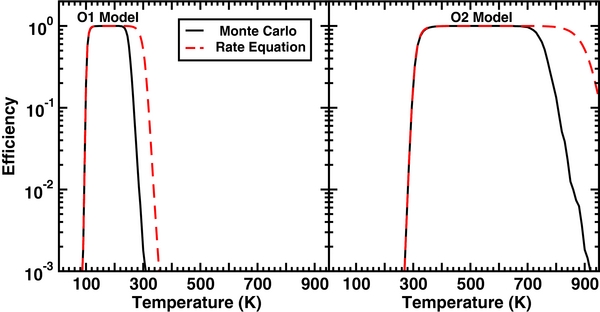
Figure 11. Recombination efficiency as a function of temperature for direct chemisorption models in which 100% of the initially encountered sites involve chemisorption (C sites).
Download figure:
Standard image High-resolution image4.2. Rate of H2 Production
In chemical simulations of interstellar clouds, it is the rate of H2 formation,  , that is the critical process. The rate, which is in units of cm−3 s−1, depends on the calculated effi-ciency η as well as other parameters, as given by the expression

where ng is the grain number density and SH is the sticking coefficient of the H atoms. There are no experimental data regarding the value of the sticking coefficient as a function of temperature, and we therefore use the expression of Hollenbach & McKee (1979):
where Tg and TD are the gas and dust temperatures, respectively, which are here assumed to be the same. Equation (20) can also be written in the simple form

where k is a rate coefficient with units cm3 s−1. Equation (22) is derived using the dust-to-gas number density ratio to convert the grain density to the density of hydrogen nuclei. This ratio is normally taken to be 1.3 × 10⁻¹² for grains with radius 0.1 μm.
To obtain overall rates, we use two values of the atomic hydrogen density—nH = 1 cm−3 and nH = 10 cm−3—and neglect any hydrogen in molecular form. The absolute rates we obtain do not really apply to cold dense clouds, where the surface is covered with ices. Our plots of calculations of R in Figure 12 for Models O1, C1, O3, and C3 as a function of temperature for grains of radius 0.1 μm do show the effect of chemisorption in extending the temperature range of large rates to much higher temperatures as compared with pure physisorption models, especially for Models O3 and C3. These models contain deep chemisorption wells, as can be seen in Table 1, but differ slightly from O2 and C2 in having a slightly wider and shallower physisorption–chemisorption barrier (Cazaux & Tielens 2004). We plot results for both the rate equation approach and our Monte Carlo simulation; as expected from our efficiency calculations, the rates for H2 formation obtained by the former tend to be larger and to extend to higher temperatures.

Figure 12. Rate of H2 production for Models O1, C1, O3, and C3 as a function of grain temperature for different atomic hydrogen densities. The results of both rate equation and Monte Carlo models are shown. The plot is for grains of radius 0.1 μm.
Download figure:
Standard image High-resolution image
For modelers interested in running high-temperature models that include H2 formation on surfaces with deep chemisorption wells, we have provided Table 2, in which Monte Carlo results for H2 recombination efficiencies using Models O3 and C3, which show the largest high-temperature efficiencies, are listed as a function of temperature for two different atomic hydrogen densities: 1 cm−3 and 10 cm−3. To use Table 2, one needs to use the following formula to calculate the H2 formation rate:

Here θ and ϕ are the fractions of silicate and carbonaceous grains, respectively, ηo is the efficiency on silicate grains and ηc is the efficiency on carbonaceous grains and all other factors are the same as in Equation (20). It is to be noted that for Models O3 and C3, the efficiency does not depend on atomic hydrogen number density in the range calculated (0.1–100 cm−3) below 650 K. This effect is similar to what occurs in Model O1, where the efficiency does not depend on hydrogen number density below 200 K, as shown in Figure 7. Thus, although the efficiency values tabulated in Table 2 are for atomic hydrogen number densities of 1 and 10 cm−3, these values can be used for a cloud with any atomic hydrogen number density (including warm dense clouds) in the range calculated provided the dust temperature is below 650 K. A similar story concerns grain size: although grains of radius 0.1 μm were used to determine the efficiencies, there is little dependence of efficiency on granular size below 650 K.
Table 2. Calculated Efficiencies for H2 Recombination as a Function of Temperature for Models O3 and C3
| T (K) | Olivine (Model O3) | Carbon (Model C3) | ||
|---|---|---|---|---|
| ηo | ηc | |||
| nH = 1a | nH = 10 | nH = 1 | nH = 10 | |
| 5 | 1.00(+00) | 9.99(−01) | 9.87(−01) | 9.87(−01) |
| 15 | 1.00(+00) | 1.00(+00) | 9.91(−01) | 9.90(−01) |
| 25 | 6.90(−01) | 6.90(−01) | 7.86(−01) | 7.87(−01) |
| 35 | 4.28(−01) | 4.28(−01) | 5.01(−01) | 5.04(−01) |
| 45 | 3.16(−01) | 3.16(−01) | 5.00(−01) | 4.99(−01) |
| 55 | 2.62(−01) | 2.62(−01) | 4.94(−01) | 4.94(−01) |
| 65 | 2.25(−01) | 2.25(−01) | 4.82(−01) | 4.84(−01) |
| 75 | 1.97(−01) | 1.97(−01) | 4.67(−01) | 4.69(−01) |
| 85 | 1.77(−01) | 1.77(−01) | 4.51(−01) | 4.51(−01) |
| 95 | 1.60(−01) | 1.60(−01) | 4.32(−01) | 4.32(−01) |
| 105 | 1.46(−01) | 1.46(−01) | 4.12(−01) | 4.12(−01) |
| 115 | 1.34(−01) | 1.34(−01) | 3.90(−01) | 3.91(−01) |
| 125 | 1.24(−01) | 1.24(−01) | 3.71(−01) | 3.73(−01) |
| 135 | 1.16(−01) | 1.16(−01) | 3.56(−01) | 3.55(−01) |
| 145 | 1.09(−01) | 1.09(−01) | 3.38(−01) | 3.38(−01) |
| 155 | 1.02(−01) | 1.02(−01) | 3.22(−01) | 3.22(−01) |
| 165 | 9.65(−02) | 9.65(−02) | 3.09(−01) | 3.07(−01) |
| 175 | 9.14(−02) | 9.14(−02) | 2.95(−01) | 2.94(−01) |
| 185 | 8.67(−02) | 8.67(−02) | 2.80(−01) | 2.81(−01) |
| 195 | 8.24(−02) | 8.24(−02) | 2.69(−01) | 2.69(−01) |
| 205 | 7.88(−02) | 7.88(−02) | 2.59(−01) | 2.58(−01) |
| 215 | 7.52(−02) | 7.52(−02) | 2.48(−01) | 2.48(−01) |
| 225 | 7.21(−02) | 7.21(−02) | 2.38(−01) | 2.39(−01) |
| 235 | 6.93(−02) | 6.92(−02) | 2.29(−01) | 2.30(−01) |
| 245 | 6.66(−02) | 6.65(−02) | 2.21(−01) | 2.22(−01) |
| 255 | 6.40(−02) | 6.42(−02) | 2.13(−01) | 2.14(−01) |
| 265 | 6.17(−02) | 6.19(−02) | 2.07(−01) | 2.07(−01) |
| 275 | 5.94(−02) | 5.96(−02) | 2.01(−01) | 2.00(−01) |
| 285 | 5.65(−02) | 5.75(−02) | 1.98(−01) | 1.94(−01) |
| 295 | 5.20(−02) | 5.49(−02) | 2.03(−01) | 1.90(−01) |
| 305 | 4.67(−02) | 5.15(−02) | 2.17(−01) | 1.92(−01) |
| 315 | 4.21(−02) | 4.66(−02) | 2.30(−01) | 2.01(−01) |
| 325 | 3.91(−02) | 4.24(−02) | 2.38(−01) | 2.14(−01) |
| 335 | 3.69(−02) | 3.88(−02) | 2.38(−01) | 2.23(−01) |
| 345 | 3.56(−02) | 3.67(−02) | 2.37(−01) | 2.26(−01) |
| 355 | 3.42(−02) | 3.46(−02) | 2.32(−01) | 2.26(−01) |
| 365 | 3.28(−02) | 3.33(−02) | 2.26(−01) | 2.23(−01) |
| 375 | 3.20(−02) | 3.23(−02) | 2.20(−01) | 2.18(−01) |
| 385 | 3.11(−02) | 3.14(−02) | 2.14(−01) | 2.13(−01) |
| 395 | 3.05(−02) | 3.06(−02) | 2.09(−01) | 2.08(−01) |
| 405 | 2.97(−02) | 2.96(−02) | 2.04(−01) | 2.03(−01) |
| 415 | 2.90(−02) | 2.89(−02) | 1.99(−01) | 1.98(−01) |
| 425 | 2.85(−02) | 2.83(−02) | 1.94(−01) | 1.93(−01) |
| 435 | 2.76(−02) | 2.77(−02) | 1.88(−01) | 1.89(−01) |
| 445 | 2.70(−02) | 2.69(−02) | 1.85(−01) | 1.85(−01) |
| 455 | 2.65(−02) | 2.63(−02) | 1.80(−01) | 1.80(−01) |
| 465 | 2.58(−02) | 2.59(−02) | 1.75(−01) | 1.76(−01) |
| 475 | 2.53(−02) | 2.54(−02) | 1.72(−01) | 1.72(−01) |
| 485 | 2.47(−02) | 2.48(−02) | 1.68(−01) | 1.68(−01) |
| 495 | 2.43(−02) | 2.43(−02) | 1.65(−01) | 1.65(−01) |
| 505 | 2.38(−02) | 2.38(−02) | 1.62(−01) | 1.61(−01) |
| 515 | 2.34(−02) | 2.35(−02) | 1.58(−01) | 1.58(−01) |
| 525 | 2.29(−02) | 2.29(−02) | 1.55(−01) | 1.55(−01) |
| 535 | 2.24(−02) | 2.25(−02) | 1.52(−01) | 1.52(−01) |
| 545 | 2.20(−02) | 2.20(−02) | 1.49(−01) | 1.49(−01) |
| 555 | 2.17(−02) | 2.17(−02) | 1.46(−01) | 1.46(−01) |
| 565 | 2.15(−02) | 2.13(−02) | 1.43(−01) | 1.43(−01) |
| 575 | 2.10(−02) | 2.10(−02) | 1.41(−01) | 1.41(−01) |
| 600 | 2.01(−02) | 2.00(−02) | 1.35(−01) | 1.35(−01) |
| 625 | 1.92(−02) | 1.92(−02) | 1.29(−01) | 1.29(−01) |
| 650 | 1.83(−02) | 1.86(−02) | 1.23(−01) | 1.24(−01) |
| 675 | 3.31(−03) | 1.24(−02) | 1.08(−01) | 1.18(−01) |
| 700 | 9.08(−04) | 5.73(−03) | 8.66(−02) | 1.11(−01) |
| 725 | 2.23(−04) | 1.95(−03) | 4.11(−02) | 9.54(−02) |
| 750 | 4.15(−05) | 4.08(−04) | 1.57(−02) | 6.55(−02) |
| 775 | 1.23(−05) | 1.13(−04) | 4.06(−03) | 3.20(−02) |
| 800 | 2.34(−06) | 2.24(−05) | 1.26(−03) | 1.22(−02) |
| 825 | 7.69(−07) | 1.02(−05) | 4.15(−04) | 4.14(−03) |
5. SUMMARY
With the simple physisorption–chemisorption model of Cazaux & Tielens (2004) and the use of the CTRW Monte Carlo method, we have studied the formation of H2 on the surface of interstellar dust grains of olivine and carbon over a wide dust temperature range from 5 to 825 K. Our major conclusion is that reasonable efficiencies for H2 recombination can occur at temperatures up to ≈700 K if deep chemisorption wells (30,000 K) coexist with weak physisorption sites. Our results are only in fair agreement with those obtained by the rate equation approach at lower temperatures (Cazaux & Tielens 2004, 2010). As the temperature increases, the discrepancy increases strongly. The rate equation method gives a much wider range of temperatures for reasonable production of H2, approaching a high-temperature limit of 1000 K for models with deep chemisorption wells.
Both the Monte Carlo method and the rate equation method show that the temperature range of efficient recombination decreases as the chemisorption wells are made more shallow, and that for pure physisorption the temperature range is miniscule and at very low temperature only for both olivine and carbon, confirming the work of Katz et al. (1999). Using a rough rather than a flat surface enlarges the temperature range somewhat, as in the prior work of Cuppen & Herbst (2007), but the effect of roughness is much smaller than the effect of even relatively weak chemisorption wells.
We investigated the mechanism of H2 formation in some detail, and confirmed the result of Cazaux & Tielens (2004) that tunneling, if it actually occurs, plays a significant role in H2 formation at low temperatures, but with the increase of surface temperature, the thermal mobility of adatoms increases rapidly and thermal hopping of H atoms dominates. We also investigated the dependence of the recombination efficiency over a wide temperature range on the hydrogen atom flux and on grain size. For grains with physisorption and chemisorption sites, we found that the effects were strong only at the highest temperatures, where higher fluxes and larger grain sizes lead to higher efficiencies over larger temperature ranges. Throughout the paper, we have looked at fractional surface coverage as a method of determining in detail what processes are occurring, but coverage can be a misleading indicator if not looked at carefully. For example, low coverage could mean a very high efficiency, in which all H atoms landing on the grain quickly react to form H2, which is immediately ejected. Or low coverage can mean low efficiency, because the atoms desorb quickly rather than react. At higher temperatures, where desorption is rapid, low coverage would tend to correlate with low efficiency, whereas at lower temperatures, where desorption can be slow, low coverage can correlate with high efficiency. Only at high temperatures with rapid desorption is the simple explanation that low coverage leads to a discrepancy between the kinetic Monte Carlo calculations and rate equation calculations correct. The explanation is even more complex with our physisorption–chemisorption models.
We also considered a model based on models O1 and O2 that incorporates direct adsorption into barrierless chemisorption sites and diffusion only into other chemisorption sites. We found a simple temperature dependence in which the H2 formation efficiency is high only at intermediate temperatures. The results obtained with rate equations are similar to those from our kinetic Monte Carlo calculation except at high temperatures, where the efficiency with rate equations is higher because of the low coverage.
For use in chemical simulations of interstellar clouds, we tabulated the efficiency of H2 formation obtained with our Monte Carlo simulations for our standard physisorption–chemisorption model using flat models (O3 and C3), which contain deep chemisorption wells for both olivine and carbon surfaces with features that allow H2 formation at the highest temperatures. Table 2 lists our results over the dust temperature range 5–825 K for two values of the atomic hydrogen density. At temperatures under 650 K, the results are independent of atomic hydrogen density and grain size over the range calculated. The tabulated efficiencies can then be used in the formula for the rate of molecular hydrogen formation, as shown in Equation (23).
K.A. thanks The Ohio State University for a Visiting Scholar position. E.H. acknowledges the support of the National Science Foundation for his astrochemistry program and his program in chemical kinetics through the Center for the Chemistry of the Universe. He also acknowledges support from the NASA Exobiology and the Evolutionary Biology program through a subcontract from the Rensselaer Polytechnic Institute.