


ABSTRACT
In the present work we study the evolution of an active region after the eruption of a coronal mass ejection (CME) using observations from the EIS and XRT instruments on board Hinode. The field of view includes a post-eruption arcade, a current sheet, and a coronal dimming. The goal of this paper is to provide a comprehensive set of measurements for all these aspects of the CME phenomenon made on the same CME event. The main physical properties of the plasma along the line of sight—electron density, thermal structure, plasma composition, size, and, when possible, mass—are measured and monitored with time for the first three hours following the CME event of 2008 April 9. We find that the loop arcade observed by EIS and XRT may not be related to the post-eruption arcade. Post-CME plasma is hotter than the surrounding corona, but its temperature never exceeds 3 MK. Both the electron density and thermal structure do not show significant evolution with time, while we found that the size of the loop arcade in the Hinode plane of the sky decreased with time. The plasma composition is the same in the current sheet, in the loop arcade, and in the ambient plasma, so all these plasmas are likely of coronal origin. No significant plasma flows were detected.
Export citation and abstract BibTeX RIS
1. INTRODUCTION
Coronal mass ejections (CMEs) are the most spectacular and energetic events in the solar system and consist of a sudden acceleration of large amounts of plasma in the solar atmosphere and their release in the heliosphere. Despite the large body of observations and theoretical work devoted to CMEs, we are still far from a consensus on how the corona is able to generate, accelerate, and heat CME plasmas. CMEs are complex events: they are not limited to the ejection of material into space, but also involve the development of a current sheet (CS) behind the CME ejecta and the formation of a post-eruption loop arcade, as well as the sudden dimming of coronal radiation around the ejection site. While a large number of studies have been devoted to one or a few of the many aspects of a CME, one of the main obstacles to advances in CME science is the lack of comprehensive quantitative descriptions of all plasmas involved in the same CME event.
Recently, Landi et al. (2010) observed the initial acceleration phases of the CME ejecta of 2008 April 9 with an array of space instruments on board Hinode, SOHO, and STEREO. They measured the physical properties and heating rate of the core of the CME ejecta and determined the electron density, the thermal structure, and the dynamic evolution of the core as a function of time; they also compared them to theoretical models of CME initiation and propagation. Their study was limited to analyzing the physical properties of the core of the CME ejecta. However, their data set included the signatures of all other features in a CME: post-eruption arcade (PEA), CS, and coronal dimming (CD). These phenomena are very important as they are the signatures of the re-organization of the host active region after the large-scale loss of equilibrium during the CME eruption; also, the CS evolution bears the signatures of the ongoing magnetic reconnection process.
The aim of this paper is to use EIS and XRT observations to quantitatively determine the physical properties of the plasma in the PEA, CS, and CD; these measurements are made as a function of time. This work extends the study of Landi et al. (2010) to the plasma left behind by the CME ejecta, and also complements the results obtained by Savage et al. (2010) and Patsourakos & Vourlidas (2011) on the CS of the same CME event studied here. A future paper (E. Landi et al. 2012, in preparation) will be devoted to the determination of the thermal structure of the hot plasma that Landi et al. (2010) reported to be following the CME core, as well as the predicted charge state signatures of the 2008 April 9 CME in in situ observations. Together, these works aim at providing a complete quantitative description of all aspects of a single CME event that will hopefully be helpful in constraining theoretical models of CME heating and acceleration.
A very brief overview of the current knowledge about PEA, CS, and CD plasmas is given in Section 2. The observations and the selection of the regions we analyzed are described in Section 3, where the diagnostic techniques we used are also introduced. In Section 4 we describe the results and in Section 5 we compare them to earlier measurements. This work is summarized in Section 6.
2. POST-CME PLASMA EVOLUTION
In this subsection we provide a brief description of the current knowledge about the plasma evolution in the host active region after the CME ejecta have left the Sun. This overview is by no means exhaustive and is only provided as context for our work.
2.1. Post-eruption Arcades
PEAs have been commonly observed after nearly all CME eruptions (Schwenn et al. 2006). For example, Tripathi et al. (2004) report that a one-to-one relationship existed between PEAs and CMEs in 236 events observed between 1997–2002 and they even suggest that PEAs can be used as tracers of CME events even when the observations were not made in time to capture the ejecta acceleration. PEAs normally last between 2 and 20 hr (Tripathi et al. 2004), and their physical properties have been summarized by Fletcher et al. (2011): PEA plasma is characterized by multimillion-degree temperature with high pressure and density, which cools slowly with time and drains material down toward lower heights.
PEAs are a normal expectation from theory (McKenzie & Hudson 1999) and are due to large-scale magnetic restructuring after the CME ejection as a consequence of magnetic reconnection and plasma inflows that fill magnetic loops at large heights with hot material coming from the reconnection site that has evaporated from the chromosphere. Hotter loops are expected to be formed at the top of the arcade, close to the reconnection site; then they cool and move down in the arcade because of the influx of new material from the reconnection site that is forming new hot loops at larger heights (Lin et al. 2004). The temperature and density reached by PEAs are related to the rate of energy release in the reconnection site above the arcade. The measurement of these quantities as a function of time can thus help to constrain the rate of reconnection in theoretical models and its evolution with time.
2.2. Coronal Dimmings
CDs consist of a sudden drop in the intensity of a region in the corona after the CME has been ejected, and can extend in height from 1.1 R☉ up to 2.5 R☉ (Howard & Harrison 2004). They are observed by both spectrometers and imaging instruments at the solar limb as regions darker than the coronal background, and they are coronal manifestations of transient coronal holes appearing on the disk after CME events (Miklenic et al. 2011). CDs are commonly observed in lines emitted by ions formed at around 1 MK (Harrison & Lyons 2000; Harra et al. 2007; Robbrecht & Wang 2010), but sometimes they are seen at all temperatures (Harra et al. 2007). Not all CMEs have been reported to be followed by dimmings (Reinard & Biesecker 2008, 2009), and CMEs with dimmings were found to be on average faster than those without ones (Reinard & Biesecker 2009).
CDs occur suddenly, but the recovery of the lost intensity is a much slower process (Reinard & Biesecker 2008). The time of their appearance has been shown to be tied to the time of CME acceleration and energy release in a flare (Miklenic et al. 2011), although sometimes dimmings start before the CMEs and peak after the CME has left the region (Howard & Harrison 2004). The disappearance of transient coronal holes on the disk was found to be due to the shrinking of the hole region rather than the heating of local plasma (Kahler & Hudson 2001), and Attrill et al. (2008) suggested that such recovery is due to the reconnection of open field lines to closed magnetic loops, as suggested by Fisk & Schwadron (2001) for the quiet corona. However, the transition region plasma was also suggested as a source for replenishing the dimmed region (Imada et al. 2007; Jin et al. 2009), and outflows in transition region lines within CDs were indeed observed (Harra & Sterling 2001).
There are several processes that can generate a dimming: a density decrease and mass loss (due to outflows) or temperature variations that decrease the fractional abundance of the ions formed at around 1 MK emitting the lines whose intensity decreases in CDs (Attrill et al. 2006 and references therein; Howard & Harrison 2004). Plasma outflows associated with dimmings and transient coronal holes have been reported in many occasions (Harra & Sterling 2001; Harra et al. 2007; Jin et al. 2009; Miklenic et al. 2011) and suggest that part or most of the CME mass can actually be provided by the plasma lost during the dimming event. In fact, the mass lost in CDs was found to be smaller than, but comparable to, the total CME mass (Harrison et al. 2003; Howard & Harrison 2004; Reinard & Biesecker 2008; Jin et al. 2009).
As a consequence, CDs are important in the overall CME event as signatures of the source regions of the bulk CME material, as well as a tracer of the effects of CME acceleration and of CME-related shocks on the local plasma thermal status.
2.3. Current Sheets
Post-CME CSs have been observed and studied in a number of occasions. Detailed measurements of the temperature, density, and composition of CS plasma (Ciaravella et al. 2002; Raymond et al. 2003; Ko et al. 2003; Lee et al. 2006; Bemporad et al. 2006; Ciaravella & Raymond 2008; Schettino et al. 2010) have been carried out mostly using spectral observations from the SOHO/UVCS instrument (Kohl et al. 1995), although a few density determinations have been done using SUMER spectra (Innes et al. 2003; Wang et al. 2007) and white light data (e.g., Webb et al. 2003; Patsourakos & Vourlidas 2011), which also provided evidence of plasma flows.
A combination of white light and UVCS observations with modeling has allowed the determination of the geometry and size of the CS. In general, CS plasma was found to be denser than the surrounding ambient plasma, and very hot, with temperatures ranging from around 3–4 MK (Bemporad et al. 2006) up to 10 MK (Schettino et al. 2010; Bemporad et al. 2006) or 20 MK (Innes et al. 2003); the electron temperature was found to slowly decrease with time in the few studies that monitored CS evolution (Bemporad et al. 2006; Ciaravella & Raymond 2008; Schettino et al. 2010). The electron density was found to be either constant (Bemporad et al. 2006) or slowly decreasing (Ciaravella & Raymond 2008). Measurement of the plasma composition revealed the presence of the abundance anomalies known as the first ionization potential (FIP) effect, consisting of an enhancement of the abundance of elements with FIP smaller than 10 eV from photospheric values (low-FIP elements), while the abundance of elements with FIP > 10 eV (high-FIP elements) are unchanged (e.g., Feldman & Laming 2000). The factor of a low-FIP enhancement (the "FIP bias") was, however, different in a different CS, ranging from typical coronal values of ≈3 (Ko et al. 2003) to 4–5 (Bemporad et al. 2006) and even 7–8 (Ciaravella et al. 2002).
The formation and physical properties of post-CME CSs are very important, as they are predicted to form in almost all CME models and to connect the PEA in the CME acceleration site with the CME ejected core (e.g., Vrsnak et al. 2009, and references therein). CSs are a key ingredient in both the analytical and numerical simulation of CMEs.
2.4. Earlier Results from a 2008 April 9 CME Event
The 2008 April 9 event observed by Hinode, STEREO, and SOHO provides us a unique opportunity for two reasons. First, it allows us to carry out detailed measurements of the properties of PEA, CD, and CS plasmas and of the relationship between CS and PEA plasmas at much lower heights than previously (≈1.1 R☉). Second, it allows us to exploit the combination of the full range of spectral lines observed by Hinode/EIS with the X-ray data from Hinode/XRT to investigate the whole range of temperatures from 0.6 MK to more than 10 MK. For comparison, earlier UVCS studies were carried out at heights larger than 1.4 R☉ and used lines from Ca xiv, Fe xviii and, in a few instances, Si xii and Fe xv.
The CS plasma of this event was previously studied by Savage et al. (2010) and Patsourakos & Vourlidas (2011). The latter used STEREO/SECCHI and SOHO/LASCO coronographic observations to determine the morphology, density, and temperature of this structure and demonstrated that it was indeed the CS predicted by theoretical models to form after the CME was ejected; they further determined that it was denser and hotter than the surrounding corona and significantly displaced from the post-CME loops in the active region that hosted the event. Savage et al. (2010) analyzed the XRT and LASCO observations focusing both on the CS and the PEA. They found that the CS harbors downflows and upflows, while upflows and disconnection events occur at the top of the PEA. From the pattern of upflows and downflows shown in Figure 13 of Savage et al. (2010), it appears that the CS X-line rose from 0.13 to 0.29 R☉ above the limb during the time of the observations; however, EIS observations pertain to plasma observed at ≈0.1 R☉ from the limb. Thus, our observations may be more closely related to the Innes et al. (2003) observations of the downflow region above the flare loops and Atmospheric Imaging Assembly observations of very hot supra-arcade plasma (Reeves & Golub 2011) than to the UVCS observations at larger heights.
These studies highlighted the presence of CS and PEA plasmas; however, Patsourakos & Vourlidas (2011) measured the physical properties at heights above 2 R☉, while Savage et al. (2010), concentrating on XRT and LASCO images only, could not provide the detailed measurements of the plasma physical properties close to the Sun that are the focus of the present work.
3. OBSERVATIONS
The CME we observed was activated at around 9:10 UT on 2008 April 9 during the Whole Heliosphere Interval coordinated campaign. It consisted of the standard three components: a fast front, a cavity, and a core that hosted an erupting prominence. The event was observed by an array of instruments from two different directions: the Earth–Sun direction and the STEREO-A–Sun direction. We restrict our analysis to the observations from EIS and XRT on board Hinode as these are the two instruments that provide the diagnostic tools we need for the present study. EIS allows detailed high-resolution spectroscopic diagnostics to be carried out on the emitting plasmas, while XRT provided X-ray observations of the event and thus sampled the plasma's hottest component.
3.1. EIS Observations
EIS observations were made on 2008 April 9, between 06:20 UT and 17:32 UT. EIS carried out a series of sit-and-stare deep exposures taken with a 10 minute cadence, and the entire wavelength range was transmitted to the ground. The field of view (FOV) of 2'' × 512'', centered at (1000'', −412''), is shown in Figure 1, superimposed on a sequence of Hinode/XRT images. A description of the EIS instrument can be found in Culhane et al. (2007). The direction of the EIS line of sight relative to a schematic of the CME source region and trajectory are shown in Figure 2, adapted from Forbes & Acton (1996).

Figure 1. Time series of XRT Al-poly images of the SW quadrant after the CME event. The EIS slit field of view is superimposed as a white line. The southern edge of the EIS slit stretches beyond the XRT field of view, down to Y = −670''.
Download figure:
Standard image High-resolution image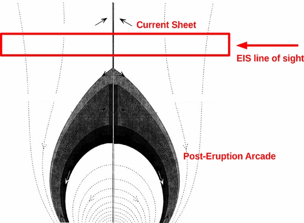
Figure 2. Schematic showing the portion of the post-eruption arcade and current sheet imaged by EIS (adapted from Forbes & Acton 1996). The region observed by EIS is included in the red rectangle. Even if EIS was observing in sit-and-stare mode, the field of view relative to the XEA cusp is wide because the XEA shrinks with time and decreases its height. EIS observes plasma at progressively larger heights in the schematic.
Download figure:
Standard image High-resolution imageEIS observations were carried out continuously, but problems in the telemetry caused the data to be lost, and part of them was recovered in non-standard format. Data reduction, cleaning, and calibration were done with an ad hoc procedure, which is fully described in Landi et al. (2010). The data were recovered for almost all data sets in the 06:20 UT to 13:55 UT time interval, but from time to time data gaps made a few subsections of the EIS wavelength intervals unavailable. After 13:35 UT the available data decreased until none were available after 13:55 UT.
3.2. XRT Observations
During the EIS observations, XRT was carrying out a sequence that imaged the SW quadrant of the Sun, centered at X = 833'', Y = −384''. Frames were taken with a one-minute cadence and included a 512'' × 512'' FOV. Only the Al-poly filter was used, so XRT data cannot be used for plasma diagnostic purposes with filter ratios. The Al-poly filter is optimized to observe wavelengths below 50 Å, but its effective area has a long-wavelength tail between 170 Å and 190 Å where the sensitivity is non-negligible, which partially overlaps the EIS short-wavelength channel. Data were reduced and calibrated using the latest effective areas (Narukage et al. 2011). This new calibration significantly changes the effective area of the Al-poly filter over the previous one, and decreases it significantly above 170 Å so that the contribution of the EIS short-wavelength range to the total count rate observed by XRT is smaller than previously assumed.
3.3. Region Selection
Figure 1 shows a series of XRT images that illustrates the evolution of the active region after the CME onset, including the formation of a CS. The EIS slit is superimposed onto each panel and the X-ray feature crosses it in the middle. By using a 2'' slit in a sit-and-stare mode, EIS cannot provide images like XRT. However, by placing side-by-side images of the EIS slit in a given spectral line obtained from a series of consecutive exposures, we can build time-intensity images such as the one shown in Figure 3. In this figure, the Y-axis represents the coordinate along the EIS slit (along the solar N–S direction), while the X-axis represents time, from before the CME event to a few hours afterward. Each position along the X-axis represents a single EIS exposure. We have shown lines from six ions as proxies of six different temperature regimes: He ii (log Tmax = 4.7) for the lower transition region; Fe viii (log Tmax = 5.6) for the upper transition region; Fe xii (log Tmax = 6.2) for the quiet corona, Fe xiii (log Tmax = 6.25) and Fe xv (log Tmax = 6.35) for the active corona, and Fe xvi (log Tmax = 6.45) for the very active corona. Figure 3 summarizes the entire event. Between 9:40 UT and 10:20 UT a CME crosses the EIS FOV, and its core is observed as an intense emission feature in the ions formed below 106 K (He ii and Fe viii) and as a decrease of emission in ions formed at typical coronal temperatures (Fe xii). After the CME event, hot plasma fills the region of the slit where the CME has passed and is most prominent in the Fe xiii to Fe xvi line emission. Landi et al. (2010) showed that no emission was present in the Fe xvii λ204.7 line, indicating that plasma at subflare temperatures was not present. In the lower part of the slit, coronal emission decreases substantially and forms a CD.
In order to determine whether the EIS hot feature corresponds to the bright plasma in the XRT images and to combine the two instruments for diagnostic purposes, it is necessary to extract from the XRT data set the subset of data that corresponds to the EIS data set. Time-intensity images from XRT directly comparable to those shown in Figure 3 can be built by carving the FOV of the EIS slit from each of the consecutive XRT images and lining them in a new two-dimensional image where the Y-axis corresponds to a position along the EIS slit, and the X-axis is time. The resulting XRT image, with the contours of the EIS He ii and Fe xv line intensities superimposed, is shown in Figure 4, where the XRT data have been rebinned in time to match exactly the EIS cadence. Figure 4 shows that the X-ray emission from the brighter feature is approximately cospatial to the Fe xv emission after the CME event. Both features experience the same evolution in time, by shrinking constantly. The similarity in shape and evolution suggests that XRT and EIS are observing the same feature.
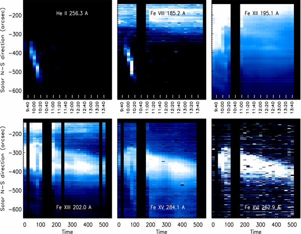
Figure 3. EIS time-intensity images using the intensities of lines from the following ions: He ii (log Tmax = 4.7), Fe viii (log Tmax = 5.6), Fe xii (log Tmax = 6.2), Fe xiii (log Tmax = 6.25), Fe xv (log Tmax = 6.35), and Fe xvi (log Tmax = 6.45).
Download figure:
Standard image High-resolution image
Figure 4. Top: XRT time-intensity images of the EIS slit field of view, rebinned to match EIS time resolution. Contours of the He ii (blue) and Fe xv (red) line emission are superimposed on the image to mark the passage of the CME core (He ii) and the presence of the current sheet (Fe xv). Bottom: normalized, background subtracted intensity profile along the EIS slit field of view of the Al-poly filter emission (black) and of the EIS Fe xv λ284.1 line (red), taken at 11:00 UT (left) and 13:20 UT (right).
Download figure:
Standard image High-resolution imageFigure 5 displays the time-intensity images of the Fe xii λ195.1 and Fe xv λ284.1 lines and the XRT Al-poly filter. The areas we chose for the analysis are also shown and they have been selected as follows: above the bright feature, corresponding to the upper 84 pixels of the EIS slit ("A" data set); below the bright feature, corresponding to the lowest 100 pixels of the EIS slit ("B" data set); and along the bright feature, selected using the Fe xv line intensity ("BF" data set). For each time bin, the spectra from all the pixels within each of the three selected regions were averaged so that the physical properties of each of them could be measured as a function of time. The lines that have been used in the analysis are listed in Table 1, along with the temperature of the maximum abundance of the emitting ion. The list of ions available in Table 1 is different from that provided by Landi et al. (2010). The reason for this is that the plasmas that we are studying are very different: Landi et al. (2010) studied the properties of the CME core plasma, while here we are interested in the larger, longer-lasting plasma structures in the entire EIS slit. None of the lines emitted by the chromospheric and transition region plasmas reported by Landi et al. (2010), such as He ii, O iv, v, Mg v, Al viii, and Si vi, were detected in the present data sets because they were only emitted by the CME core; on the contrary, lines from other ions formed at high temperatures unavailable to Landi et al. (2010), like S xi, xii, xiii, Ca xiv, Fe xvi, and Ni xvii, could be measured.
Table 1. Lines Used in the Present Work
| Ion | Wvl. | log Tmax | Ion | Wvl. | log Tmax |
|---|---|---|---|---|---|
| (Å) | (Å) | ||||
| Mg vi | 268.991 | 5.63 | Fe viii | 185.213 | 5.62 |
| Mg vii | 276.154 | 5.78 | Fe viii | 186.599 | 5.62 |
| Mg vii | 280.742 | 5.78 | Fe viii | 194.661 | 5.62 |
| Al viii | 250.139 | 5.92 | Fe viii | 195.972 | 5.62 |
| Al ix | 280.135 | 6.03 | Fe ix | 197.862 | 5.87 |
| Al ix | 282.421 | 6.03 | Fe x | 174.531 | 6.04 |
| Al ix | 286.376 | 6.03 | Fe x | 175.263 | 6.04 |
| Si vii | 272.648 | 5.78 | Fe x | 177.240 | 6.04 |
| Si vii | 275.361 | 5.78 | Fe xi | 182.169 | 6.13 |
| Si vii | 275.676 | 5.78 | Fe xi | 188.232 | 6.13 |
| Si ix | 290.687 | 6.05 | Fe xi | 192.830 | 6.13 |
| Si x | 253.788 | 6.15 | Fe xii | 186.887 | 6.19 |
| Si x | 258.371 | 6.15 | Fe xii | 192.394 | 6.19 |
| Si x | 261.044 | 6.15 | Fe xii | 195.119 | 6.19 |
| Si x | 272.006 | 6.15 | Fe xiii | 201.128 | 6.25 |
| S x | 257.147 | 6.18 | Fe xiii | 202.044 | 6.25 |
| S x | 259.497 | 6.18 | Fe xiii | 203.828 | 6.25 |
| S x | 264.231 | 6.18 | Fe xiv | 211.318 | 6.29 |
| S xi | 246.895 | 6.28 | Fe xiv | 264.790 | 6.29 |
| S xi | 247.159 | 6.28 | Fe xiv | 270.522 | 6.29 |
| S xi | 281.402 | 6.28 | Fe xiv | 274.204 | 6.29 |
| S xi | 285.588 | 6.28 | Fe xv | 284.163 | 6.34 |
| S xii | 288.421 | 6.35 | Fe xvi | 262.976 | 6.43 |
| S xiii | 256.685 | 6.42 | Ni xvii | 249.178 | 6.49 |
| Ca xiv | 193.866 | 6.57 |
Note. Wavelengths are from V.6.0.1 of CHIANTI; wavelengths of lines made of self-blends are taken from the strongest transition in the spectral feature.
Download table as: ASCIITypeset image
In the BF data set, we carried out part of the analysis by both removing the background ambient emission, and not removing it. Background emission was determined for each line in each exposure with a linear or quadratic fit to the line intensity outside the bright region; the amount of pixels included was optimized for each case in order to minimize the effects of noise on the background estimation. Only lines from Fe xiii to Fe xvi, S xiii, and Ni xvii were left with a significant subtracted signal.
3.4. Diagnostic Methods
We measured the plasma is physical properties applying standard diagnostic techniques to EIS spectral line intensities. We measured the electron density using line intensity ratios, while we determined the differential emission measure (DEM) of the plasma using the iterative technique developed by Landi & Landini (1997). Since the available XRT data consist of images in one filter only, no diagnostics can be carried out using XRT alone and thus we use the EIS-derived DEM to predict the XRT Al-poly spectrum in the 1–200 Å range. The resulting spectrum is folded through the XRT Al-poly effective area to calculate the predicted count rates. These are compared to observations to understand whether additional hot components are present in the FOV, which cannot be detected with EIS alone.
In our analysis we used Version 6.0.1 of the CHIANTI database (Dere et al. 1997, 2009) and calculated the line emissivities adopting the ion fractions of Bryans et al. (2009) and the coronal abundances from Feldman et al. (1992). Since the FIP of the ions emitting almost all EIS lines is lower than 10 eV, the choice of the element abundance data set affects only the absolute value of the DEM, but not its temperature dependence. Abundance related changes in the overall count rates predicted using the Al-poly filter are more complex and depend on temperature, since different species dominate the Al-poly range at different temperatures. At quiet-Sun coronal temperatures, the H-like and He-like species of C, N, and O dominate the spectrum and their emissivities are not affected by the FIP effect; between log T = 6.2–7.5 Fe lines dominate the spectrum so that the XRT Al-poly response changes almost linearly with the FIP effect. Thus, a direct comparison between EIS and XRT is most vulnerable to errors in the adopted abundances. We will use S x-xiii to investigate the FIP effect in the emitting plasmas.
4. RESULTS
4.1. Region Morphology and Evolution
Figure 1 displays a series of XRT images with a 20 minute cadence that monitors the evolution of the hot plasma crossing the EIS slit from immediately after the CME left the EIS FOV to the end of the available EIS observations. The active region undergoes a significant evolution, from being formed by an unresolved large region brighter than the surrounding areas to forming the CS studied by Patsourakos & Vourlidas (2011) and Savage et al. (2010).
In the top row of Figure 1 the XRT emitting plasma resembles an active region loop arcade extending beyond the EIS slit, whose intensity quickly decreases with distance from the limb. We will refer to this as X-ray emitting arcade (XEA). The size of the XEA shrinks with time and eventually forms a cusp-like structure below the EIS FOV. The elongated shape of the CS can be clearly seen after 13:00 UT in the XRT images as crossing the middle of the EIS slit. Before 13:00 UT, the CS cannot be unambiguously detected in the XRT images. There is a southward-moving, elongated structure observed between 10:26 UT and 11:40 UT crossing the top half of the EIS slit first at ≈300'' (10:26 UT, corresponding to a height above the limb of 1.08 R☉) and then at ≈380'' (11:40 UT, corresponding to a height above the limb of 1.11 R☉). However, such a structure could also be the northern leg of a loop arcade that is progressively shrinking.
Since the XRT plasma crossing the EIS slit experiences such a marked evolution, the question arises as to whether the bright structure observed in Fe xiii-xvi by EIS and corresponding to the BF data set is the CS or not. After 13:00 UT the CS is visible in the XRT images. Before that time, the CS may be embedded in the brighter emission of the XRT arcade but since the latter is dominating the XRT image, the BF data set is likely to be made largely of XEA plasma before 13:00 UT.
In the present work, we measure the physical properties of the plasma in the BF data set at all times. The results will be interpreted as the physical properties of the XEA plasma before 13:00 UT and of the CS after that time. However, some contribution of the background XEA plasma might still be present after 13:00 UT, which cannot be easily subtracted from the BF data set.
Figure 3 shows that the Fe xii intensity decreases significantly in the BF and B data sets. While the decrease in the BF data set could be ascribed to the appearance of the XEA, the decrease in region B is due to the CD following the CME ejecta. It is interesting to note that such a dimming corresponds to a brightening in the Fe xv line emission, indicating that the temperature of the dimmed plasma has increased.
4.2. Size
Figure 5 shows that the X-ray signature of the BF is moving southward and slowly shrinking with time. In order to study the evolution of the BF size, we considered the XRT time sequence and the evolution of the intensity profile along the slit of the brightest line that shows the BF: Fe xv λ284.1. For each spectrum, we first measured the Fe xv and XRT intensities along the EIS slit FOV and then subtracted the background emission. An example of subtracted (and normalized) intensities are given in the bottom panels of Figure 4.
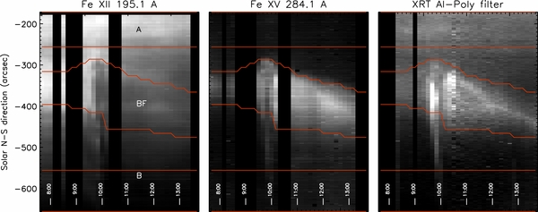
Figure 5. EIS time-intensity maps for Fe xii λ195.1, Fe xv λ284.1, and the XRT Al-poly filter. The regions selected for analysis ("A," north of the bright feature; "B," south of the bright feature; and "BF," inside the bright feature) are also marked.
Download figure:
Standard image High-resolution imageWe found that the two subtracted intensity profiles are similar and the apparent difference in the BF width in Figure 5 is due to a combination of the effect of a different background and of the color scale. The BF is slightly wider in Fe xv than in XRT by ≃10''–20'', comparable to the uncertainty of determining the boundaries of the BF in the background noise at each side. The BF width (i.e., its length along the EIS slit), measured at the base of the feature in the intensity profile, decreases slowly with time, from around 180'' at 10:52 UT to around 130'' at 13:45 UT as determined with XRT, the rate of decrease being a bit faster toward the end of the observations. The time evolution of the width of the BF is shown in the bottom panel of Figure 6, in units of solar radii.

Figure 6. Current sheet mass (top panel) and width measured at the base of the BF intensity profile along the EIS slit direction (bottom panel) evolution as a function of time. The mass has been calculated assuming a cylindrical current sheet (stars) and the slab geometry found by Patsourakos & Vourlidas (2011; triangles).
Download figure:
Standard image High-resolution image4.3. Dynamics
4.3.1. Doppler Shifts
The CS orientation was found to follow rather closely the CME trajectory (Patsourakos & Vourlidas 2011), which was found to lie between the Hinode and STEREO planes of the sky, that is between 0° and ≃24° away beyond the Hinode plane of the sky. This means that flows along the CS and the arcade loops will be difficult to detect with EIS as Doppler shifts unless their speed is faster than 10 km s−1. We used the Fe xii λ195.11 and Fe xv λ284.16 lines to study the presence of flows. The profiles of these lines were fit with a Gaussian shape for each spectrum of the A, B, and BF data sets so that the line centroid, peak intensity, and width could be measured.
The Fe xii line, emitted by the background, was assumed to be at rest and was used to determine the corrections for orbital and slit-dependent variations of the line centroid; the corrections were applied to the Fe xv line centroids and were found to be consistent with the corrections provided by the standard EIS software (Young 2010). Results show that (1) no variation in the Fe xv line centroid was observed in the BF during the entire EIS observation and (2) no difference was found at any time between the Fe xv line centroid in the BF and the values obtained in the A and B data sets. Since the latter two locations correspond to the background plasma, we conclude that no significant Doppler velocity is observed in the BF. We also checked whether asymmetries in line profiles were present that could be the signature of flows in the CS. The only line emitted by the BF bright enough to allow detection of such asymmetries is the Fe xv λ284.163 line, but no trace of them was found in its profile, even though a weaker blending Al ix line at 284.025 Å could be partially masking blueshifts.
4.3.2. Line Widths
The instrumental line FWHM determined by Hara et al. (2011) was subtracted from the measured values. Hara et al. (2011) determined the EIS instrumental width for the 1'' slit by comparing Fe xiv spectral line widths measured from EIS in the EUV and from the Norikura Solar Observatory in the visible λ5303 green line on the same target. Hara et al. (2011) were able to determine both the absolute value of the EIS instrumental line width, as well as the variation in its position along the EIS slit. Since the 2'' slit was used in the present observations, we increased the Hara et al. (2011) instrumental width by 7mÅ, as suggested by Young (2011).
For each of the three data sets we selected, the spectrum was averaged over a relatively wide portion of the EIS slit (see Figure 5), along which the instrumental width varies significantly. For each data set, we adopted the instrumental width averaged over the selected region, and the total variation across the region was used as the uncertainty for the adopted instrumental width. This additional uncertainty was combined with the uncertainty of the measured line width.
The corrected line widths allowed us to determine the temperature Tk, which we define as the temperature of the corrected width assuming zero non-thermal motions. We measured Tk for Fe xii and Fe xv at all times and positions. Results are shown in Figure 7, where diamonds and stars indicate Fe xii and Fe xv results, respectively.

Figure 7. Temperatures Tk for Fe xv (stars) and Fe xii (diamonds). Tk is defined as the ion temperature that can be determined from the line width assuming zero non-thermal motions. The CME ejecta crossed the EIS slit field of view between 9:40 UT and 10:10 UT.
Download figure:
Standard image High-resolution imageData set A shows no evolution in the Tk values obtained at all times, with it being consistently outside the CME ejection site. The Fe xv Tk values are lower than the Fe xii ones at all times, although the differences are almost as large as the uncertainties themselves. In the BF and B data sets, the passage of the CME ejecta corresponds to a large increase in the Tk values of both lines. This increase could be due to four possible effects (or a combination of them): a line of sight averaging of the Doppler shifts caused by the front and back of the expanding CME outer shell; the same type of averaging for the emission of the expanding interior volume of the CME; the thermal width of the shocked ions; or a sudden increase in the non-thermal velocities themselves.
After the CME ejecta leave the EIS slit FOV, data sets B and BF show a different behavior. Data set BF, corresponding to the XEA and CS plasmas, provides Tk values very close to the pre-CME levels, although Fe xii values are somewhat lower than before, while Fe xv values are slightly larger. Data set B, on the other hand, maintains larger values of Tk for both lines, which slowly decrease toward pre-CME levels. The larger values in the Tk provided by Fe xii are likely caused by the plasma belonging to streamers in the foreground and background, which have been displaced by the CME shock during the eruption and are slowly moving back to their original positions. The Fe xv values on the other hand may indicate that the shock associated with the CME eruption has increased the turbulent velocities in the CD region.
In the background, the widths of Si vii, Si x, Fe viii, and Fe ix suggest turbulent speeds of about 40 km s−1. There are few lines from the BF to measure line widths, but if we assume that the ions are formed at their peak temperatures in an ionization equilibrium, the Fe xii and Fe xv line widths indicate turbulent speeds of 58 and 40 km s−1, respectively. Those values are similar to the turbulent line widths in CS measured from the Fe xviii line in the first few hours after flares by Bemporad (2008).
It is interesting to note that different ions provide different Tk values in the background plasma. For example, Fe x,xi provide values in agreement with Fe xii, while Si vii,x provide lower values (3.5–4.5 MK) and Fe viii,ix reach 9–11 MK. This ion-dependent variability of the kinetic temperature might explain in part why our values are much larger than those obtained by Bemporad et al. (2006), as they measured the kinetic temperature using the H i Lyβ line profile.
4.4. Electron Density
To measure the electron density we used the Fe xiii 203.8/202.0 line intensity ratio. The advantage of this ratio over other available ones (from Fe xii, Si x, Fe xiv) is the brightness of the two lines, their stronger sensitivity to the electron density, and the higher accuracy of the atomic data. Also, Fe xiii line emission was observed both in the background and in the BF, while Si x and Fe xii were emitted almost only in the background. However, at densities below 109 cm−3 photoexcitation from background photospheric radiation becomes effective as a populating mechanism for the levels in the ground term of Fe xiii, so that this process has been taken into account when we used CHIANTI to determine the theoretical intensity ratio.
We monitored the evolution of the electron density with time in all three regions. In the BF data set, we used the results of the background subtraction (as described in Section 2.3) to determine the electron density from both the BF and the background. Results are summarized in Figure 8. The plasma in data set A is not affected by the CME event and consistently its electron density is unchanged. Note that even if the plasma belongs to the southern edge of an active region, the density is fairly low (2–3 × 108 cm−3). The background emission at the BF location has a constant density (within uncertainties). On the contrary, the BF plasma density is lower by a factor of ≃ 2 than the background, and thus is apparently more tenuous than the background plasma that surrounds it. The plasma density in data set B slightly increases from the pre-CME values, but uncertainties prevent us from any definitive conclusion since they are larger than the difference in density. It is interesting to note that during the CME event (occurring between the two vertical lines in Figure 8 that mark its start and end times) the plasma density seems to be unaffected.
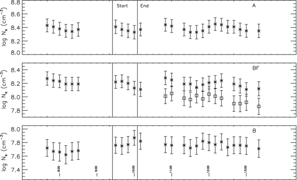
Figure 8. Density diagnostic results for the current sheet for the three selected regions as a function of time. Stars: background density; squares: density of the XEA and CS combined plasmas.
Download figure:
Standard image High-resolution image4.5. Thermal Structure
4.5.1. Differential Emission Measure
Figure 9 shows the DEM curves for each of the three regions. We chose to use the unsubtracted spectrum to determine the BF DEM, because background subtraction left only a very few ions with lines having a sufficient signal to be used for DEM analysis. For each of the regions, the DEM was determined for each of the spectra obtained during the entire EIS observation, so that its evolution with time could be monitored.
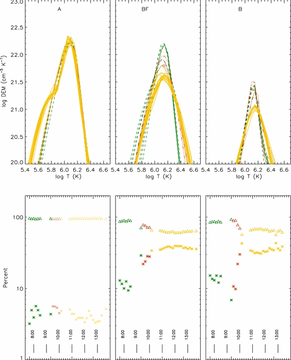
Figure 9. Top: DEM curves for all the selected regions. Bottom: percent contribution of the plasma hotter (triangles) and colder (stars) than log T = 6.2 to the total plasma EM, as a function of time. Green curves: before the CME event. Red curves: during the CME event. Yellow curves: after the CME event.
Download figure:
Standard image High-resolution imageFor each selected region, three colors have been used in Figure 9: green for times before the CME event, red during it, and yellow after the CME left the EIS FOV. The top panels show the DEM curve of the plasmas. In all cases, the DEM is strongly peaked at temperatures in the log T = 6.1–6.2 (T = 1.2–1.6 MK) at all times. This temperature is more typical for quiet Sun than active regions, while, at least before the CME event, there is little material at temperatures higher than 2 MK. The DEM peak value is smaller in the B data set, consistent with its larger distance from the limb.
The plasma in data set A is stable at all times, except for the rise of a low-temperature shoulder below 0.6 MK. Since this happens some time after the CME left the EIS FOV, it is likely that these two events are not related. Even if the plasma sits on top of an active region, it is concentrated into a narrow range around a typical quiet-Sun temperature: log T ≃ 6.1. The BF data set experiences a factor three drop of the DEM peak value at log T = 6.1, showing that a large portion of the ambient corona has either been blown away by the CME or has been heated. This drop may constitute a dimming, but in this case the BF DEM also shows a substantial increase of plasma at higher temperatures, up to ≃ 3 MK corresponding to the bright feature seen by XRT and Fe xv. Thus, it is likely that the drop is due to the presence of the XEA and CS plasmas. However, a similar result is also found in data set B, where the DEM peak at log T = 6.1 also decreases at almost the same factor of three as the BF, again as a consequence of the passage of the CME. Moreover, the plasma left behind has been heated as well, since its high-temperature tail has been raised significantly from pre-CME values but does not show any bright feature like in the BF. In this case, the CD is associated with a moderate increase in the temperature of the dimmed plasma left behind by the CME. After the CME ejecta leave the EIS slit FOV, all DEM curves are stable with time and there is little evolution within the BF and in the CD.
The bottom panels of Figure 9 show the percent of plasma contribution with temperatures above log T = 6.2 (triangles) and below log T = 6.2 (stars) as a function of time, to provide a qualitative idea of the relative importance of the hotter component to the total amount of plasma. While the hot component in the plasma in data set A is stable and never larger than 6%, in the other two plasmas it accounts for at least 40% of the total after the CME event, a factor of about four larger than before the eruption. This contribution is also fairly stable with time.
4.5.2. Total Emission Measure
In order to understand whether the high-temperature tail present in data sets B and BF after the CME passage accounts for the material lost at the peak temperature, we calculated the total emission measure (EM) as a function of time from the EM in Figure 9. Since we cannot measure velocities in the B plasma, any variation of the EM provides an indication of a change of the amount of material in the FOV and thus illustrates whether the CME has only caused the heating of local plasma, or if it has also blown some of it away. The resulting EM is shown in Figure 10 as a function of time for all three regions. As expected, region A does not change with time, consistent with its lying outside the CME event. Region BF, on the contrary, shows a marked decrease in the total EM that starts with the passage of the CME, which continues afterward. While the initial decrease may be explained with the CME pushing a large amount of material away from the FOV, the continued decrease that lasts hours can be understood as the effect of the shrinking of the XEA, which lowers its height (as shown by XRT), and leaves room for much more tenuous and less dense dimmed material and for the CS. Data set B, on the contrary, shows the typical evolution of a CD: a sudden decrease of total EM and a slow recovery. However, Figure 10 indicates two things about the CD: first, the hotter material that appeared after the CME event is not enough to account for the missing coronal material causing the dimming, so that part of the latter has been blown away by the CME event. Second, as the CD replenishes with time, the thermal structure of the material refilling the B region is constant; that is, both coronal and hotter material are being pushed back into the dimmed region. Thus, in this event the CD phenomenon consists of two main effects: a net loss of coronal material, and the continued heating of the part of the plasma left behind by the CME event.
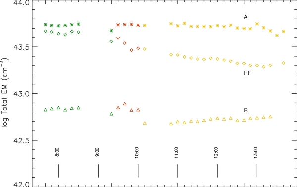
Figure 10. Temporal evolution of the total EM for the three regions: A (stars), BF (diamonds), and B (triangles). Green points correspond to data sets taken before the CME event, red points are taken during the CME passage in the EIS slit field of view, and yellow points are after the CME ejecta have left.
Download figure:
Standard image High-resolution image4.5.3. Are There Signatures of the CME Shock?
The increase in the hot component of the DEM closely follows the appearance of the CME core in the FOV of the B and BF regions. However, it is also interesting to note that in the BF data set the hot component of the plasma shown in Figure 9 appears 10 minutes before the CME core enters the EIS slit FOV. No sign of this behavior is found in data set B, and leads us to speculate that this might be a signature of the shock due to the CME front leaving the Sun before the CME ejecta. However, an inspection of the EIS spectrum before the CME core appearance does not reveal any feature that could be associated with the CME front, and there is no indication of velocities large enough to drive a shock. There is also no indication of the enhanced line widths seen in the spectra of CME-driven shock waves (e.g., Raymond et al. 2000).
4.6. Mass
A coarse estimate of the mass of the BF observed by EIS can be obtained using the measured electron density as well as an estimate of the volume. We assumed a unity filling factor. To determine the BF volume, we need to make some assumption on the depth of the BF plasma along the line of sight. Patsourakos & Vourlidas (2011) estimated that the CS shape was similar to a slab with a depth approximately one-third of the width, using the total brightness of the same CS obtained with the STEREO and SOHO coronographs above 2.2 R☉. We do not know whether and how such a depth is maintained at 1.1 R☉, very close to the XEA. We thus assumed two different shapes: a cylindrical structure and the slab geometry determined by Patsourakos & Vourlidas (2011). In the first case, the depth is assumed to be equal to the size of the BF along the EIS slit, and thus it is 130''–180'' (as shown in Figure 6, bottom). In the second case, the depth is taken to be one-third of this value: 40''–60''. The width of the slit is 2''or 0.0021 R☉.
The resulting BF mass estimates as a function of time are shown in Figure 6. Mass slowly decreases with time, due to the shrinking in the BF width, and it is around 1012 g, a value comparable to CS estimates by Vrsnak et al. (2009) after considering the LASCO pixel size and the size of the region shown in Figure 6. Uncertainties in Figure 6 are from the measured BF width and density, but not in the assumed filling factor and geometry, so that the present estimate is taken just as an indication of the order of magnitude of the BF mass.
Similar estimates cannot be made for data set B, even if they would help understand the role of the mass lost by the dimmed material in the overall mass of the CME. The problem is that there is no reliable estimate of the dimming region volume, since it is not possible to determine its extent along the line of sight and thus derive its mass. Also, no reliable density estimate can be made either, as the only ion providing density sensitive ratios with minimal background contamination is Fe xiv. However, Fe xiv ratios provide densities larger than those by Fe xiii by a factor of 5–10 before the CME eruption, due to the presence of an Fe x blend in the 264.79 Å line. Nevertheless, they show a significant decrease from pre-CME values in the B data set that can be ascribed to a density decrease. Thus, even if a reliable density measurement cannot be obtained, the Fe xiv ratio indicates a density decrease in the dimmed material.
4.7. Elemental Abundance
The relative abundance of high-FIP to low-FIP elements can be an important tracer of the origin of the BF plasma. However, it is not easy to determine with EIS, as the only element available in this data set whose FIP is larger than 10 eV is sulfur. In all spectra, regardless of position and time, the S abundance needed to be increased by a factor of 1.5–2.0 to match the abundance of elements with an FIP smaller than 10 eV from the assumed abundance of Feldman et al. (1992), which is only 15% larger than the photospheric abundance. The S correction may have two meanings: S is partially affected by the FIP effect and its abundance is increased over its photospheric values, or the S abundance might be photospheric, so that the FIP effect is less pronounced everywhere and thus the absolute abundance of the low-FIP elements needs to be decreased by a factor 1.5–2.0. In the latter case, the absolute value of all DEM curves needs to be increased by the same amount to reproduce the observed line intensities. If we define the "FIP bias" of a plasma as the amount of increase of low-FIP coronal abundance over the photospheric values, results show that everywhere the FIP bias is a factor of two to four. As a comparison, the standard FIP bias in the quiet corona is a factor of about four.
It is not easy to understand which of the two scenarios is the correct one. First, there are no other high-FIP ions available to check the correction to the sulfur abundance. Second, the amount of the sulfur FIP bias in the quiet corona is not well established. In fact, the sulfur's FIP is 10.4 eV, very close to the threshold traditionally associated with the FIP effect: it is not clear whether S should be considered a high-FIP or a low-FIP element and observations do not provide a clear picture. As an example, Feldman et al. (1998) report that the S abundance measured with SOHO/SUMER over a quiescent streamer is affected by an FIP bias between 1.2 and 2.0, while the rest of the low-FIP elements were biased by a standard coronal factor of four; on the contrary, the S abundance value in the coronal data set of Feldman et al. (1992) and in the photospheric data set by Grevesse & Sauval (1998) differ by less than 15%.
4.8. XRT Count Rates
We used the DEM curves calculated in each region at all times from the EIS data to predict the spectrum in the wavelength range where the XRT Al-poly filter is sensitive; we then folded the spectrum through the filter's wavelength response function to calculate the expected counts. We used the same element abundances adopted for the DEM determination, which had an FIP bias of four. Figure 11 shows the results. The observed count rates (in DN s−1) are shown in the bottom panels, corresponding to each selected region. The top panels show the observed to predicted ratio. The uncertainty in the XRT count rates combines the statistical and the calibration uncertainties, considering that XRT counts were averaged over wide regions to increase the signal-to-noise ratio. For the Al-poly filter, we conservatively assume a 20% uncertainty. The uncertainties tied to the synthetic spectrum, due to atomic physics and DEM uncertainties, are not included as they can be determined only with great difficulty; their effect is to further broaden the error bars.

Figure 11. Comparison of observed and predicted XRT counts for each of the selected regions, as marked on the top of each column. For each region, the top panel shows the observed to predicted count rate ratio, the bottom panel shows the observed XRT counts (DN s−1).
Download figure:
Standard image High-resolution image
Figure 11 shows that in each of the regions the predicted and observed count rates are in broad agreement. The predicted count rates for data set A are lower than the observed ones by about 20%–30% at all times. This could be due to two possible reasons: (1) the "A" data set includes small amounts of hot plasma whose emission is detected by XRT but is too small to produce spectral lines observable by EIS or (2) the relative calibration of EIS and XRT is offset by that amount. Given the uncertainties involved in the calibration of the predicted XRT counts and in the DEM determination, we feel that this disagreement, while present, is too small to allow any conclusion on these two possibilities.
The observed and predicted ratios in the BF and B data sets agree in uncertainties, and this indicates that the long-term effect of the passage of the CME is limited to producing plasmas at temperatures around or below 4 MK. No additional, hotter component is needed to reproduce XRT observations. It is interesting to note that the bump in the Fobs/Fpred ratio in the BF data set between 11 UT and 12 UT may be really due to an additional hotter plasma component not detected by EIS. However, uncertainties prevent us from making meaningful measurements of the properties of such additional plasma.
The only significant differences (within a factor of two) are only found during the CME event itself, where XRT emission exceeds predictions. The time difference between the disagreements in the two data sets is consistent with the passage of a hot feature trailing the CME core, where an additional plasma component is needed, as noted by Landi et al. (2010). This will be studied in a future paper (E. Landi et al. 2012, in preparation).
We also tested the effect of the uncertainty in the element composition by lowering the abundances of the low-FIP elements by a factor of 1.5 and increasing the DEM value by the same factor. These corrections correspond to using a set of abundances with an FIP bias of ≃ 2.5 and photospheric sulfur abundance. Depending on the selected regions, the predicted count rates increase by an additional factor of 1.3–1.5, removing the discrepancy in data set A and worsening the agreement found in the other two data sets. The disagreement in the Fobs/Fpred ratios that the FIP bias of 2.5 introduces in data sets BF and B seems to indicate that the FIP bias is indeed four. However, since there is no independent determination of the absolute abundance of the plasma, we consider the factor 1.3–1.5 as an additional uncertainty in the calculation of the expected XRT count rates. Thus, we conclude that there is no firm evidence of additional plasma components at high temperatures neither in the BF plasma nor in the B plasma, both heated after the CME event.
5. DISCUSSION
The first question that needs to be answered is the nature of the XEA and its relationship to the CS. Most importantly, does the XEA plasma belong to the PEA that is formed in the wave of the CME ejection? The first thing to note is that the XEA plasma decreases with height and time, as shown in Figure 1. This is not unexpected in PEA loops; for example, Lin (2004) showed that even if the height of the lower end of the CS increases with time as reconnection continues, the individual PEA loops formed at that lower end decrease their height. Since loops formed later in time are made of less dense (and thus less bright) material, it is not unexpected that the overall PEA may seem to shrink in time. However, the decisive point to interpret the XEA is the fact that the height of the lower end of the CS is nevertheless predicted to rise with time. There are two possibilities: either this point is located above the height of the EIS slit FOV from the beginning, or it was located below it. However, in the former case the EIS slit would never cross the CS; on the contrary, Figure 1 clearly shows that after 13:00 UT the CS is visible and crosses the EIS slit. This means that the lower point of the CS lies below the EIS slit for the entire duration of the EIS observations. As a consequence, the PEA is expected to be located below the EIS slit all the time, so that the XEA plasma is not related to the PEA at all. We can interpret the XEA plasma as a loop arcade that has been formed during, or displaced by, the CME eruption. Then it shrinks with time and dominates the emission along the EIS slit only up to 13:00 UT.
When comparing the present results for the CS with those obtained in previous works, we need to bear in mind that all those measurements were obtained at larger heights than the present ones. Only Innes et al. (2003) and Wang et al. (2007) analyzed observations at similar heights as the present one. These differences in height can result in large differences in each of the physical properties we compare. Thus, we will highlight only the general trends rather than make a direct comparison.
First, we found that the element abundances of the BF are the same as those in the ambient plasma. Even if we were not able to determine the absolute value of the FIP bias for the plasma (whether it was 2 or 4), the fact that the composition was the same as in the background corona is in line with the abundance determination by Ciaravella et al. (2002), Ko et al. (2003), and Bemporad et al. (2006), who found that the CS plasma composition was not photospheric, and its FIP bias ranged between 3 and 8, thus indicating a coronal origin of the CS material.
The thickness of the CS is generally expected to be less than 0.001 R☉, and in the Petschek reconnection picture, it is expected to increase with distance away from the X-line, as is shown in the measurements of Vrsnak et al. (2009). The size of the CS determined by EIS, as seen in Figure 6, is around 0.13 R☉. This value is compatible with the estimate made by Patsourakos & Vourlidas (2011), who report 0.05 and 0.15 R☉ for the thickness and depth of the CS in this event using LASCO C2 and SECCHI COR2-A at heights larger than the EIS ones. As a comparison, UVCS has reported thicknesses of 0.04–0.08 R☉ (Ciaravella & Raymond 2008) and ∼0.3 R☉ (Lin et al. 2005) or larger, though the larger sizes are affected by binning of the data, and they may refer to the depth rather than the thickness. On the contrary, Savage et al. (2010) report 0.005 R☉ as the size from the XRT images. The large difference between this estimate and all other results including our own is due to the fact that Savage et al. (2010) measured the apparent size of a sharp spike within the bright feature in the XRT image, while we report the full size of such a feature (see Figure 5). Savage et al. (2010) identify the spike seen in XRT as the "active" part of the CS, while no clear corresponding feature stands out in the emission line image. There are two things to note. First, by determining the width of the entire feature rather than of a single spike, we overestimated the true width of the CS. In other words, we measured the upper limit of the CS size. Second, Figure 4 shows that before 14 UT, there is no clear boundary between the CS and the post-CME loops even if images seem to show it (see Figure 1), and thus we felt it safer to report the width of the entire BF rather than concentrate on a small spike.
We found that the plasma in the BF does not harbor detectable flows along the EIS line of sight. This result contradicts the measurements made by Savage et al. (2010), who find velocities of 90–120 km s−1. Considering the 24° inclination of the CS relative to the plane of the sky, such velocities are expected to generate detectable Doppler shifts in the EIS spectra. The reason for this discrepancy is not clear. First, it is possible that the inclination angle is smaller than 24°. However, even if this angle were 10°, detectable Doppler shifts would still be expected. Second, XRT might be observing patchy reconnection that affects X-ray emission enough to be detected and interpreted as a motion. Third, the plasma observed by EIS mostly belongs to the post-CME loops where flows, if any, may be completely unrelated with those in the CS observed by Savage et al. (2010).
The temperature given by the DEM of the CS and XEA in this event is cooler than the temperatures inferred from the UVCS and SUMER observations of CSs. Those observations showed ions such as Ca xiv, Fe xviii, and Fe xxi, whose contribution functions peak at temperatures well above the 3 MK we infer from EIS and XRT observations. This is largely a selection effect in that the Fe xviii line, which is not normally present in UVCS spectra, was the signature used to identify CSs in the UVCS observations so that UVCS may be observing hotter CS than the present one. It may also be that the UVCS observations generally pertained to faster CMEs. One might expect that the CME speed is related to the Alfvén speed, and that the transformation of magnetic energy to heat gives a temperature related to the Alfvén speed squared. The CDAW CME catalog gives a speed of 650 km s−1 for the event considered here, while the speeds of the UVCS events were 430, 1800, 1700, 980, and 2600 km s−1 for the 1998 March 28 and 2002 January 10 events, two events on 2003 June 2, and the November 4 events, respectively.
The CS electron density was found to be constant with time by Bemporad et al. (2006) and Schettino et al. (2010), and we confirm such a behavior in our measurements where we do not see the decrease with time found by Ciaravella & Raymond (2008). We also find that the temperature structure of the CS is rather stable, as the DEM curves and relative importance of plasma hotter than log T = 6.2 are rather constant in time after the CS has formed (Figure 9). This behavior disagrees again with the temperature decrease found by Bemporad et al. (2006), Ciaravella & Raymond (2008), and Schettino et al. (2010).
The most remarkable result of our analysis is the low density derived from the Fe xiii line ratio. In fact, theoretical models predict the CS density to be larger than the surroundings due to slow mode shocks in the classical Petschek picture. Our low density value is also in contrast with the value found by Patsourakos & Vourlidas (2011) at larger heights than those considered here. The only previous density determination that did not rely on an assumed geometry and filling factor is that of Ciaravella & Raymond (2008), who found densities of (0.4–1) × 108 cm−3 at 1.7 R☉ in a far more energetic event. In that event and others observed by UVCS and LASCO, the density in the CS was two to three times the density in the surrounding corona. However, this result can be understood if we think that the density of the CS is compared to the density of the background and foreground plasma along the line of sight rather than to the density of the much fainter, dimmed plasma closest to the CS. Unfortunately, we do not have a reliable line ratio with which to measure the density of the latter because the emission of the plasma immediately around the CS is much fainter than that of the plasma along the entire line of sight.
Our results show that the CD that forms in the aftermath of the CME event consists of three main features: a net loss of total EM, a large loss of plasma at ambient coronal temperatures, and the heating of plasma to temperatures up to 3 MK. Thus, the plasma in region B must have indeed contributed to the total mass of the CME, as suggested by most of the earlier results, although the lack of reliable density and volume estimates prevent us from determining the size of such contribution.
Another notable result is that we do not observe any Doppler shift in the B data set after the CME left the EIS FOV. Thus, we cannot determine whether and to what extent the plasma emitting the spectra we study is a leftover of the plasma present before the eruption, which has been heated by the CME passage, or is made of plasma transported from below and heated up to 3 MK. The lack of Doppler shifts seems to indicate the heating of local plasma as the most likely origin of the hot CD plasma, but the continuous replenishment that increases the EM seems to indicate that undetected flows may be active in bringing new material in the EIS FOV. It is interesting to note, however, that the DEM shape of the dimmed material does not change in time, so that the inflowing material thermal structure is the same as that of the CD.
6. CONCLUSIONS
In this paper we measured the physical properties of a loop arcade formed in the active region after the CME eruption (XEA), a CS, and CD plasmas that were observed as part of the 2008 April 9 CME event. We used a time series of EIS spectra and XRT images to determine the main physical properties of the emitting material and monitor their evolution during the first three hours after the CME. We found the following results.
- 1.The physical properties of the CS and XEA plasmas are very similar.
- 2.We provide an upper limit to the size of the CS, which is larger than the estimates by Savage et al. (2010) and more consistent with earlier UVCS and LASCO CS sizes.
- 3.The temperature of the XEA and CS plasmas never exceeds 3 MK and is fairly stable with time. Any additional contribution to XRT count rates from plasma at temperatures higher than 3 MK, if any, is small.
- 4.The electron density in the XEA and CS plasmas is fairly stable with time and is lower than in the background plasma by a factor of about 1.5–2. No direct measurement of the density of the surrounding material is available, but there are indications that it is lower than the density in the background, XEA and CS plasmas.
- 5.The composition of the arcade loop and CS plasmas is the same as the composition of the ambient plasma, indicating that the material from the former comes from the corona. The EIS spectrum did not include enough lines that allowed us to determine the FIP bias with accuracy, but the observations are compatible with an FIP bias of ≈2–4.
- 6.The CD consists of a net decrease of plasma, a large decrease of plasma at ambient coronal temperatures, and an increase of plasma heated to temperatures up to 3 MK. Its EM slowly increases with time, indicating that plasma at all temperatures is flowing into the region even if we cannot measure its velocity.
- 7.The mass of the XEA and CS plasmas is very difficult to measure; estimates done using different assumptions in the geometry of the structure and unity filling factor indicate that it lies in the (1–3) × 1012 g range.
- 8.This event shows an enhanced level of unresolved motions in the CD material.
This set of results complements those obtained at larger heights by Savage et al. (2010) and Patsourakos & Vourlidas (2011) for the same event, and, when coupled to the measurements of the physical properties and evolution of the CME core made by Landi et al. (2010), provides the most comprehensive set of observations ever made on the same CME event, which can be used as a test for theoretical models.
The work of E. Landi is supported by NNX10AM17G, NNX11AC20G, and other NASA grants. The work of M.P.M. is supported by several NASA grants. The work of J.C.R. is supported by NASA grant NNX11AB61G to the Smithsonian Astrophysical Observatory. Hinode is a Japanese mission built and launched by JAXA/ISAS, collaborating with NAOJ as a domestic partner, and NASA (USA), and PPARC (UK) as international partners. We warmly thank the anonymous referee who helped us improve our original manuscript considerably.