


ABSTRACT
Carbon-enhanced metal-poor (CEMP) stars are believed to show the chemical imprints of more massive stars (M ≳ 0.8 M☉) that are now extinct. In particular, it is expected that the observed abundance of Li should deviate in these stars from the standard Spite lithium plateau. We study here a sample of 11 metal-poor stars and a double-lined spectroscopic binary with −1.8 < [Fe/H] < −3.3 observed with the Very Large Telescope/UVES spectrograph. Among these 12 metal-poor stars, there are 8 CEMP stars for which we measure or constrain the Li abundance. In contrast to previous arguments, we demonstrate that an appropriate regime of dilution permits the existence of "Li-Spite plateau and C-rich" stars, whereas some of the "Li-depleted and C-rich" stars call for an unidentified additional depletion mechanism that cannot be explained by dilution alone. We find evidence that rotation is related to the Li depletion in some CEMP stars. Additionally, we report on a newly recognized double-lined spectroscopic binary star in our sample. For this star, we develop a new technique from which estimates of stellar parameters and luminosity ratios can be derived based on a high-resolution spectrum alone, without the need for input from evolutionary models.
Export citation and abstract BibTeX RIS
1. INTRODUCTION
Observations of the most metal-poor stars in the Galaxy offer the opportunity to study the earliest star formation episodes, either through the nucleosynthesis that polluted the stars under study or through the characteristics of the surviving stars themselves. One of the striking observational facts established through extensive surveys for metal-poor stars (most notably, the HK survey, Beers et al. 1992, and the Hamburg/ESO Survey, Christlieb et al. 2008) is the large number of C-rich stars, with as much as 25% of the stars with [Fe/H] <−2.5 having [C/Fe] > +1.0 (Lucatello et al. 2005a, 2006). The origin of these carbon-enhanced metal-poor (CEMP; Beers & Christlieb 2005) stars is important for understanding conditions in the early universe, because the competing theories predict pollution from different nucleosynthetic sources. Some CEMP stars are enhanced in the "slow neutron-capture" (the s-process) elements, whereas other CEMP stars are also enhanced in the "rapid neutron capture" (the r-process) elements. The s-process elements are produced primarily in low-mass asymptotic giant branch (AGB; e.g., Herwig 2005) stars, while the r-process likely occurs in explosive events such as core-collapse supernovae (SNe; see review by Sneden et al. 2008). CEMP stars with a pure s-process signature are classified as CEMP-s; the subset of CEMP-s stars that possess evidence for the addition of r-process elements are referred to as CEMP-rs (CEMP-r/s in the original nomenclature of Beers & Christlieb 2005). Thus far, only a single example of a CEMP-r star (a class that exhibits pure r-process enrichment, with no apparent contribution from the s-process) has been identified, CS 22902-052 (Sneden et al. 2003). A final class, the CEMP-no stars, exhibit no enhancements in the neutron-capture elements compared to the average non-C-rich metal-poor stars in the Galaxy (Beers & Christlieb 2005).
Many CEMP stars exhibit radial velocity variations, indicating that they are members of multiple systems such as binaries. A statistical analysis of radial velocity variations (Lucatello et al. 2005b) and agreement between the observed abundances of neutron-capture elements and the predictions of s-process production in AGB stars (e.g., Masseron et al. 2010) indicate that the CEMP-s stars are likely to have all been created by mass transfer from an AGB companion star. Models for the pollution of the CEMP-rs stars are more uncertain, because the source of some of their elements, such as Eu, is unclear. Several theories have been proposed that tie the production of the s-process and the r-process together, including accretion-induced collapse of a white dwarf (see review in Jonsell et al. 2006). Similarly, the CEMP-no abundance patterns have been suggested to arise from a number of alternative scenarios. Proposals for their formation include pollution by a failed SN (Umeda & Nomoto 2003), winds from the surface of massive, rapidly rotating, mega- metal-poor ([Fe/H] <−6.0) stars in the early universe (Hirschi 2007), or by an AGB companion that produced little or no s-process elements (Suda et al. 2004; Masseron et al. 2010).
The Li abundances of CEMP stars are interesting to consider; when compared with the predictions of theories of C-production, the Li abundances of some CEMP stars exhibit unexpected results. In non-C-rich, metal-poor stars, stars within a narrow mass range have sufficiently small convective envelopes that they preserve most of the Li that was present in the gas clouds from which they formed, although some Li may be lost to diffusion and turbulent mixing (e.g., Richard et al. 2005; Meléndez et al. 2010). These stars define the Spite plateau (Spite & Spite 1982) and are at or near the main-sequence turnoff in a metal-poor population. As stars leave the main sequence and become subgiants, the Li preserved in their outer atmospheres is diluted when it is mixed with material from deeper in the stellar envelope, where the Li has been burned. As the convective envelope deepens and Li is carried down to temperatures high enough to burn, the stellar envelope becomes increasingly Li-poor.
Lithium may be produced during the AGB phase by the Cameron–Fowler mechanism, where 7Be is created at the bottom of the convective envelope and captures an electron. The resulting Li is carried to the cooler upper layers of the star before the 7Li is destroyed by proton capture (Sackmann & Boothroyd 1992). Gas containing this Li can be released into the interstellar medium (ISM) when the AGB star loses mass. However, the predicted production strongly depends on model assumptions, in particular on the adopted convection parameterization and mass-loss recipe. Studies of the red giant branch (RGB) show that extra-mixing mechanisms can possibly lead to Li production (Denissenkov & Herwig 2004), and such extra-mixing mechanisms undoubtedly exist during the AGB phase as well (e.g., cool bottom processing, Nollett et al. 2003; Domínguez et al. 2004; or thermohaline mixing, Stancliffe 2010; Charbonnel & Lagarde 2010). Overall, existing yields for Li from AGB models show a strong mass dependence (see Figure 1), and in general, the Li/H ratio in AGB yields is smaller than the Spite plateau (e.g., Karakas 2010; Ventura & D'Antona 2010). Models of AGB stars with a range of masses show that Li is produced at abundance levels greater than the Spite plateau over a limited mass range (Figure 1). For the Karakas models, this is M ∼ 3 M☉, while Ventura & D'Antona (2010) find strong Li production only in the most massive (M > 7 M☉) AGB stars. The Ventura & D'Antona yields and the Karakas yields are for two different metallicities, which might explain part of the discrepancy. A simple prediction would be that if the CEMP stars were polluted by AGB stars, the Li abundances of the CEMP stars should reflect the fact that Li yields from AGB stars have been dumped on them. Another expectation would be that the Li and C+N abundances in such stars could be used to constrain nucleosynthesis in low-mass, low-metallicity AGB stars. However, although models accounting for binary interactions are being developed (e.g., Siess et al. 2011), it must be stressed that the impact of the presence of a companion on AGB nucleosynthesis and in particular Li yields is currently not well constrained. In the pollution coming from rotating massive stars, some Li depletion is expected (as well as carbon enhancement). Unless the synthesized material is mixed with a large amount of the surrounding ISM, log (Li) will be less than 2.0 (Meynet et al. 2010).

Figure 1. Top panels: Li yields as a function of AGB mass from Karakas (2010; left panel) and from Ventura & D'Antona (2010; right panel). The dotted line represents the Spite Li plateau as observed in non-CEMP stars. Bottom panels: the [C/N] ratio as a function of AGB mass for the same models. The shaded area indicates the region where hot bottom burning occurs, which leads to the production of N-rich rather than C-rich stars and therefore will not result in the formation of CEMP stars.
Download figure:
Standard image High-resolution imageThe strongest Li line is the doublet at 6707 Å, a much longer wavelength than most of the atomic lines that are of interest in CEMP stars. Therefore, in the case of many observations carried out to date, the Li line was not covered in the observed part of the spectrum (or the observations were of insufficient quality to measure this weak feature); thus, Li measurements for CEMP stars are somewhat limited. Norris et al. (1997a) discussed the Li measurements of Thorburn & Beers (1992) and Thorburn (1994) for the CEMP stars LP 625-44, LP 706-7, CS 22898-027, and CS 22958-042. Both LP 625-44 and CS 22958-042 have Li abundances lower than non-CEMP stars at a similar evolutionary state, but LP 706-7 and CS 22898-027, both near the turnoff, have Li abundances very close to the Spite plateau. The Li abundance in LP 706-7, log(Li) = 2.25, is slightly below the plateau values, taken by Thorburn (1994) to be log(Li) = 2.32, while CS 22898-027 is Li-rich relative to the plateau, with log(Li) =2.52. Observations of CH stars, which are the result of AGB mass transfer in moderately metal-poor ([Fe/H] ∼−1) binary systems (McClure 1984), show that they are Li depleted (Smith et al. 1993). Therefore, Norris et al. (1997a) argued that a Li abundance near the plateau was evidence against the binary hypothesis. Other CEMP stars with Li abundances near the Spite plateau are SDSS J1036+1212 (log(Li) = 2.21; Behara et al. 2010) and CS 31080-095 (log(Li) =1.73) and CS 29528-041 (log(Li) =1.71), both from Sivarani et al. (2006).
One extremely interesting additional example of CEMP stars with Li abundance measurements near the Spite plateau is the double-lined spectroscopic binary CS 22964-161 (Thompson et al. 2008). The working hypothesis offered by these authors to account for their observations is that the AGB star was a member of a triple system and polluted the other two stars. They argued that the Li abundance (log(Li) = 2.09) had to be the result of Li in the mass transferred from the AGB star, because otherwise the pollution by Li-free material would lower the abundance to below the plateau value (log(Li) = 2.10, Bonifacio et al. 2007). Based on fits of predicted AGB yields to the observed abundances of the neutron-capture elements, the authors argued that the polluting AGB star had M < 2 M☉. Because this mass is not expected to produce Li by the Cameron–Fowler mechanism in standard models, they suggested two possible Li production mechanisms that could work in low-mass AGB stars. In an H-flash episode, the temperature in the He intershell region can reach high enough temperatures to produce Li (Iwamoto et al. 2004). Cool bottom processing might also be responsible for increased Li production in low-mass stars (Domínguez et al. 2004). Examples of Li-depleted CEMP turnoff stars also continued to be found, for example, CS 22958-042 (Sivarani et al. 2006) and the most iron-poor ([Fe/H] =−5.4) and highest [C/Fe] star ([C/Fe] = +4) HE 1327-2326, with Li abundance log(Li) < 0.62 (Frebel et al. 2008), a significant upper limit well below the Spite plateau. We finally note that there is one remarkable metal-poor giant, the CEMP-rs star HKII 17435-00532 with a Spite Li plateau abundance analyzed by Roederer et al. (2008). Because Li must be depleted after the first dredge-up, they claim that in situ Li production is required in order to explain such a high observed abundance.
Observations of Li abundances in CEMP stars have therefore established that there exists a spread in Li values, even among the turnoff stars. It is an open question if this spread can be reconciled with the binary AGB mass transfer scenario, or if the carbon in these stars comes from a different source that does not require the presence of an AGB companion.
An additional complication for understanding Li abundances in C-rich stars are processes that occur in the CEMP star itself that could change the surface abundances of Li, independently of stellar evolution. Stancliffe et al. (2007) showed that, because CEMP stars have accreted material that has been enhanced in AGB nucleosynthesis products, an additional mixing process below the conventional stellar atmosphere of main-sequence stars should occur, the so-called thermohaline mixing. Thermohaline mixing could affect both the surface Li and C abundances if the mixing reaches sufficiently deep into the star. Rotation is another efficient way to alter the surface abundance of Li, where additional meridional circulation and shear turbulence could destroy Li (see, e.g., Talon & Charbonnel 2005, and references therein).
This paper is organized as follows. In Section 2, we briefly review the abundance analysis techniques for the single-lined spectra in our sample. One of our stars is a double-lined spectroscopic binary, and we devote Section 2.2 to presenting a new technique for the analysis of such systems. This technique avoids the use of isochrones in measuring the properties of the primaries and secondaries from a single spectrum. In Section 3, we present the Li abundances and carbon isotope ratios for our program stars. We also calculate the impact on the observed Li abundance if material from the AGB star is mixed with material in a CEMP star and compare with observations from our sample and the literature. Section 4 briefly summarizes our conclusions.
2. OBSERVATIONS AND DATA ANALYSIS
We observed 13 stars with Very Large Telescope (VLT)-UVES (Dekker et al. 2000), under ESO program 076.D-0451A, in service mode during 2005 October–2006 March. The sample was chosen from the known CEMP stars in the literature available for observation from the southern hemisphere. Our goal was to measure the Li abundance and the 12C/13C ratio, so we used the 390+580 nm setting, which resulted in wavelength coverage of 3215 Å to 6815 Å. We tried to include as many warm CEMP stars as possible, as well as a range of CEMP classes, but because of the limited number of available CEMP targets, some stars cooler than ideal were observed. The spectra have a high resolution (R ∼ 45,000) and a high signal-to-noise ratio (S/N ∼ 100 per pixel). We re-reduced the UVES pipeline data, following the procedures of Masseron (2006), to obtain the best possible S/N in the final spectra.
2.1. Model Atmospheres and Linelists
Our analysis was done using the TurboSpectrum code by Alvarez & Plez (1998). Temperatures and gravities were derived using standard spectroscopic techniques: abundances independent of excitation potential for Fe i lines and ionization equilibrium between Fe i and Fe ii lines, respectively. Effective temperatures were also inferred by fitting the wings of the Hα Balmer lines. Microturbulence velocities were determined by requiring no trend for the abundances of Fe i lines versus their equivalent widths. The log gf values for Fe are identical to those of Hill et al. (2002). Because CNO abundances may have a strong impact on the structure of the stellar atmospheres (Masseron 2006), 1D MARCS models (Gustafsson et al. 2008) have been built specifically for each star, taking into account the peculiar abundances. The final stellar parameters are listed in Table 1.
Table 1. Stellar Parameters and Abundances
| Star | Teff | log g | [Fe/H] | ξ | log(O) |
log(Li) |
log(C) |
12C/13C |
|---|---|---|---|---|---|---|---|---|
| (K) | (km s−1) | |||||||
| CEMP Stars | ||||||||
| CS 22183-015 | 5450 | 3.0 | −2.87 (0.15) | 1.5 | <7.5 | <0.7 | 7.9 (0.05) | 7 (1) |
| CS 22887-048 | 6500 | 3.7 | −1.80 (0.16) | 1.8 | <8.0 | <1.4 | 8.1 (0.05) | 3 (0.5) |
| CS 22898-027 | 6000 | 3.5 | −2.49 (0.17) | 1.4 | <7.6 | 2.18 (0.1) | 8.0 (0.05) | 12 (2) |
| CS 22947-187 | 5200 | 1.5 | −2.56 (0.09) | 1.9 | 6.8 (0.2) | <0.5 | 6.95 (0.05) | 3 (0.5) |
| CS 22949-008a | 6300 | 4.0 | −2.14 (0.04) | 1.5 | ... | <1.0 | 7.85 (0.05) | >30 |
| CS 22949-008b | 5300 | 4.7 | −2.14 (0.04) | 1.5 | ... | <1.0 | 7.85 (0.05) | >30 |
| CS 29512-073 | 5600 | 3.4 | −2.09 (0.14) | 1.3 | <7.6 | 1.93 (0.1) | 7.55 (0.05) | >60 |
| CS 30322-023 | 4100 | −0.3 | −3.33 (0.19) | 2.2 | 5.9 (0.1) | <−0.3 | 5.6 (0.05) | 4 (0.5) |
| HD 198269 | 4500 | 1.0 | −1.84 (0.25) | 1.8 | ... | <0.2 | 7.45 (0.05) | 5 (1) |
| Metal-poor Stars | ||||||||
| CS 22948-104 | 5000 | 2.3 | −2.76 (0.11) | 1.6 | <6.7 | 0.92 (0.1) | 6.05 (0.05) | >50 |
| CS 29493-090 | 4700 | 0.9 | −3.25 (0.15) | 1.6 | 6.3 (0.2) | <−0.2 | 5.95 (0.05) | 6 (1) |
| CS 29517-025 | 5300 | 1.2 | −2.57 (0.09) | 2.0 | <6.9 | <0.5 | 6.0 (0.05) | ... |
| CS 30312-100 | 5000 | 2.0 | −2.70 (0.11) | 1.5 | 6.9 (0.2) | 0.85 (0.1) | 6.08 (0.05) | >50 |
Download table as: ASCIITypeset image
The abundances of Li, C, N,O, Na, Mg, Ba, Eu, and the C isotope ratios were measured in these stars using synthesis comparisons for all elements except Fe, because CEMP-star spectra are usually blended with molecular features. When observable, O was first determined via the O forbidden line at 630 nm (log gf = −9.750), in order to ensure proper chemical equilibrium of the C-based molecules. If O was not observable, or was strongly blended by a telluric line, a value of [O/Fe] = +0.4 was assumed. The C and N abundances and the 12C/13C ratios were then measured, using unsaturated CH, CN, and NH lines (B. Plez 2008, private communication). Simultaneously, Na abundances were measured using the Na i lines at 3302 Å and 5682–5688 Å, and Mg abundances using the Mg i 4057–4167-5528–5711 Å lines. Atmosphere models and abundance determination have been iterated until convergence, because their deviation from standard composition implies changes in the structure of the stellar atmosphere. The abundances of Ba and Eu were then obtained, including hyperfine structure and isotope shifts; the atomic data have been taken from Masseron et al. (2006) and Lawler et al. (2001), respectively. Finally, we measured Li (adopting the linelist of Hobbs et al. 1999), assuming that the 6Li/7Li ratio is the solar value (0.08). We adopt the solar photospheric abundances of Asplund et al. (2005) to calculate the abundance ratios relative to the Sun. Random errors are presented in parentheses in the tables and may be attributed to uncertainties in the continuum placement, to the noise of the observations, and to errors in the log gf values of the lines.
2.2. Spectroscopic Analysis of the Double-lined Binary
Among our sample, one star (CS 22949-008) is a double-lined spectroscopic binary (or SB2). Four SB2s composed of metal-poor stars ([Fe/H] <−1.5) have previously received extensive discussions in the literature: CS 22873-139, first analyzed by Preston (1994) and later re-observed by Spite et al. (2000); CS 29527-015, studied by Thorburn (1994) and Norris et al. (1997a), with the Li detection by Spite et al. (2000); CS 22876-032, studied by Norris et al. (2000) and González Hernández et al. (2008); and CS 22964-161, analyzed by Thompson et al. (2008). As mentioned in the Introduction, the latter system exhibits a large C enhancement, similar to that of our system.
A proper abundance analysis of such a system requires deriving the four parameters (Teff, log g, metallicity, microturbulence, as well as the convolution profile for proper synthesis) of the two components of the binary based on information extracted from a single spectrum. To successfully separate the two stars, the luminosity ratio of the two stars must also be determined. Standard methods (e.g., Thompson et al. 2008) usually make use of isochrones to determine this ratio. However, thanks to the large wavelength coverage of our data, we can derive the stellar parameters for each component, as well as their luminosity ratio, using only a single high-resolution spectrum, as described in this section.
2.2.1. Principles
By taking into account the veiling flux (FBR2B) of star B, the observed equivalent width EWobs for star A can be expressed such that EWobsA × (FAR2A + FBR2B) = EWA × FAR2A, where Fλ, i is the continuum flux at the wavelength λ of star i, EWA is the computed equivalent width for star A, and Ri is the radius of star i. This formula can be then rearranged the following way:

(and reciprocally for component B).
While EWobsi can be directly measured on the spectrum (if the radial velocity shift between the two components is sufficiently large), Fλ, i and EWi can be computed from synthetic spectra for any effective temperature, gravity, metallicity, and microturbulence. Note that using equivalent widths offers the advantage of being independent of the instrumental, macroturbulent, or rotation profile. These profiles can be derived by synthetic comparison once all the other parameters have been set.
Moreover, Equation (1) shows that the appropriate combination of these factors should be constant, as (RB/RA)2 represents the radius ratio of the stars. This property can be used to derive the stellar parameters of the individual components of an SB2. In particular, (RB/RA)2 must be independent of the excitation potential of the spectral lines. As is the case in the analysis of single-star spectra, the dependence of EWA on excitation potential is mostly sensitive to changes in effective temperature. Thus, by requiring no trend of (RB/RA)2 on excitation potential, we can constrain the effective temperature of each star.
In addition, the term Fλ, A/Fλ, B in Equation (1) is dependent on wavelength. Figure 2 illustrates how the contribution of the flux can vary over the spectrum, depending on its effective temperature. Hence, effective temperatures can be constrained by requiring no dependence of Equation (1) with wavelength instead of excitation potential. Because of the dependence of Equation (1) on excitation potential and wavelength and also on the continuum flux of the other component (i.e., its effective temperature), the temperature determination process must be iterated until convergence.

Figure 2. Example of the variation of the continuum flux distribution with wavelength for each component of an SB2, for three temperatures of the secondary, with the radius ratio and the temperature of the primary fixed to the case of the SB2 CS 22949-008. The discrepancy between the red and the blue portion of the contribution of the secondary flux to the total flux (lower panel) is more pronounced for the coolest temperatures.
Download figure:
Standard image High-resolution imageHowever, there is no constraint in Equation (1) on the abundance. Consequently, the derived radius ratio from this equation is dependent on the metallicity, as illustrated in Figure 3. Assuming that the metallicity is identical for both components, the radius ratio and the metallicity of the system can then be immediately derived simultaneously by choosing the metallicity that gives the same radius ratio for both the primary and secondary EWs. Without this assumption, Equation (1) is completely degenerate between the ratio of the metallicities of each component and the radius ratio. In this case, additional constraints on the radius ratio may be set from their observed orbital motion, or constraints on metallicity may be derived from another element.

Figure 3. Variation of the radius ratio with metallicity, using Equation (1) in the case of the SB2 CS 22949-008, with either the primary's (blue line) or the secondary's (red line) EWobs. The uncertainty on the radius ratio (shown with dotted lines) is due to the observed scatter in the equivalent widths. The shaded areas indicate the subsequent error on the derived metallicity. There is a dependency of the radius ratio on the metallicity.
Download figure:
Standard image High-resolution imageOnce the effective temperatures of the secondary and the primary, as well as the radius ratio, have been fixed, the veiling factor fλ, i = EWi/EWobsi can be computed for any set of lines. Hence, the respective EWi of individual stars can be recovered and standard techniques applied. Thus, gravity can be determined from the ionization equilibrium, as is usually done. Similarly, microturbulence velocity can be set by comparing the abundances of strong and weak lines. Note that Equation (1) is also dependent on the microturbulence, thanks to EWA, and the stellar parameter determination for the components has to be iterated until convergence.
In principle, this method should be applicable to any SB2 for which a spectrum with high resolution and a large wavelength range is available, with the minimum condition that the radial velocity shift is sufficiently large to permit the measurement of the equivalent widths of each component separately. In fact, this technique could even be extended to any SB2 spectrum, once constraints are known (or adopted) on the metallicity ratio or radius ratio of the components.
2.2.2. Application to CS 22949-008
We have applied the above technique to our double-lined spectroscopic binary CS 22949-008, using a set of measured equivalent widths for the Fe i lines. The derived parameters are listed in Table 2, with errors derived from the line-to-line scatter (one standard deviation). It may be counterintuitive that the error on the effective temperature of the secondary is better constrained than that of the primary. However, as illustrated in Figure 2, a change of 250 K in the temperature of the secondary leads to a change of 5% in its flux contribution to the total flux. Since the S/N of our spectrum is typically 100, it follows that the precision of the flux is known as well as 1%. Hence, a precision of ≈50 K for the temperature of the secondary can be achieved, while the uncertainty of the temperature of the primary is similar to literature values, because it is essentially dominated by the uncertainty on the spectral line data.
Table 2. CS 22949-008 Parameters
| Primary | Secondary | |
|---|---|---|
| Teff(K) | 6190+130− 150 | 5250+50− 50 |
| log g | 4.0 ± 0.2 | 4.7 ± 0.3 |
| ξt (km s−1) | 1.5 ± 0.3 | 1.3 ± 0.5 |
| [Fe/H] | −2.14 ± 0.04 | |
 |
0.59 ± 0.07 | |
 |
0.18 ± 0.04 | |
Download table as: ASCIITypeset image
Table 3 lists the systematic errors on the derived parameters of the SB2 due to uncertainties in the atmospheric parameters of each component. It is noticeable that changes in the stellar parameters of the primary do not impact on the determination of the parameters of the secondary. Indeed, the temperature of the secondary is strongly dependent on the wavelength, whereas a change in temperature of the primary acts as an almost constant change in the luminosity flux over wavelength; thus, it has little impact on the temperature determination. Overall, the technique we employ allows us to estimate the stellar parameters of CS 22949-008 fairly precisely. However, we emphasize that there is a relatively large contrast in effective temperature between the two components, such that Equation (1) is mostly sensitive to excitation potential in the case of the primary, whereas it is mostly sensitive to wavelength variation for the secondary. Hence, the derivation of stellar parameters for the two components is quite independent of one another. Indeed, the degeneracy that can be lifted in the analysis of our system, with a rather large contrast in temperature, is likely more robust than for systems with similar temperatures of the components.
Table 3. Error Budget for CS 22949-008
| Primary | Secondary | |||
|---|---|---|---|---|
| Teff + 150 K | ξt+0.5 | Teff + 150 K | ξt+0.5 | |
 |
+150 | +0.5 | +15 | 0 |
 |
+16 | 0 | +150 | +0.5 |
| Δ[Fe/H] | +0.11 | −0.06 | +0.02 | −0.01 |
 |
−0.053 | +0.015 | −0.007 | −0.014 |
 |
+0.02 | −0.01 | −0.02 | +0.01 |
Download table as: ASCIITypeset image
Figure 4 presents examples of the Fe i line fits. The radial velocity shift between the two stars is 25 km s−1. From this fit, convolution profiles have been set to 12 km s−1 for the primary star and 6 km s−1 for the secondary star.

Figure 4. Fit to the Fe i lines of the combined spectrum of the SB2 CS 22949-008. The thick black line shows the observed spectrum, while the thin red line is the synthetic fit adopting the previously determined parameters, and the blue dotted line represents the contribution to the combined spectrum of the primary star. The labels show the respective excitation potential of each line.
Download figure:
Standard image High-resolution imageBecause of the low temperature of the secondary, its spectral lines are often saturated, but not when their depth is above ∼90% of the continuum of the combined spectrum. For example, Figure 5 shows that the lines of the CH G-band are due exclusively to the primary, while the secondary acts only as a continuum offset. Hence, for our abundance analysis, a careful selection of lines has been performed, so that the chosen lines reach less than ∼90% of the continuum of the combined spectrum (e.g., Figure 5). In contrast, because the primary star is warmer, the CN (as well as C2) bands appear mostly because of the secondary contribution to the spectrum (Figure 6). The Li line does not appear in either star's spectra. Therefore, we fix the upper limit to log(Li) < 1.0) (Figure 6).

Figure 5. Fit of the CH lines with log(C) = 7.85. The black thick line is the observed spectrum of CS 22949-008, while dotted lines mark the respective contribution of the primary and the secondary. Vertical dashed lines indicate where the CH lines are more trusted for the determination of the C abundance for the primary.
Download figure:
Standard image High-resolution image
Figure 6. CN band fit and Li line fit. Left panel: the dotted blue and magenta lines illustrate the respective contribution of the primary and the secondary CN bands. The solid red line represents the total synthetic fit with log(N) = 6.1. Right panel: log(Li) = 0.0, 1.0, and1.4 (green dashed line, solid red line, and blue dash-dotted line, respectively). The vertical long-dashed line shows the position of the Li line of the primary and the short-dashed line the position of the Li for the secondary.
Download figure:
Standard image High-resolution imageUsing the previously determined radius ratio, we were able to compute synthetic colors for CS 22949-008 (Figure 7). Note that we had to compute specific atmosphere models and synthetic colors to properly take into account the effect of C on the photometry (see Masseron 2006). We see in Figure 7 that, although the secondary's temperature cannot be derived from this diagram, it contributes to the B − V and V − K colors and tends to "cool down" the apparent color compared to a single star by 200 K. Synthetic colors using the stellar parameters determined as described above agree fairly well with the observed colors, although a better match is obtained when the colors are not corrected for reddening. Indeed, we note in Masseron (2006) that the match between spectroscopic and photometric temperatures is generally better with the observed colors.

Figure 7. V − K vs. B − V color of CS 22949-008, both corrected for reddening (open black up triangle) and uncorrected for reddening (open magenta down triangle). The squares, hexagons, and stars are synthetic colors for the binary C-enhanced system, the binary non-C-enhanced system, and the C-enhanced single system, respectively. There is fairly good agreement between the uncorrected colors and those predicted using synthetic spectra for a C-enhanced system with binary stars of temperature 6200 K and 5300 K.
Download figure:
Standard image High-resolution imageFor this system, the luminosity ratio determined via the spectroscopic technique does not exactly match the one predicted by standard evolutionary models (Figure 8). While log g for the secondary is in agreement with the theoretical value (log g = 4.7), the log g = 4.0 ± 0.2 for the primary is lower than the value of log g = 4.5 expected based on the isochrones. Although we carefully estimate errors in Tables 2 and 3, it should be stressed that effects such as NLTE can significantly impact estimates of surface gravity. Although we cannot evaluate quantitatively these effects at present, a reasonable change of ≈0.2 dex in gravity would lead to an agreement between the observed and theoretical luminosity ratio to within the uncertainties. We note that Thompson et al. (2008) found a similar problem in the other known C-rich metal-poor SB2 star, CS 22964-161, for which an orbital solution exists and a mass ratio could be derived. The resulting luminosity ratio in this system appeared to also be inconsistent with the gravity derived from spectroscopy (Figure 8).

Figure 8. H-R diagram including the two components of the SB2 CS 22949-008 (blue cross and red line). Black dots are CEMP stars from the literature, for which the luminosity has been calculated from their Teff and log g, assuming M = 0.8 M☉ such that log L/L☉ = log (M/M☉) + 4log (Teff/Teff☉) − log (g/g☉). The dotted circles represent the other known C-enhanced SB2 star, CS 22964-161 (Thompson et al. 2008). The luminosity of the secondary has been set according to the spectroscopic effective temperature combined with an isochrone for 12 Gyr and [Fe/H] = −2.3 (VandenBerg et al. 2006; thin solid line). The luminosity of the primary has then been computed using the radius ratio and the effective temperature determined spectroscopically in Section 2.2.
Download figure:
Standard image High-resolution image3. RESULTS AND DISCUSSION
3.1. Abundances
Tables 1 and 4 present the derived abundances or limits for Li, C, N, O, the 12C/13C ratio, Na, Mg, Ba, and Eu for the stars in our sample. Parentheses indicate the random errors on the reported abundances. Table 5 provides estimates of the errors of the abundances due to the uncertainties in the adopted stellar parameters for two typical stars from our sample, one dwarf and one giant. Five of the stars in our sample have been observed previously. Table 6 compares our atmospheric parameters and abundances with these results. The stellar parameters found for the dwarfs generally agree with the published values within the error bars. However, there are larger discrepancies for the giants, which may be attributed to the differences in the adopted stellar atmosphere models, notably the inclusion of the effect of enhanced C in our study. We have complemented the Li abundances measured in this paper with Li abundances reported for CEMP stars in the literature, summarized in Table 7. Note that we use the published abundances, without application of any modifications for the solar reference abundances or NLTE corrections.
Table 4. Abundances
| Star | log(N) |
log(Na) |
log(Mg) |
log(Ba) |
log(Eu) |
Subclass |
|---|---|---|---|---|---|---|
| CEMP Stars | ||||||
| CS 22183-015 | 7.05 (0.05) | 3.70 (0.1) | 5.25 (0.05) | 1.2 (0.1) | −0.85 (0.1) | rs |
| CS 22887-048 | 7.40 (0.05) | 4.60 (0.05) | 6.00 (0.00) | 2.1 (0.1) | 0.1 (0.1) | rs |
| CS 22898-027 | 6.75 (0.05) | 4.05 (0.05) | 5.45 (0.1) | 2.2 (0.1) | −0.1 (0.05) | rs |
| CS 22947-187 | 7.00 (0.05) | 3.80 (0.05) | 5.50 (0.05) | 0.9 (0.1) | −1.4 (0.1) | s |
| CS 22949-008p | 6.10 (0.1) | 5.00 (0.1) | 6.0 (0.1) | 1.4 (0.1) | < −1.0 | s |
| CS 22949-008s | 6.10 (0.1) | ... | 6.0 (0.1) | 1.4 (0.1) | < −0.2 | s |
| CS 29512-073 | 6.30 (0.05) | 4.10 (0.05) | 5.70 (0.1) | 1.25 (0.1) | −1.3 (0.1) | s |
| CS 30322-023 | 7.20 (0.05) | 4.10 (0.05) | 4.94 (0.05) | −0.7 (0.1) | −3.5 | low-s |
| HD 198269 | 7.20 (0.1) | 4.35 (0.05) | 6.15 (0.1) | 1.6 (0.1) | −0.8 (0.1) | s |
| Metal-poor Stars | ||||||
| CS 22948-104 | 5.10 (0.1) | 3.35 (0.2) | 5.15 (0.05) | −0.85 (0.1) | −2.4 (0.1) | r-I |
| CS 29493-090 | 5.90 (0.05) | 3.75 (0.05) | 5.30 (0.05) | −0.7 (0.1) | < −3.5 | r-I |
| CS 29517-025 | 6.60 (0.1) | 3.90 (0.05) | 5.45 (0.05) | −0.6 (0.1) | −1.5 (0.1) | r-I |
| CS 30312-100 | 5.00 (0.2) | 3.50 (0.1) | 5.35 (0.05) | −1.30 (0.05) | −2.3 (0.1) | r-I |
Download table as: ASCIITypeset image
Table 5. Errors on Abundances
| Δlog(X) |
CS 22898-027 | CS 30312-100 | ||||
|---|---|---|---|---|---|---|
| Teff + 150 | log g + 0.2 | ξt + 0.2 | Teff+ 150 | log g + 0.2 | ξt + 0.2 | |
| Li | 0.11 | 0.03 | 0.03 | 0.12 | −0.01 | 0.00 |
| C | 0.30 | 0.01 | 0.07 | 0.34 | −0.06 | −0.01 |
| N | 0.30 | 0.05 | 0.06 | 0.30 | −0.08 | 0.02 |
| O | 0.08 | 0.10 | 0.03 | 0.07 | 0.04 | 0.00 |
| Na | 0.06 | 0.02 | 0.02 | 0.07 | 0.00 | 0.01 |
| Mg | 0.07 | 0.05 | 0.02 | 0.09 | −0.01 | −0.02 |
| Fe | 0.14 | 0.03 | 0.00 | 0.17 | −0.01 | −0.05 |
| Ba | 0.10 | 0.08 | 0.01 | 0.09 | 0.06 | −0.03 |
| Eu | 0.10 | 0.10 | 0.03 | 0.09 | 0.09 | 0.00 |
Download table as: ASCIITypeset image
Table 6. Comparison with Previous Results
| Star | Teff | log g | [Fe/H] | log(Li) |
[C/Fe] | Source |
|---|---|---|---|---|---|---|
| CS 22183-015 | 5200 | 2.5 | −3.12 | ... | +2.2 | (4) |
| 5733 | 3.6 | −2.37 | ... | +2.42 | (5) | |
| 5620 | 3.4 | −2.75 | ... | +1.95 | (6) | |
| 5470 | 2.85 | −2.85 | ... | +2.34 | (2) | |
| 5450 | 3.0 | −2.87 | <0.7 | +2.33 | (8) | |
| CS 22887-048 | 6500 | 3.35 | −1.70 | ... | +1.84 | (2) |
| 6500 | 3.70 | −1.75 | <1.4 | +1.46 | (8) | |
| CS 22898-027 | 6250 | 3.7 | −2.26 | 2.10 | +2.2 | (1) |
| 6240 | 3.72 | −2.30 | ... | +2.34 | (2) | |
| 6300 | 4.0 | −2.00 | ... | +1.95 | (3) | |
| 6000 | 3.5 | −2.44 | 2.18 | +2.05 | (8) | |
| CS 30312-100 | 5300 | 2.8 | −2.33 | <1.6 | ... | (1) |
| 5000 | 2.0 | −2.65 | 0.85 | +0.34 | (8) | |
| CS 30322-023 | 4300 | 1.00 | −3.25 | ... | +0.56 | (7) |
| 4100 | −0.3 | −3.28 | <−0.3 | +0.49 | (8) |
References. (1) Aoki et al. 2002a; (2) Tsangarides 2005; (3) Preston & Sneden 2001; (4) Johnson & Bolte 2002; (5) Lucatello 2003; (6) Cohen et al. 2006; (7) Aoki et al. 2007; (8) This work.
Download table as: ASCIITypeset image
Table 7. The Extended Sample
| Star | Teff log g | [Fe/H] | [C/Fe] | [Ba/Fe] | 12C/13C | [N/Fe] | log(Li) |
Subclass | Ref. |
|---|---|---|---|---|---|---|---|---|---|
| CS 22183-015 | 5450 3.0 | −2.82 | +2.33 | +1.85 | 7 | +2.09 | <0.7 | rs | (21) |
| CS 22877-001 | 5100 2.2 | −2.72 | +1.0 | −0.49 | >10 | 0.0 | 1.20 | no | (9) |
| CS 22887-048 | 6500 3.7 | −1.75 | +1.46 | +1.68 | 3 | +1.37 | <1.4 | rs | (21) |
| CS 22892-052 | 4710 1.5 | −3.1 | +1.05 | +0.96 | 15 | +1.0 | 0.15 | r | (1) |
| 4850 1.6 | −3.03 | +0.92 | +1.01 | 16 | +0.51 | 0.20 | r | (2) | |
| CS 22898-027 | 6250 3.7 | −2.26 | +2.2 | +2.23 | 15 | +0.9 | 2.10 | rs | (3) |
| 6000 3.5 | −2.44 | +2.05 | +2.47 | 12 | +1.41 | 2.18 | rs | (21) | |
| CS 22947-187 | 5200 1.5 | −2.51 | +1.07 | +1.24 | 3 | +1.73 | <0.5 | s | (21) |
| CS 22948-027 | 4600 1.0 | −2.57 | +2.00 | +1.85 | 10 | +1.80 | <1.0 | rs | (9) |
| CS 22949-008a | 6300 3.5 | −2.09 | +1.55 | +1.32 | >30 | +0.41 | <1.0 | rs | (21) |
| CS 22949-008b | 5300 4.7 | −2.09 | +1.55 | +1.32 | >30 | +0.41 | <1.0 | s | (21) |
| CS 22949-037 | 4900 1.5 | −3.97 | +1.17 | −0.58 | 3 | +2.57 | <−0.30 | no | (11) |
| CS 22956-028 | 7038 4.3 | −1.89 | +1.82 | +0.56 | 5 | +1.52 | 2.0 | no | (8) |
| CS 22958-042 | 6250 3.5 | −2.85 | +3.17 | −0.53 | 9 | +2.17 | <0.6 | no | (16) |
| CS 22964-161p | 6050 3.7 | −2.39 | +1.49 | +1.45 | ... | ... | 2.09 | s | (19) |
| CS 22967-007 | 6479 4.2 | −1.79 | +1.82 | +2.09 | >60 | +0.92 | <1.6 | s | (8) |
| CS 29495-042 | 5544 3.4 | −1.86 | +1.32 | +1.83 | 7 | +1.32 | <1.0 | s | (8) |
| CS 29497-030 | 6650 3.5 | −2.70 | +2.38 | +2.17 | >10 | +1.88 | <1.10 | rs | (4) |
| CS 29497-034 | 4800 1.8 | −2.90 | +2.63 | +2.03 | 12 | +2.38 | 0.10 | rs | (10) |
| 4983 2.1 | −2.55 | +2.42 | +1.79 | 20 | +2.32 | <0.10 | s | (8) | |
| CS 29502-092 | 5000 2.1 | −2.76 | +1.0 | −0.82 | 20 | +0.7 | <1.2 | no | (9) |
| CS 29512-073 | 5600 3.4 | −2.04 | +1.2 | +1.12 | >60 | +0.56 | 1.93 | s | (21) |
| CS 29526-110 | 6800 4.1 | −2.06 | +2.07 | +2.39 | ... | ... | <2.3 | rs | (5) |
| CS 29528-041 | 6150 4.0 | −3.30 | +1.61 | +0.97 | ... | +3.09 | 1.71 | rs | (16) |
| CS 30315-091 | 5536 3.4 | −1.66 | +1.32 | +1.62 | >60 | +0.42 | <1.0 | s | (8) |
| CS 30322-023 | 4100 -0.3 | −3.28 | +0.49 | +0.41 | 4 | +2.7 | <−0.3 | low-s | (21) |
| CS 30323-107 | 6126 4.4 | −1.73 | +1.12 | +1.90 | 9 | +0.82 | <1.1 | s | (8) |
| CS 30338-089 | 5202 2.6 | −1.73 | +1.52 | +1.87 | 8 | +0.82 | <0.5 | rs | (8) |
| CS 31080-095 | 6050 4.5 | −2.85 | +2.71 | +0.77 | >40 | +0.72 | 1.73 | no | (16) |
| G 77-61 | 4000 5.0 | −4.03 | +2.49 | < +1.00 | 5 | +2.48 | <1.0 | no | (14) |
| HD 198269 | 4500 1.0 | −1.69 | +0.75 | +1.12 | 5 | +1.11 | <0.2 | s | (21) |
| HE 0024-2523 | 6625 4.3 | −2.70 | +2.62 | +1.52 | 6 | +2.12 | <1.50 | s | (7) |
| HE 0557-4840 | 4900 2.2 | −4.75 | +1.65 | +0.03 | ... | ... | <0.7 | no | (17) |
| HE 0107-5240 | 5100 2.2 | −5.39 | +3.70 | < +0.78 | >60 | +2.43 | <1.12 | no | (13) |
| HE 1327-2326 | 6180 4.5 | −5.65 | +3.90 | < +1.42 | ... | +4.23 | <1.5 | no | (12) |
| 6180 3.7 | −5.66 | +4.26 | < +1.66 | ... | +4.71 | <1.5 | no | (12) | |
| HE 1410-0004 | 4985 2.0 | −3.09 | +2.09 | +1.13 | ... | ... | <1.32 | s | (15) |
| HKII17435-00532 | 5200 2.15 | −2.23 | +0.68 | +0.86 | ... | ... | 2.16 | low-s | (18) |
| LP 625-44 | 5500 2.8 | −2.71 | +2.1 | +2.74 | 20 | +1.0 | 0.40 | rs | (6) |
| LP 706-7 | 6250 4.5 | −2.55 | +2.1 | +1.98 | 15 | +1.2 | 2.25 | rs | (3) |
| 6200 4.3 | −2.53 | +2.14 | +2.08 | ... | ... | 2.3 | rs | (5) | |
| SDSS 0036-10 | 6500 4.5 | −2.41 | +2.32 | +0.29 | ... | ... | <2.0 | no | (5) |
| SDSS 0126+06 | 6600 4.1 | −3.11 | +2.92 | +2.75 | ... | ... | <2.2 | rs | (5) |
| SDSS 0924+40 | 6200 4.0 | −2.51 | +2.72 | +1.81 | ... | ... | <2.0 | s | (5) |
| SDSS 1707+58 | 6700 4.2 | −2.52 | +2.10 | +3.40 | ... | ... | <2.5 | rs | (5) |
| SDSS 2047+00 | 6600 4.5 | −2.05 | +2.00 | +1.50 | ... | ... | <2.3 | s | (5) |
| SDSS J1349-0229 | 6200 4.0 | −3.0 | +2.82 | +2.17 | >30 | +1.60 | <1.5 | rs | (20) |
| SDSS J0912+0216 | 6500 4.5 | −2.5 | +2.17 | +1.49 | >10 | +1.75 | <1.4 | rs | (20) |
| SDSS J1036+1212 | 6000 4.0 | −3.2 | +1.47 | +1.17 | ... | +1.29 | 2.21 | rs | (20) |
References. (1) Sneden et al. 2003; (2) Cayrel et al. 2004; (3) Aoki et al. 2002b; (4) Sivarani et al. 2004; (5) Aoki et al. 2008; (6) Aoki et al. 2001; (7) Lucatello et al. 2003; (8) Lucatello 2003; (9) Aoki et al. 2002a; (10) Barbuy et al. 2005; (11) Depagne et al. 2002; (12) Aoki et al. 2006; (13) Christlieb et al. 2004; (14) Plez & Cohen 2005; (15) Cohen et al. 2006; (16) Sivarani et al. 2006; (17) Norris et al. 2007; (18) Roederer et al. 2008; (19) Thompson et al. 2008; (19) Behara et al. 2010; (21) This work.
Download table as: ASCIITypeset image
Adopting the same definition of CEMP stars as in Masseron et al. (2010) ([C/Fe] ⩾ +0.9), it appears in this sample that five stars of our sample are not CEMP stars (CS 30312-100, CS 22948-104, CS 29493-090, CS 29517-025, and CS 30322-023). Although these stars were originally selected as CEMP stars from the low-resolution survey of Beers et al. (1992), the present high-resolution study reveals that they have been misclassified, possibly due to their relatively cool effective temperature causing uncertainties in the automatic classification. Therefore, these stars will not be considered as CEMP stars in the following discussion except CS 30322-023, which we kept as a low-s CEMP star as argued in Masseron et al. (2006, 2010). However, we note that the cool effective temperature of CS 30322-023 and its extremely low gravity suggest that this star has sufficiently deep convection zones to have at least partially destroyed its surface Li, complicating the discussion of the origin of its Li.
3.2. Evolutionary Status
As indicated in the Introduction, whatever Li is present at the surface of a CEMP star, either original or deposited, will be affected by the evolution of that star. Therefore, to interpret the observed Li abundances, the evolutionary status of the CEMP star must be known. However, in the phases where Li is fully destroyed (notably during the AGB and in the Li-dip), the origin of the Li (if there was any present originally) cannot be recovered. Thus, stars in these phases will be disregarded for the purpose of our discussion.
In Figure 9, we plot the Li abundance as a function of luminosity for the extended sample of CEMP stars. We also plot some non-C-rich metal-poor stars ([Fe/H]<−1.5) extracted from the SAGA database (Suda et al. 2008). These non-C-rich metal-poor stars are used as "standard" stars to define empirically the limit where Li can be considered as abnormally depleted. As expected from stellar evolution, the Li abundance should be constant during the main sequence. Concerning the giant phase, the occurrence of the first dredge-up deeply mixes the Li-rich material of the surface with Li-depleted material. This is indeed seen in Figure 9. However, the observed limit for the drop of Li abundance due to the first dredge-up appears at log (L/L☉) ∼ 1.0 rather than log (L/L☉) ∼ 0.7 as expected by the models. Moreover, the least-squares fit of the non-CEMP data shows a slight trend from (log (L/L☉) ∼ 1.0) up to log (L/L☉) = 2.1. This trend is not expected by models. Nevertheless, we kept the observation of non-CEMP stars as a reference for the Li-depleted line such that it is defined by a constant value corresponding to the Spite-plateau value minus a standard error in the Li abundance measurement (i.e., log(Li) = 2.0) for the dwarfs, and by the least-squares fit of these data minus a standard error in the Li abundance measurement for the giants. We disregard the stars with log (L/L☉) < −0.2 (and with log (L/L☉) > 2.1) because they all have substantially destroyed their Li—in keeping with the standard evolution of non-C-rich stars—and thus do not provide any useful information.

Figure 9. Li abundance as a function of luminosity in metal-poor stars. The solid line represents the empirical limit between Li-normal and Li-depleted CEMP stars. See the text for a discussion of the expected Li trends in metal-poor stars. Only the "dwarfs" and the "giants" will be discussed in the following figures (i.e., all the stars in the shaded area will not be represented or discussed). There is a broad range of Li abundances for CEMP stars. The Li abundance in the Li-normal CEMP stars is fully compatible with the Li abundances of metal-poor stars without carbon enhancement, and, in particular, no examples of stars with Li abundances above the Spite plateau are observed.
Download figure:
Standard image High-resolution imageIn this figure, we first notice that CEMP stars exhibit a broad range of Li abundances for their evolutionary stage. To discuss the origin of the observed scatter in Li abundances more quantitatively in the following sections, we refer to "Li-normal" stars and "Li-depleted" stars as the stars above and the stars below the thick line in Figure 9, respectively. Logically, only the stars with only an upper limit on their Li abundance below the depleted line can be classified as Li-depleted stars, but none above this line can be classified with certainty. Nevertheless, all the stars with only an upper limit on their Li abundance are always represented by the same "v" sign.
There is one Li-rich star in Figure 9, HKII 17435-00532 (Roederer et al. 2008), whose unusual Li abundance has been interpreted as the result of self-pollution from extra mixing on the RGB or early AGB; we will not consider this star any further in our discussion.
3.3. Discussion
3.3.1. The Origin of the Li-normal Stars
If the AGB mass-transfer model is correct, then both the large C abundances and the normal Li abundances need to be the result of transferred AGB material mixing with the material in the convective envelope of the CEMP star. Initially, before mass transfer took place, the star that is now observed as a CEMP star very likely had the same composition as any extremely metal-poor star, namely, no C-enhancement and normal Li abundance. As more and more AGB material is transferred and the ratio of mass in the convective envelope of the secondary component to transferred mass decreases, the C/H ratio on the surface of the CEMP star will increase. According to the yields we have adopted for this study, in most cases, the Li abundance in the AGB star is lower than the Spite plateau value. Consequently, the more AGB material is transferred, the more the Li/H ratio will drop. In a few specific cases depending on the model assumptions, the abundance of Li in the AGB star is higher than the Spite plateau value. In these cases, the more AGB material is transferred, the more the Li/H ratio will increase, along with C. In any case, the predicted C, N, and Li abundances of the CEMP star depends on the amount of dilution of the AGB material, the AGB yields, and the original abundances in the CEMP star.
To test if any observed combination of Li, C, and N can be explained by AGB mass transfer, we compare the measurements in the extended sample with different amounts of dilution of material having 2 M☉ AGB yields for different models with different assumptions (Figure 10). We chose 2 M☉ because this is the only value that permits comparison between all models available in the literature (the influence of the mass is discussed next). We define the dilution factor as the fraction of mass transferred from the AGB in the total mass of the convective envelope of the companion after the transfer. We plot [(C+N)/H], rather than [C/H], because the amount of C that is converted into N in AGB stars is currently not well understood (see, e.g., Johnson et al. 2007). We also choose to plot [(C+N)/H], rather than [(C+N)/Fe], because C is a primary element in AGB stars. There is not a strong dependence on metallicity for C production in AGB stars for the metallicity range we considered (e.g., the yields of a 3 M☉ AGB of Karakas & Lattanzio (2007) give [(C+N)/H] = +0.97 for Z = 4 × 10⁻³ and [(C+N)/H] = +1.17 for Z = 10−4); thus, the comparison between CEMP stars of different metallicities and models of a single metallicity (Z = 10−4) is valid. Note that we ignored the effect of possible hydrogen injection episodes that are predicted to occur in stars with low metallicity (Campbell & Lattanzio 2008; Lau et al. 2009; Suda & Fujimoto 2010). The main results of H-ingestion episodes are large enhancements of C and N at the stellar surface.

Figure 10. Lithium abundance as a function of [(C+N)/H] in CEMP dwarfs. The filled red squares indicate Li-normal stars (i.e., log(Li) ⩾ 2.0), open blue squares indicate Li-depleted stars (i.e., log(Li) < 2.0), and the v-signs indicate upper limits on Li. Values for a star analyzed by more than one study are connected by a line. The magenta stars represent the stars analyzed in this paper. The different lines represent the dilution of the yields of metal-poor 2 M☉ AGB models (Karakas 2010; Stancliffe 2009; Herwig 2004; Cristallo et al. 2009) and of 60 M☉, rapidly rotating massive stars (Meynet et al. 2006) with material that has log(Li) = 2.2, log(Li) = −1.0 and [(C + N)/H] = −2 (value taken form the observation of metal-poor stars). The dotted lines indicate various dilution factors. Only dwarfs are plotted, as the initial Li abundance before any processing by the CEMP star can be set confidently to the Spite plateau. The Li-normal CEMP stars are consistent with a dilution scenario. Note also that all the AGB models are sufficiently consistent with each other for the purposes of this discussion.
Download figure:
Standard image High-resolution imageWe computed dilution tracks using the relation


where d is the dilution factor, varying between 0 (no mass transfer) and 1 (convective envelope of the CEMP star composed entirely of AGB-transferred material). The initial C+N yields (log(C + N)AGB) are taken from various models. We assume an almost Li-free accreted material (log(Li)AGB = −1.0), as well as an initial Spite plateau Li (log(Li)init = 2.2) and a [(C + N)/H]init = −2.0, compatible with non-C-rich main-sequence metal-poor stars with [Fe/H] = −2.0 (e.g., Asplund et al. 2006).
Figure 10 shows that there is a regime where C remains high, while the Li abundance is almost identical to the Spite Li plateau. This corresponds to a dilution factor of ∼10%, similar to that found by Thompson et al. (2008).
However, not all AGB stars have masses of 2 M☉, and in Figure 11, we plot the dilution tracks for yields from AGB stars with a range of masses from Karakas (2010), including Li yields. Figures 10 and 11 also show that the observed abundances of Li-normal stars fall into this regime, suggesting that the Li abundances observed in these stars might not require any production by the AGB companion, in contrast to the conclusions of Norris et al. (1997a), Sivarani et al. (2006), and Thompson et al. (2008).

Figure 11. Same as Figure 10, but with AGB yields of C, N, and Li of different masses from Karakas (2010). The dilution tracks are able to match the highest C enhancement but do not match the low-C and low-Li CEMP stars. Note that the final log (Li) of the 3 M☉ track reaches Li-rich values.
Download figure:
Standard image High-resolution imageWe also see in this figure that it is the Li-depleted dwarfs with low [C/H] that cannot be reproduced by the dilution tracks. Even the lowest-mass AGB star shown in Figure 11 has a sufficiently high Li yield that it cannot reproduce the Li-depleted dwarfs. Figure 11 illustrates another prediction of the AGB models that makes the creation of Li-depleted dwarfs more difficult. The Li yields of the Karakas (2010) AGB models are not zero for stars of any mass, and for each mass, the dilution curves stop at the log(Li) abundance of pure AGB material. However, there are uncertainties of Li yields from the AGB models due to mass loss, for example. While taking the yields from an AGB model and then applying a dilution factor is a simple way to estimate the abundance of the companion, it does not exactly reproduce what the composition of the mass transferred in a real binary system. Once the mass transfer starts, the envelope of the AGB primary may be lost and the evolution truncated (Hurley et al. 2002; Izzard et al. 2009). Particularly for Li, it is very likely that the surface abundances of Li vary by more than one order of magnitude from early AGB until the end of evolution (Karakas 2003). Therefore, the Li abundance of the companion depends on when mass transfer starts and hence the period of the binary system. However, when comparing Figures 10 and 11, the dilution tracks do not much depend on the AGB Li yields. For instance, if more Li depletion is considered, the dilution tracks tends to extend toward lower Li values but still do not encompass the CEMP data. Therefore, within the assumption that [C+N] yields of a single AGB star are valid for CEMP binary systems, the presence of Li-depleted CEMP stars cannot be explained.
Comparison with Ba Abundances and 12C/13C Ratios. One alternative explanation for the results in the previous section is that current AGB models predict too high C+N yields. Stancliffe (2010) pointed out that, to fit the mild C abundances of the SB2 CS 22964-161, they need either to invoke some mixing process or to decrease the C yields of the former AGB companion. Additionally, Masseron et al. (2010) showed that the [Ba/C] measured in CEMP stars is too high compared to the predictions, highlighting a problem for the predictions of either the Ba or the C production. To explore this possibility, we checked whether the dilution models agree with other observations of CEMP stars, in particular the Ba abundances, which are sensitive to s-process production, and the 12C/13C isotope ratios, which are sensitive to proton-capture reactions that happen under the same physical conditions as the Cameron–Fowler mechanism.
Figure 12 shows the abundance of Li as a function of [Ba/Fe] compared with dilution tracks, similar to those obtained for C+N. In this case we use [Ba/Fe] = 0 as the secondary's initial Ba abundance. Here the dilution tracks also cannot reproduce the Li-normal and the Li-depleted stars based on a single set of models, as the full range is spanned only if we adopt different sets of models. However, this conclusion is less secure than for C+N because the available models cannot predict the abundances of Ba and other s-process elements in CEMP without requiring an ad hoc parametric mixing mechanism to form a 13C pocket and facilitate s-process production. Note that, while the observed data in the figure span a wide metallicity range, models shown have [Fe/H] = −2.3 only. However, Ba production in metal-poor AGB stars depends proportionately on the metallicity (Straniero et al. 1995; Goriely & Mowlavi 2000) and thus [Ba/Fe] is almost constant for a given AGB mass. This fact has been confirmed by Masseron et al. (2010), who noticed that [Ba/Fe] is strongly correlated to C in CEMP stars. For this reason, assuming a metallicity of [Fe/H] = −2.3 for all the models to represent the bulk of the CEMP-s stars is suitable for purposes since we are looking for global trends and not trying to fit abundance patterns of individual objects.

Figure 12. Same as Figure 10, but for the abundance of Li as a function of [Ba/Fe]. Theoretical yields are extracted from S. Goriely (2010, private communication) for 1.5 M☉, Z = 10−4, (10, 30, and 50 dredge-ups); from Cristallo et al. (2009) for 2 M☉, Z = 10−4; and from Bisterzo et al. (2010) for 1.5 M☉, Z = 10−4, standard, standard/12, and standard/75 13C pocket sizes.
Download figure:
Standard image High-resolution imageAs shown by Masseron et al. (2010), CEMP stars exhibit a correlation between their 12C/13C ratios and C/N. This is clear evidence that CN cycling occurred in the AGB stars. Complete or partial CN cycling indicates that the envelope of the star has reached sufficiently high temperatures that Li can be easily destroyed. Naively, one might expect that the more complete the CN cycle is (hence the lowest 12C/13C ratios are reached), the more Li is destroyed. On the other hand, Masseron et al. (2010) demonstrated that extra mixing was at work below the convective envelope in the companions of CEMP stars. Li production by extra mixing may be possible (Domínguez et al. 2004; Stancliffe 2010) and is expected to also show a correlation with the 12C/13C ratio. In both scenarios, a correlation between Li abundances and C isotope ratios would be expected if the Li/H ratio was mainly determined by the Li/H ratio in the AGB gas. However, Figure 13 shows that both Li-normal CEMP stars with low 12C/13C ratios and Li-normal CEMP stars with high 12C/13C ratios exist. Li production or destruction is extremely sensitive to the adopted mixing parameters (Wasserburg et al. 1994). While continued investigation of the yields and the impact of extra mixing in AGB stars are important for this discussion, there is no conclusive evidence that they are uncertain enough to explain the broad dispersion of Li in CEMP stars. Actually, it is puzzling that CEMP stars with apparently similar companions (at least with identical extra mixing parameters leading to identical C isotopes and s-process enrichments) can exhibit such a broad variety of Li abundances (Figures 12 and 13). This may indicate that the carbon isotope ratios seen in the CEMP stars reflect the nucleosynthesis in the AGB stars, whereas the Li abundances reflect processing in the CEMP stars themselves.
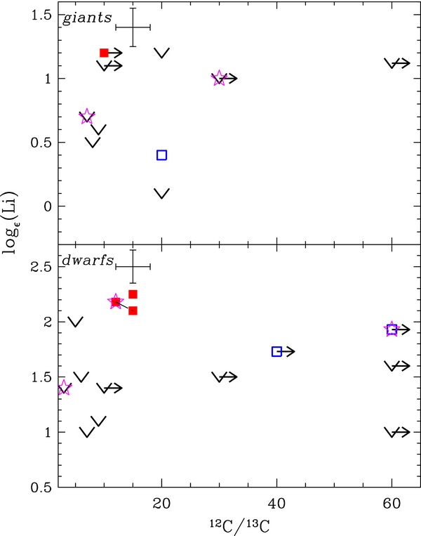
Figure 13. Lithium abundances as a function of 12C/13C ratios in CEMP "dwarfs" (lower panel) and CEMP "giants" (upper panel). Symbols are identical to Figure 10. There does not seem to be a correlation between Li depletion and 12C/13C ratio.
Download figure:
Standard image High-resolution image3.3.2. The Expected Distribution of Li Abundances
We have argued that the Li-normal CEMP stars can naturally appear in the AGB mass-transfer scenario. However, some AGB stars within a limited mass range are expected to produce Li in excess of the Spite plateau value and, if such an enriched gas is transferred to a companion, that companion should appear as a Li-rich star, unless in all cases processes in the CEMP star destroy the Li. We find no such Li-rich stars in our VLT sample, nor in the extended sample. We can test if the lack of Li-rich stars is expected in a sample of the size discussed in this paper, if AGB mass transfer is responsible for the creation of CEMP stars. As mentioned in the Introduction, the Li yields from AGB stars and the amount of mass transferred are uncertain, but we can calculate the statistics for several cases (see Table 8). In one case, we assume that the percentage of transferred mass compared to convective envelope mass is 10% (d = 0.1), similar to the ratio that Thompson et al. (2008) found for CS 22964-161. In another case, we assume that the dilution factor is so large (d = 1) that the abundances on the surface of the CEMP star reflect the yields of the AGB star for all elements. This case reflects the fact that Izzard et al. (2009) computed that as much as 0.1 M☉ should be typically accreted onto the relatively small (i.e., a few 10−3 M☉) convective envelope of the CEMP star. In contrast, we assume in the last case (d = 0.01) that the accreted material has been highly diluted into the CEMP star (possibly by thermohaline mixing; see Stancliffe et al. 2007).
Table 8. Predicted Distributions of Li Abundances
| Primary Masses | Abundance Used | Dilution | % Li-rich | % Li-normal | % Li-poor |
|---|---|---|---|---|---|
| M☉ | d | log (Li) >2.2 |
2.0 < log (Li) <2.2 |
log (Li) <2.0 | |
| 0.01 | 4 | 96 | 0 | ||
| 0.10 | 4 | 96 | 0 | ||
| 0.83 M☉–8.0 M☉ | K10 | 0.30 | 4 | 95 | 1 |
| 0.50 | 4 | 73 | 23 | ||
| 0.80 | 4 | 1 | 95 | ||
| 1.00 | 4 | 0 | 96 | ||
| 0.01 | 2 | 98 | 0 | ||
| 0.10 | 2 | 98 | 0 | ||
| 0.83 M☉–3.0 M☉ | K10 | 0.30 | 2 | 98 | 0 |
| 0.50 | 2 | 76 | 22 | ||
| 0.80 | 2 | 0 | 98 | ||
| 1.00 | 2 | 0 | 98 | ||
| 0.01 | 3 | 97 | 0 | ||
| 0.10 | 3 | 97 | 0 | ||
| 1.0 M☉–3.0 M☉ | K10 | 0.30 | 3 | 0 | 97 |
| 0.50 | 3 | 0 | 97 | ||
| 0.80 | 3 | 0 | 97 | ||
| 1.00 | 3 | 0 | 97 | ||
| 0.01 | 10 | 90 | 0 | ||
| 0.10 | 10 | 90 | 0 | ||
| 1.5 M☉–3.0 M☉ | K10 | 0.30 | 10 | 1 | 89 |
| 0.50 | 10 | 1 | 89 | ||
| 0.80 | 10 | 1 | 89 | ||
| 1.00 | 10 | 1 | 89 | ||
| 0.01 | 0 | 100 | 0 | ||
| 0.10 | 0 | 100 | 0 | ||
| 1.0 M☉–3.0 M☉ | log(Li) = −1 |
0.30 | 0 | 0 | 100 |
| 0.50 | 0 | 0 | 100 | ||
| 0.80 | 0 | 0 | 100 | ||
| 1.00 | 0 | 0 | 100 | ||
Note. K10: Li AGB yields from Karakas (2010).
Download table as: ASCIITypeset image
We use the yields of Karakas (2010), performing a linear interpolation between the model yields to predict the Li yield for stars of any mass. For AGB stars with masses less than 1.0 M☉ we adopt the ratios for a 1.0 M☉ AGB star. We also need to assume the distribution of mass ratios (q) for binaries and the range of primary and secondary masses that will produce observable CEMP stars today.
We consider several cases for the mass range of the primaries: the low-mass limit is between 0.83 M☉ and 1.5 M☉, while the high-mass limit is set to either 3 M☉ or 8 M☉. The 0.83 M☉ limit for the AGB stars at the low-mass end comes from the fact that observations of the very low mass, low-gravity star CS 30322-023 are compatible with the theoretical expectation that it is a low-mass AGB that has dredged up C, N, and s-process elements (Masseron et al. 2006). On the other hand, this low-mass limit for third dredge-up is metallicity and model dependent (e.g., Karakas et al. 2002). Depending on the assumptions in models, stars with M < 1.5 M☉ are not expected to produce enough C and s-process elements to make CEMP stars, so we adopt 1.5 M☉ as another possible limit. At the high end, the 8 M☉ limit comes from theoretical expectations of the highest mass an AGB star can have (see, for example, Ventura & D'Antona 2010). However, in AGB stars of very low metallicity (Z = 10−4 with M > 3 M☉), hot bottom burning should have occurred, which will produce nitrogen-enhanced metal-poor (NEMP) stars rather than CEMP stars.
The limits for the secondaries are always between 0.71 M☉ and 0.82 M☉, which come from demanding that the secondary star have a luminosity where its Li is not expected to be depleted (see Figure 9). We converted between luminosity and mass using a 12 Gyr Padua isochrone with Z = 0.0001 (Girardi et al. 2002). For our mass ratios, we followed the lead of Izzard et al. (2009) and adopted a flat distribution of q values, because there is no estimate in the literature of q at low metallicity. The initial Li abundance of the CEMP gas was set to 2.2; thus, any secondary with a Li abundance higher than 2.2 is labeled Li-rich.
Examination of Table 8 reveals that, regardless of the assumptions, less than 10% of dwarfs should be Li-rich if CEMP stars are the result of AGB mass transfer. In the dwarf category, we have 12 stars with a useful Li measurement, none of which are Li-rich. Therefore, our approximate calculation of the number of Li-rich stars agrees with observations. We note that any subsequent mixing in the CEMP star that destroys Li will artificially decrease the number of detected Li-rich stars, which is another reason why it is not surprising that we have not found any. The adopted yields also play a role in the expected number of Li-rich stars. According to the Ventura & D'Antona (2010) yields, for example, Li is produced in excess of the Spite plateau value for AGB stars with M > 7 M☉, which should produce substantial amounts of N and form NEMP stars rather than CEMP stars. We note that in the Galactic disk, the Li abundance in AGB stars that dredge it up from their interiors can reach very high values (log(Li) ≳ 4), but the majority of the AGB stars (∼90%) show no Li enrichment (Abia et al. 1993; Uttenthaler & Lebzelter 2010). The fact that we find no Li-rich CEMP stars may indicate that Li production during the AGB phase was rare at the metallicities of the CEMP stars, although a larger sample is necessary before any definite statement can be made.
The predicted relative numbers of Li-normal and Li-depleted stars in the absence of additional depletion in the CEMP stars depend much more on the amount of dilution than did the number of Li-rich stars. For the cases of ∼0%–20% dilution, the expected number of Li-depleted CEMP stars (i.e., log(Li) < 2.0) should be 0% and a majority of stars should be Li-normal (∼96%). The opposite is true in the case of very large dilution factors (Table 8), indicating the sensitivity of the Li abundance to details of the mass transfer rather than to AGB nucleosynthesis. We reiterate that Figures 10 and 11 show that large dilution factors should be accompanied by large C enhancements; therefore, at least some fraction of our sample of stars has likely experienced dilution factors of ∼0%–20%. More quantitatively, we can count 15 stars for which −1 < [C + N/H] < 0. This range of C+N approximately corresponds to a 10% dilution factor. Among these, 12 (∼80%) are Li-depleted. This is very far from <10% expected, based on dilution. Yet these stars are Li depleted, which must then happen during the lifetime of the CEMP star itself.
3.3.3. The Origin of the Li-depleted Stars
We have shown in Figures 10 and 11 that the low-C and low-Li stars are difficult to explain with just a dilution scenario. Therefore, some extra Li depletion should occur in the atmosphere of CEMP stars. For the case of the CEMP stars, two main physical mechanisms have been proposed in the literature that could be responsible for Li depletion: thermohaline mixing and rotation. In this section, we will examine whether either scenario is compatible with the observations of CEMP stars.
Thermohaline Mixing. Because CEMP stars have accreted large amounts of material from their companions, there are probably changes in their stellar structures that result. Whether thermohaline mixing, caused by the addition of material with a higher molecular weight on top of a material with lower molecular weight, is sufficient to explain abundance correlations in stars is still the subject of debate (Charbonnel & Zahn 2007; Eggleton et al. 2008; Denissenkov 2010; Palmerini et al. 2011), as it is dependent on the free parameter that is supposed to represent the thermohaline "finger" length. Note that while Masseron et al. (2010) did not find strong evidence for deep thermohaline mixing in CEMP stars, they could not rule it out. If it occurs, thermohaline mixing will affect other abundances besides Li. Stancliffe et al. (2009) predicted that thermohaline mixing will affect the C isotope ratios in the material transferred from the AGB star. Because of mixing in the CEMP star, the original AGB composition is not preserved, and there should be a change in the 12C/13C ratio as a function of the CEMP luminosity when the stars evolve from dwarfs to giants. If we advance the hypothesis that the observed Li-depletion spread is related to different thermohaline mixing efficiency, we would expect that the 12C/13C ratios would reflect the same efficiency. Figures 13 and 14 show no evidence to corroborate this idea. However, Stancliffe & Glebbeek (2008) noted that gravitational settling could weaken the thermohaline process. Also, Li burns at 2.5 × 10⁶ K, while CN cycling starts only at 90 × 106 K, so there is still some room for Li to be destroyed in the CEMP star while 12C/13C remains unchanged from the AGB yields. Another test is that the thermohaline strength should be correlated with the amount of accreted material, i.e., the more C is accreted on the surface of the CEMP stars, the deeper the mixing under the atmosphere of the star, and the larger the Li depletion. However, the more efficient the thermohaline mixing is, the more the accreted material is diluted. Hence, it is difficult to confidently predict an anti-correlation between C+N and Li.

Figure 14. Same as Figure 13, but for Li abundance as a function of [C/N].
Download figure:
Standard image High-resolution imageNevertheless, we stress that Stancliffe (2009) shows that thermohaline mixing inevitably leads to Li depletion, and thus the presence of Li-normal stars along Li-depleted stars with the same C+N abundances requires Li production in the AGB companion, which is uncertain (see Section 3.3.1). Although the μ-gradient established by the transfer of material should initiate thermohaline mixing in the CEMP stars' atmospheres, its efficiency and therefore its impact are difficult to detect, and it might not be the major source of the Li depletion.
Rotation. An alternative explanation for Li depletion is rotation, where the additional meridional circulation and shear turbulence drag down some Li to hotter temperatures and partially destroy it. Lithium depletion in dwarfs is not only seen in CEMP stars. Norris et al. (1997b) found three non-C-rich metal-poor stars with depleted Li. They argued that these stars were likely in binary systems that somehow caused their Li depletion. Ryan et al. (2001) and Ryan et al. (2002) further analyzed some of these Li-depleted main-sequence halo stars and presented evidence that rotation has indeed played a role in the Li destruction. Most CEMP stars are demonstrated to be old binary systems (Lucatello et al. 2005b). Indeed, increased rotational velocities of CEMP stars are all the more likely.
Figure 15 shows the Li abundances as a function of line broadening profile for the CEMP dwarfs. Broadening profiles have been derived by setting a Gaussian profile of synthetic Fe lines to match the observations. For stars that do not belong to our sample, the synthesis has been made according to the published stellar parameters and the observations have been obtained from available archives. By using this technique, the resulting broadening profile represents either the macroturbulence velocities in the atmosphere of the star, its rotation, or both (note that the broadening due to the instrument should not be a limiting factor in our case because the spectra have a resolving power high enough to resolve the intrinsic line profiles). Concerning macroturbulence broadening, 3D modeling predicts a broadening of typically 3 km s−1 for metal-poor stars (e.g., Asplund et al. 2006; Steffen et al. 2009), which is negligible compared to the broadening profiles displayed in Figure 15.

Figure 15. Lithium abundance in CEMP dwarfs as a function of rotational velocities, deduced from line broadening (symbols are the same as in Figure 10). The stars that exhibit a large broadening profile are Li depleted, while the Li-normal stars show small broadening.
Download figure:
Standard image High-resolution imageFinally, a large fraction of stars have a broadening profile >8 km s−1, which cannot be consistent with the slow rotational velocity expected for the old population of dwarfs (typically 2 km s−1; Skumanich 1972; Lucatello & Gratton 2003). Therefore, we assume that the derived velocities are mainly due to the rotation of the star, in particular for the highest values. It is notable that the largest broadening profile obtained corresponds to HE 0024-2523 (Lucatello et al. 2003), the shortest period binary known among CEMP stars, hence possibly the fastest rotating star we have considered.
In Figure 15, all stars with large rotational velocities show depleted Li. Additionally, all Li-normal stars have low rotational velocities. This indicates that rotation is responsible for depletion in some CEMP stars (at least for the fastest rotators). For this explanation to work, the degree of mixing caused by rotation needs to be large enough to destroy Li without affecting CN or carbon isotopes, because we see no correlation between [C/N] and C isotopes and rotation. However, unlike thermohaline mixing models, models of rotational mixing, at least for Sun-like stars, suggest that it destroys Li without affecting C or N until the subgiant/giant branch (Pinsonneault et al. 1989)
We note also that Li-depleted CEMP stars with low rotational velocities exist as well. Nevertheless, due to the unknown projection angle of the rotation axis of the stars, it is impossible to conclude for these stars whether the rotation is actually low in these stars or another mechanism is at work to deplete the Li. It is therefore difficult, with the current data, to exclude thermohaline mixing as the driver for Li depletion in CEMP stars. Charbonnel & Lagarde (2010) studied the complex interplay between rotation and thermohaline mixing and found that rotation favors the occurrence of thermohaline mixing in low-mass solar metallicity RGB stars. Furthermore, Stancliffe & Glebbeek (2008) show that, beyond rotation and thermohaline mixing, other mechanisms such as gravitational settling may play some role in dwarf CEMP stars and subsequently affect the observed Li abundances. In the end, the various contributions of all these physical processes may explain the observed Li abundance scatter.
3.3.4. Li in CEMP Star Subclasses
In view of the ongoing debate about whether the different CEMP subclasses are the result of the same basic phenomenon, it is interesting to compare the behavior of Li in CEMP-s, CEMP-rs, and CEMP-no stars. The last column of Table 4 reports the stellar classification as CEMP-s, CEMP-rs, or CEMP-no, for the stars of our sample based on the Ba and Eu abundances, as defined in Masseron et al. (2010). The classification for the stars mentioned in Table 7 can be found in Masseron et al. (2010). Figure 16 shows the distribution of Li abundances for stars in each subclass. There are Li-normal and Li-depleted stars in both the CEMP-s and CEMP-rs subclasses, which suggests either that the carbon for each subclass comes from a similar source or that effects in the CEMP star, such as extra mixing, dominate over the Li signature of the polluting material. All of the CEMP-no stars in the extended sample are Li depleted. The origin of CEMP-no stars is still uncertain—their peculiar abundances come either from a non-s-process-element producing AGB mass transfer or from C-rich gas coming from a previous generation of massive stars (see, e.g., Masseron et al. 2010, for more details). If the C comes from pollution by the winds of rapidly rotating massive stars, it is not clear if the Li abundances can discriminate between the scenarios, because the yields given by Meynet et al. (2006) are compatible with AGB yields down to the point that "almost no distinction could be made" (Meynet et al. 2006). Figure 10 shows that with high dilution factors (∼50%), the wind models can explain some Li-depleted CEMP-no stars with moderate carbon enhancements. The lack of Li-normal stars among the CEMP-no stars may also be the result of the combination of their metallicities and our definition of "Li-normal." Aoki et al. (2007) and Masseron et al. (2010) noted that CEMP-no stars are on average more metal-poor ([Fe/H] ≲ −2.7) than CEMP stars in other subclasses. Bonifacio et al. (2007), Aoki et al. (2009), and Sbordone et al. (2010) found that non-C-rich metal-poor stars with [Fe/H] <−3.0 appear to exhibit a decrease in Li abundance compared to the Spite plateau. Hence, the fact that we do not see Li-normal stars among CEMP-no stars might also be affected by our conservative definition of Li-normal stars, which does not encompass stars with log(Li) < 2.0. However, in the end, our sample of the CEMP-no stars is small; more Li data for this category could reveal Li-normal stars here as well.

Figure 16. Lithium abundance as a function of luminosity for different CEMP subclasses (for a detailed definition, see Masseron et al. 2010). Symbols are identical to Figure 10. The line shows our adopted separation between Li-normal and Li-depleted stars. The CEMP-s and CEMP-rs categories encompass both Li-rich and Li-depleted stars, but the CEMP-no class has only Li-depleted stars.
Download figure:
Standard image High-resolution image
The presence of Li-normal stars among CEMP-rs stars is informative for another reason. As observed by Masseron et al. (2010), some CEMP stars, mostly in the CEMP-rs subclass, lie off the standard evolutionary tracks and are more luminous or bluer than expected from isochrones of the appropriate metallicities. It is not yet clear why these stars show such properties, but some of the scenarios for forming field blue stragglers imply mass transfer of material, as is the case for CEMP-rs stars. CEMP-rs stars show the highest enhancements of C and neutron-capture elements in their atmospheres. This could drive efficient thermohaline mixing, which drags the C-enriched material down to the core and boosts the luminosity of the stars through the CNO cycle (Stancliffe et al. 2007). In any possible scenarios, Li should have been heavily destroyed. However, the upper panel of Figure 16 shows that there are Li-normal stars in the CEMP-rs class. Therefore, the reason why some CEMP-rs stars are not located on the regular track of the H-R diagram remains unsolved.
4. CONCLUSIONS
We have used Li abundances and carbon isotope ratios to test the origin of carbon and the presence of mixing and dilution in CEMP stars. We observe a large range of Li abundances in CEMP stars. If moderate amounts of AGB material are transferred to the CEMP star, then dilution appears to explain Li-normal stars. Although we cannot completely rule out that some Li may have been produced in a former AGB companion, it is definitely not required to invoke that process to explain the CEMP stars with Li abundances close to the Spite plateau value. In contrast, it appears difficult to explain the CEMP stars where the Li is depleted without additional Li depletion in the CEMP star itself. Hence, extra mixing is required. Although thermohaline mixing is indeed an obvious candidate to explain Li depletion in some CEMP stars, we did not find any correlation between the CEMP properties extensively explored by Stancliffe (2009) and Li depletion. However, rotation seems to play a prominent role for some CEMP stars. We predict that the fastest rotating stars (which correspond to the stars with the largest broadening profiles) should exhibit the largest Li depletion. This result is in line with the recent findings of Smiljanic et al. (2010) and Canto Martins et al. (2011), showing that the inclusion of rotation in the evolutionary models can reproduce Li depletion in open clusters.
Because the current sample of CEMP stars with Li measurements is still small, we could not definitively infer a dependency of the rotational velocity on the amount of Li depletion. Larger samples and more systematic radial velocity monitoring are required to confirm these results.
We thank T. Dermine for discussions on binary accretion and N. Behahra for providing spectra. We acknowledge support from NSF AST-0607482 and AST-0707948. T.C.B. acknowledges partial support from grants PHY 02-16783 and PHY 08-22648: Physics Frontiers Center/Joint Institute for Nuclear Astrophysics (JINA), awarded by the U.S. National Science Foundation. N.C. acknowledges support by Sonderforschungsbereich SFB 881 "The Milky Way System" (subproject A4) of the German Research Foundation (DFG).
Footnotes
- *
Based on observations collected at the European Southern Observatory, Paranal, Chile (Proposal Number 076.D-0451A).