


ABSTRACT
With the development of one-dimensional stellar evolution codes including rotation and the increasing number of observational data for stars of various evolutionary stages, it becomes more and more possible to follow the evolution of the rotation profile and angular momentum distribution in stars. In this context, understanding the interplay between rotation and convection in the very extended envelopes of giant stars is very important considering that all low- and intermediate-mass stars become red giants after the central hydrogen burning phase. In this paper, we analyze the interplay between rotation and convection in the envelope of red giant stars using three-dimensional numerical experiments. We make use of the Anelastic Spherical Harmonics code to simulate the inner 50% of the envelope of a low-mass star on the red giant branch. We discuss the organization and dynamics of convection, and put a special emphasis on the distribution of angular momentum in such a rotating extended envelope. To do so, we explore two directions of the parameter space, namely, the bulk rotation rate and the Reynolds number with a series of four simulations. We find that turbulent convection in red giant stars is dynamically rich, and that it is particularly sensitive to the rotation rate of the star. Reynolds stresses and meridional circulation establish various differential rotation profiles (either cylindrical or shellular) depending on the convective Rossby number of the simulations, but they all agree that the radial shear is large. Temperature fluctuations are found to be large and in the slowly rotating cases, a dominant ℓ = 1 temperature dipole influences the convective motions. Both baroclinic effects and turbulent advection are strong in all cases and mostly oppose one another.
Export citation and abstract BibTeX RIS
1. OBSERVATIONS AND MODELS OF RGB STARS
1.1. What are Observations and Stellar Evolution Models Telling Us?
Almost all, if not all stars rotate, and the distribution of their angular momentum appears to change along the course of their evolution as can be seen from the υ sin i data collected during the last decades for stars all over the HR diagram (e.g., see for instance Pilachowski & Milkey 1984, 1987; de Medeiros & Mayor 1999; Glebocki & Stawikowski 2000; Royer et al. 2002a, 2002b; Barnes et al. 2005; Karl et al. 2005; Carney et al. 2008).
To constrain the internal angular momentum profile at each evolutionary phase, the easiest approach would be to probe stellar interiors in order to derive the angular velocity profile. Helioseismology allows us to invert the inner solar rotation profile down to r = 0.25R☉ (Schou et al. 1998; Antia & Basu 2000; Antia et al. 2008; García et al. 2008). Asteroseismology should soon offer similar opportunities for other stellar spectral types thanks to the CoROT (Goupil et al. 2006; Baglin et al. 2007) and Kepler satellites. In the meantime, however, we are left with indirect probes of the internal angular momentum distribution in all stars: (1) the surface velocity measurements for stars of similar initial mass at different evolutionary stages; (2) the surface abundance anomalies resulting from the action of internal transport processes, in part due to rotation, that connect the stellar envelopes to the nuclearly processed internal regions. These indirect probes can be compared to the results of one-dimensional rotating stellar evolution models (Pinsonneault et al. 1989; Fliegner & Langer 1994; Meynet & Maeder 1997; Talon et al. 1997; Maeder & Meynet 2000; Heger et al. 2000, 2005; Palacios et al. 2003, 2006; Chanamé et al. 2005; Suijs et al. 2008) in order to guess the angular velocity profile evolution. The introduction of rotation and associated transport processes in one-dimensional stellar evolution models leads indeed to a clear improvement of the comparison between theoretical predictions and observations, in particular from the point of view of chemical abundances. However, a number of points, in particular concerning the evolution of the surface rotation velocities, remain to be elucidated. It is the case for the differences between predicted and observed spin rates for white dwarfs and neutron stars (Heger et al. 2005; Suijs et al. 2008), or the interpretation of the surface velocities distribution of horizontal branch stars (Sills & Pinsonneault 2000; Recio-Blanco et al. 2002, 2004).
While important theoretical developments have been devoted to the description of the one-dimensional angular momentum transport in the radiative stellar interiors (Zahn 1992; Maeder & Zahn 1998; Mathis & Zahn 2004), the transport of angular momentum in convective regions, and in particular in extended convective envelopes, is poorly described in one-dimensional models. This is of particular importance for the case of giant stars that possess very extended convective envelopes, occupying up to 80% and more of the total stellar radius. These stars are expected to have very slow surface rotation due to their large radius, which is confirmed by observations (de Medeiros & Mayor 1999; Carney et al. 2008), but may also have a rapidly rotating core (Sills & Pinsonneault 2000).
Understanding the angular momentum distribution during the giant evolutionary phases is crucial to understand the subsequent evolutionary phases, and the spin rates of compact stellar remnants. It relies on the understanding of the interplay between convection and rotation in these very large convective envelopes. Few observational constraints are available though, due to the difficulty to measure rotation velocities for cool and slowly rotating stars exhibiting broadened spectral lines. For the case of active giants exhibiting spots at their surface, we may mention the possibility to reconstruct their latitudinal surface rotation from spectropolarimetric data (Petit et al. 2002). These type of data are however limited, and three-dimensional numerical experiments appear to be the best start to ascertain the behavior of rotating extended convective envelopes of red giant stars.
1.2. Present Status of Three-dimensional Simulations
The study of turbulent convection in rotating media requires global three-dimensional simulations of convection in spherical geometry, which is both computationally very demanding and difficult to achieve due to the large number of scales that have to be represented. It is only in the last two decades that such an approach was made possible, in particular thanks to the development of massively parallel computer architectures. Most of the simulations of convection in astrophysics have been obtained in the context of the Sun (e.g., Stein & Nordlund 1998; Brun & Toomre 2002; Miesch et al. 2006, 2008), and led to a great improvement of our understanding of the solar convection. Concerning the convection realized in extended envelopes of red giant stars, three-dimensional hydrodynamical simulations of the convection in a red supergiant star (Freytag et al. 2002, hereafter FSD02; "star-in-a-box" experiment) and in asymptotic giant branch (AGB) stars (e.g., FSD02; Woodward et al. 2003, hereafter WPJ03) have been performed using fully compressible codes. These simulations do not include rotation and present as a common feature of the development of pulsations without any κ-mechanism. In the AGB star by WPJ02, the convective pattern appears to have a dipolar nature, which is also found by Kuhlen et al. (2006) in their simulation of nonrotating fully convective spheres in carbon–oxygen white dwarfs, and by Steffen & Freytag (2007, hereafter SF07) in their nonrotating "star-in-a-box" mini-sun experiment. In the FSD02 simulations of both the red supergaint and the AGB star, the convective pattern achieved consists in a small number of large cells covering the surface, the number of which increases with resolution. The surface patterns obtained by WPJ03 in their higher resolution simulations are more complex, yet resembling that found by FSD02: large warm upgoing flows surrounded by narrow cooler downgoing structures.
Recently, SF07 presented rotating "star-in-a-box" experiments. They find no striking difference in the convective pattern compared to their nonrotating case. Concerning rotation, they find a strong differential rotation, which is anti-solar in latitude, and very strong meridional circulation flows, comparable to typical convective velocities.
Other three-dimensional simulations of the convection in the upper envelope and the atmosphere of red giants have been performed in a more local approach, within the framework of realistic simulation of spectral lines formation in these stars (e.g., Chiavassa et al. 2006; Collet et al. 2007; Robinson et al. 2004). In these works, the hydrodynamical simulation of convection itself is not discussed in details. Let us finally mention the work by Herwig et al. (2007), who investigated the convection in the thermal pulses of an AGB star.
In order to further study the heat, energy, and angular momentum redistribution occurring in the extended convective envelope of slowly rotating red giant branch (RGB) stars, we have started a series of three-dimensional hydrodynamical simulations with the Anelastic Spherical Harmonics (ASH) code (Palacios & Brun 2007). In the present paper, we explore the parameter space by varying the rotation rate and the turbulence level of our RGB models and discuss in length the dynamics of such complex systems. More specifically, in Section 2 we describe our numerical approach and the three-dimensional ASH code as well as specify the one-dimensional stellar evolution model used to set our background reference state. Then, in Section 3 we discuss the properties of the turbulent convection achieved in our simulations. Large-scale flows are discussed in Section 4, with a particular emphasis on the internal rotation profile. We finally analyze and describe in Section 5 the transport of heat and angular momentum in our simulations, before summarizing the overall results and concluding in Section 6.
2. EQUATIONS, BOUNDARY CONDITIONS, AND PARAMETER VALUES
2.1. Anelastic Equations
The simulations described here were performed using our ASH code. ASH solves the three-dimensional anelastic equations of motion in a rotating spherical geometry using a pseudospectral semi-implicit approach (e.g., Clune et al. 1999; Miesch et al. 2000; Brun et al. 2004). These equations are fully nonlinear in velocity variables and linearized in thermodynamic variables with respect to a spherically symmetric mean state. This mean state is taken to have density  , pressure
  , temperature
  , specific entropy
  ; perturbations about this mean state are written as ρ, P, T, and S. Conservation of mass, momentum, and energy in the rotating reference frame are therefore written as

where cp is the specific heat at constant pressure, v = (vr, vθ, vϕ) is the local velocity in spherical geometry in the rotating frame of constant angular velocity  , g is the gravitational acceleration, κr is the radiative diffusivity, and
  is the viscous stress tensor, with components

where eij is the strain rate tensor. Here, ν and κ are effective eddy diffusivities for vorticity and entropy. To close the set of equations, linearized relations for the thermodynamic fluctuations are taken as
assuming the ideal gas law
where  is the gas constant. The effects of compressibility on the convection are taken into account by means of the anelastic approximation, which filters out sound waves that would otherwise severely limit the time steps allowed by the simulation.
For boundary conditions at the top and bottom of the domain, we impose
- 1.impenetrable walls:

- 2.stress free conditions:
- 3.and constant entropy gradient:
Convection in stellar environments occurs over a large range of scales. Numerical simulations cannot, with present computing technology, consider all these scales simultaneously. We therefore seek to resolve the largest scales of the nonlinear flow, which we think are likely to be the dominant players in establishing differential rotation and other mean properties in convective envelopes. We do so within a large-eddy simulation (LES) formulation, which explicitly follows larger scale flows while employing subgrid-scale (SGS) descriptions for the effects of the unresolved motions. Here, those unresolved motions are treated as enhancements to the viscosity and thermal diffusivity (ν and κ), which are thus effective eddy viscosities and diffusivities. For simplicity, we have taken these to be functions of radius alone, and to scale as the inverse of the square root of the mean density. We emphasize that currently tractable simulations are still many orders of magnitude away in parameter space from the highly turbulent conditions likely to be found in real stellar convection zones. These LESs should therefore be viewed only as indicators of the properties of the real flows. We are however encouraged by the success that similar simulations (e.g., Miesch et al. 2000; Elliott et al. 2000; Brun & Toomre 2002; Miesch et al. 2006) have enjoyed in matching the detailed observational constraints for the differential rotation within the solar convection zone provided by helioseismology.
2.2. Brief Summary of the Numerical Method
Thermodynamic variables within ASH are expanded in spherical harmonics Ymℓ(θ, ϕ) in the horizontal directions and in Chebyshev polynomials Tn(r) in the radial direction. Spatial resolution is thus uniform everywhere on a sphere when a complete set of spherical harmonics of degree ℓ is used, retaining all azimuthal orders m. We truncate our expansion at degree ℓ = ℓmax, which is related to the number of latitudinal mesh points Nθ (here ℓmax = (2Nθ − 1)/3), take Nϕ = 2Nθ azimuthal mesh points, and utilize Nr collocation points for the projection onto the Chebyshev polynomials. We have considered various grid resolutions Nr × Nθ × Nϕ depending on the degree of turbulence of the model (see Table 1). A semi-implicit, second-order Crank-Nicolson scheme is used in determining the time evolution of the linear terms, whereas an explicit second-order Adams-Bashforth scheme is employed for the advective and Coriolis terms. The ASH code has been optimized to run efficiently on massively parallel supercomputers such as the IBM SP-6 or SGI Altix, and has demonstrated excellent scalability on such machines (see Clune et al. 1999 and Brun et al. 2004 for more details).
Table 1. Parameters for the Four Simulations
| Case | RG1 | RG1t | RG2 | RG2t |
|---|---|---|---|---|
| Nr, Nθ, Nϕ | 257, 256, 512 | 257, 512, 1024 | 257, 256, 512 | 257, 768, 1536 |
| Ra ... | 8.25 × 10⁵ | 3.18 × 10⁶ | 7.45 ×10⁵ | 2.69 × 10⁶ |
| Ta ... | 1.32 × 10⁶ | 4.89 × 10⁶ | 5.44 × 10⁴ | 1.96 × 10⁵ |
| Pr ... | 1 | 1 | 1 | 1 |
| Roc ... | 0.791 | 0.806 | 3.703 | 3.703 |
| νtop ... | 1.2 × 10¹⁵ | 5 × 10¹⁴ | 1.2 × 10¹⁵ | 5 × 10¹⁴ |
| κtop ... | 1.2 × 10¹⁵ | 5 ×10¹⁴ | 1.2 × 10¹⁵ | 5 × 10¹⁴ |
 ... ... |
256 | 623 | 372 | 882 |
 ... ... |
256 | 623 | 372 | 882 |
 ... ... |
0.281 | 0.284 | 2.03 | 2.01 |
Notes. All simulations have an inner radius rbot = 1.36 × 1011 cm, an outer radius rtop = 1.36 × 1012 cm, with L = 1.22 × 1012 cm (≃17.6 R☉). The number of radial, latitudinal, and longitudinal mesh points are Nr, Nθ, and Nϕ, respectively. The higher degree of turbulence in cases RG1t and RG2t was obtained by maintaining the Prandtl number at 1 and lowering both the eddy viscosity ν and eddy diffusivity κ at the top edge of the domain. ν and κ are given in units of cm s−2. The characteristic numbers evaluated at mid-layer depth are the Rayleigh number Ra = (∂ρ/∂S)ΔSgL3/ρνκ, the Taylor number Ta = 4Ω20L4/ν2, the Prandtl number Pr = ν/κ, the convective Rossby number  , the rms Reynolds number
  , the rms Péclet nulber
  , and the rms Rossby number
  . We use the rms convective velocity
  at mid-depth given in Table 2 to compute these quantities and the following mid-depth viscosity of 8.481014 (3.531014) cm s−2 for, respectively, the laminar (turbulent) cases.
Download table as: ASCIITypeset image
2.3. Computing a RGB Star with ASH
The models considered here are intended to be simplified descriptions of the bulk of the deep extended convective envelope of an evolved (RGB phase) 0.8 M☉ star. We do not consider in this study the presence of an overshooting layer (compare Miesch et al. 2000; Browning et al. 2006; Brun 2009). Contact is made with a one-dimensional stellar model (at an age of 11 Gyr) for the initial conditions, which adopts realistic values for the radiative opacity, density, and temperature Palacios et al. (2006). This one-dimensional model was computed with the STAREVOL stellar evolution code (see Siess et al. (2000) and Siess (2006) for more details on the numerical methods and physical ingredients adopted). Convection is computed within STAREVOL using a classical mixing length treatment with a parameter αMLT = 1.75, and the convective limits are determined according to the Schwarzschild criterion for the convective instability. The luminosity of the modeled star L* is 425 L☉, its radius R* is about 40 R☉. Our simplified three-dimensional simulations were initialized using the radial profiles of gravity g, radiative diffusivity κrad, and the mean density  of the one-dimensional model along with a prescribed mean entropy gradient
  as the starting points for an iterative Newton–Raphson solution for the hydrostatic balance and for the gradients of the thermodynamic variables. The mean temperature
  is then deduced from Equation (6). This technique yields background reference profiles in reasonable agreement with the thermally relaxed one-dimensional stellar model as can be seen in Figure 1, and we are thus confident that the background state of our simulations is close to their final relaxed state. We have built four different models that all share this one-dimensional structure, and list their most important parameters in Table 1. Cases RG1 and RG1t are computed with an initial bulk rotation rate Ω0 = Ω☉/10 = 2.6 × 10⁻⁷ rad s−1 (or a rotation period Prot of ∼280 days), while we have used Ω0 = Ω☉/50 = 5.2 × 10⁻⁸ rad s−1 (or Prot∼1400 days) for cases RG2 and RG2t. Cases RG1t and RG2t are more turbulent versions of cases RG1 and RG2, respectively (that have been published in Palacios & Brun 2007). Case RG2 has been evolved from scratch, but we have also checked that reducing the rotation rate of case RG1 down to the value adopted for case RG2 leads to the same configuration in terms of convection and rotation. For this reason, cases RG1t and RG2t have been, respectively, evolved from cases RG1 and RG2 by progressively reducing the effective values of κtop and νtop.
Figure 1. Profiles of the temperature, density, pressure, and convective velocity as a function of the radius in the one-dimensional model (solid lines) that were used as a background for the three-dimensional simulations, and the actual profiles used in the ASH simulations (dashed lines). The hatched regions show the computational domain considered in the three-dimensional model.
Download figure:
Standard image High-resolution imageAlthough the large rotation adopted for cases RG1 (and RG1t) corresponds to a surface equatorial velocity much larger than that inferred from observations, these two cases could be viewed as less evolved counterparts of cases RG2 and RG2t, respectively, since the surface rotation will decrease as the radius increases during the ascent of the RGB due to angular momentum conservation.4
All the models presented here have been computed over several rotation periods and about one hundred convective overturning times (or about 20–30 years of physical temporal evolution). This long temporal evolution is required in order to reach a statistically stationary state and equilibrated balances of energy, heat, and angular momentum within the convective shell. Even though the Kelvin–Helmotz time τKH ∼ GM2*/R*L* is about 1200 years for our RGB models, we believe that the properties of the models discussed in the subsequent sections correspond to a mature and well equilibrated state. Of course, we cannot rule out a very slow evolution of the model when integrated over "very long period of time" (as done in Chan 2007), but given the realistic one-dimensional structure used for the background state and the small Mach number (i.e., small temperature and density fluctuations with respect to the mean background values) realized in our simulations we are convinced that our results are robust and a fair description of the nonlinear dynamics present inside a rotating convective envelope. In order to reach such an equilibrated state, we have use a large amount of CPU-time on massively parallel computers (of order 600,000 hr and more per simulation), in particular with cases RG2 and RG2t, due to their long rotation period.
Given reasonable computing resources, the ASH code does not allow at present to compute the full convective envelope of a RGB star, in which the density varies by more than 4 orders of magnitude, but only a portion of it (see Figure 1). We will thus assume in all the cases presented in this paper a density variation of 2 orders of magnitude. This choice translates into computing the inner half (e.g., from rbot = 0.05 R* up to rtop = 0.5 R*) of the extended convective envelope of a 0.8 M☉ RGB star. We concentrate on the inner part of the convective envelope, since near the surface the Mach number would be too large for the anelastic formalism to remain valid. Moreover, this deeper part of the extended convective envelope is particularly interesting from the point of view of one-dimensional stellar evolution models, because it is the region that may gradually be incorporated into the underlying radiative zone, and thus establish the link between nuclearly processed regions and the chemically homogeneous convective envelope. Indeed, during the RGB ascent, the angular momentum of the innermost part of the convective envelope will be transferred to the underlying radiative interior as the convective envelope retreats in mass after the first dredge-up Clayton (1968). This will influence the rotation-induced transport of both angular momentum and chemicals in the radiative zone.
3. PROPERTIES OF TURBULENT CONVECTION IN THREE-DIMENSIONAL RGB STAR MODELS
The convective envelope occupies more than 80% of the stellar radius in red giants, thus making the understanding of the physical processes acting in this region very important in order to get a complete description of these stars. The turbulent convection in the outer envelope of giants is expected to be large scale and time dependent from nonrotating simulations (FDS02). In this section, we will start by describing in details the convective patterns achieved in our simulations and their temporal evolution.
Figure 2 presents for case RG1t the temporal evolution of the volume averaged total kinetic energy density and of its components split into differential rotation kinetic energy (DRKE), meridional circulation kinetic energy (MCKE), and nonaxisymmetric convective kinetic energy (CKE; see Brun & Toomre 2002 for their analytical expression). By assuming an initial negative mean entropy gradient  and a supercritical Rayleigh number, we trigger the development of the convective instability from the quiescent state by introducing in the model three-dimensional random perturbations of the entropy and velocity fields. After a phase of exponential growth of the convective instability lasting less than 200 days, the simulation reaches a nonlinear saturation phase after 300 days, leading to a statistically stationary state of the convective motions over more than ten rotation periods (several thousands of days). This behavior is found in all of our four cases but RG1 and RG1t possess a more stable long-term behavior (see below). In the example presented in Figure 2 for RG1t, the kinetic energy in convective motions dominates the energy in differential rotation and that in meridional flows (CKE > DRKE > MCKE). This hierarchy is maintained ever since the simulation reaches the statistically stationary state in both models RG1 and RG1t. In models RG2 and RG2t, due to their slower rotation, the kinetic energy distribution is different as will be discussed in more details together with cases RG1 and RG1t in Section 5.1.
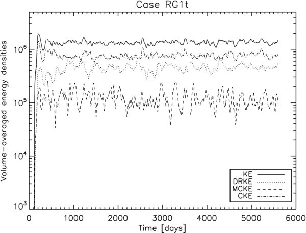
Figure 2. Temporal evolution of the volume averaged total kinetic energy density (KE) and of its components from convection (CKE), differential rotation (DRKE), and meridional circulation (MKE) for case RG1t.
Download figure:
Standard image High-resolution imageOnce the stationary state realized, the radial energy flux balance reaches equilibrium (i.e., energy input = energy output =L*) as can be seen in Figure 3. This figure represents the radial transport of energy in case RG1t achieved by the radiative flux Fr, the enthalpy flux Fe, the kinetic energy flux Fk, the viscous flux Fν, and the unresolved flux Fu, all converted to luminosity and normalized to the stellar luminosity L*. We note that the enthalpy flux is dominant over most of the domain and reaches values (when converted to luminosity) representing 140% of the total stellar luminosity. This very large flux arises to compensate the inward directed (negative) kinetic energy flux. At the domain's bottom and top edges, the diffusive flux (radiative and unresolved) carry the energy. The viscous flux is negligible. As already mentioned in Palacios & Brun (2007), the strong inward directed kinetic energy flux found in this simulation is in contradiction with one of the basic hypothesis of the Mixing Length Theory (MLT) used in most of one-dimensional stellar evolution codes to model convection, e.g., that Lconv ≡ Le = L*. This result has also been found by WPJ03 in their three-dimensional simulation of the convective envelope of a 3 M☉ AGB star. In a forthcoming paper, we plan to test a more realistic formulation of the MLT in one-dimensional stellar evolution models based on the results of the present study.

Figure 3. Energy flux balance as a function of radius, averaged over horizontal surfaces and in time over the last 10 rotation periods for case RG1t. The net flux is separated into five components: enthalpy flux Fe, radiative flux Fr, unresolved eddy Fu, kinetic energy flux Fk, and viscous flux Fv. The fluxes and radius are normalized with respect to the stellar luminosity and radius, respectively.
Download figure:
Standard image High-resolution image3.1. Organization of Convection
The strong radial enthalpy flux found in our simulations results from the correlation between radial velocity and temperature fluctuations shown for RG1t in Figure 4 (left and middle panels), where we display horizontal maps of vr and T (and enstrophy).
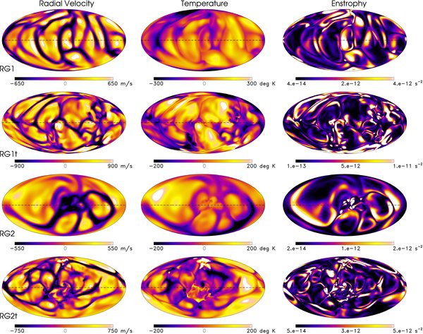
Figure 4. Convection at the top edge of the computational domain of case RG1 after 3845 days (first row), case RG1t after 4637 days (second row), case RG2 after 7212 days (third row), and case RG2t (forth row) 6353 days. The radial velocity, temperature, and enstrophy are represented at r = 19 R☉.
Download figure:
Standard image High-resolution imageThe convective patterns realized in our four models vary significantly depending on the adopted reference rotation frame Ω0. Cases RG1 and RG1t rotating at one tenth the solar rate possess about 10 downflow lanes over the uppermost layers. These relatively cool downflow lanes are interconnected, forming an intricate network surrounding warm broad upflows. They appear respectively in blue (cool downflows) and reddish (warm upflows) in Figure 5, where we present a three-dimensional rendering of the temperature and velocity in the model RG1t. They present some systematic alignment with the north–south direction, such property being quite obvious for the least turbulent case RG1. Large velocity and temperature fluctuations are observed throughout the domain (as also evident in Figure 8 for the velocity where we plot the radial profile of the rms velocity components), a direct consequence of the high luminosity of the modeled star. Typical values for these quantities are ±300 K and ±1000 m s−1 in most of the computational domain, in keeping with the necessity of convection to carry outward the large imposed radiative flux. Comparatively to the simulations of the solar convection envelope, these values are at least 1 order of magnitude larger (Brun & Toomre 2002). The patterns described for the velocity fluctuations are also visible in the temperature fluctuations. The contrast between hotter and cooler parts is however weaker than that existing between upflows and downflows in the velocity maps. Nonetheless, due to our choice of a Prandtl number Pr = 1, they exhibit the same fine structures. Those structures are particularly obvious in the enstrophy map (right panel of Figure 4), with downflow lanes being part of an intricate network and possessing the highest enstrophy concentration near the interstices. This is a direct consequence of the fact that as flows converge toward the downdraft they acquire intense cyclonicity, whereas upflows expand as they rise and lose their cyclonic character. The vortex tubes seen in the enstrophy map actually come by pair of opposite gyres. They are the weaker and broader equivalent to the intense "cold spinners," seen in solar convection simulations (Miesch et al. 2008). In Figure 6, we plot the radial vorticity map at the same radius as in Figure 4 for cases RG1t and RG2t. For case RG1t, the radial vorticity presents near the top of the domain a clear dominant negative (positive) value in the northern (southern) hemisphere, respectively, a direct consequence of the action of the stronger Coriolis force in this more rapidly rotating model.
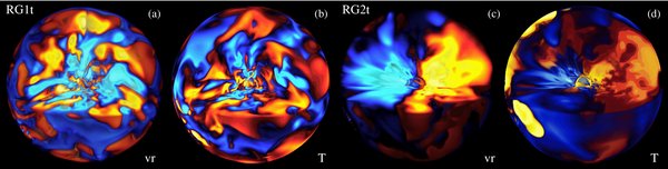
Figure 5. Three-dimensional rendering of the convective radial velocity (a, c) and of the temperature (b, d) in our simulations RG1t and RG2t. In panels (a, b), a global view from which we have extracted an octant is shown. We can thus see the equatorial and meridional planes and have a sense of the flow convergence. In panels (c, d), a global view from which we have extracted a quadrant is shown. This helps seeing the dipolar nature of the convection. In all panels, the blue (red) parts correspond to downward (upward) flows and cool (warm) temperature fluctuations. The three-dimensional rendering has been done with the SDvision software (Pomarede et al. 2008).
Download figure:
Standard image High-resolution image
Figure 6. Radial vorticity maps for cases RG1t and RG2t represented at r = 19 R☉, after 4637 and 6353 days, respectively.
Download figure:
Standard image High-resolution imageTurning to the slowly rotating cases RG2 and RG2t in Figure 4, we clearly note a pattern change. This is mostly due to a weaker influence of rotation on convection (as illustrated in Table 1 by their larger convective Rossby number with respect to cases RG1 and RG1t) leading to more vigorous and isotropic flow. The downflow lanes show much less systematic alignment with respect to the north–south direction. The weaker influence of rotation also leads to a shift toward a smaller number of downflow lanes over the surface, with here only between 4 and 6 lanes covering the top of the computational domain. Further a strong dipole in temperature is observed, with two separate large regions of the surface being respectively predominantly cool and warm (cf. Section 5.1 for more details). As a consequence of this thermal structuration of the convective flow, a large coherent circulation sets in between these two regions, yielding two zones that are respectively filled mostly with converging narrow downflows on the one hand and diverging broad upflows on the other hand. This dipole in temperature and velocity persists in depth as can be seen from the equatorial slices presented in Figure 7 for case RG2t. We clearly note the large inflow in the top part of the figure with the corresponding outflow on the other side of the central region. This large-scale flow goes through the central part without any difficulty connecting efficiently regions of the domain that are far apart. The temperature patterns are more finely structured but overall there is good correlation between respectively the cold (warm) and inflow (upflow) regions. This bipolar structure of convection is a very interesting property of our slowly rotating case and points toward the results previously obtained by Porter & Woodward (2000), WPJ03, and SF07 in nonrotating hydrodynamical simulations. Indeed these authors report in their nonrotating giant stars the presence of dominant large-scale convective cells over the star's top domain embedded in a dipolar flow crossing the whole convection domain. It is interesting to note that Chandrasekhar (1961) in his linear axisymmetric study of the onset of convection in a spherical shell, has demonstrated that the ℓ = 1 mode is for small aspect ratio, one of the most unstable modes to excite. This is mostly due to a geometrical effect with convection rolls having more space to develop for low-aspect ratio (or full sphere) than for large-aspect ratio (thin shell), thus leading to larger physical structures and favoring the low ℓ modes. We have also run a nonrotating simulation for the very same initial structure as that used for the four cases discussed in the present paper, and this dipolar structure also shows up clearly in that simulation (which is not presented here). This dipole can only be guessed in the three-dimensional equatorial cut presented in Figure 5 for model RG1t.

Figure 7. Equatorial slices for the radial velocity and the temperature in model RG2t. The bipolar structure of the convective flow appears clearly in both maps. The dotted, dashed, and dashed-dotted circles indicate the depths at R = 19 R☉, 11 R☉, and 3 R☉, respectively, also used in Figures.
Download figure:
Standard image High-resolution imageAs for cases RG1 and RG1t, the more slowly rotating models possess some enstrophy, with the downflows having the largest values due to their cyclonic character. The radial vorticity map for case RG2t shown in Figure 6 does not possess a dominant sign per hemisphere, contrary to case RG1t even though there seems to be some weak tendency for a negative/positive orientation (sign) to dominate near respectively the warm/cool regions. The less systematic orientation in each hemisphere of the radial vorticity, again, is a consequence of the larger convective Rossby number of this slowly rotating model, and of the weaker hemispherical anisotropy imposed by the Coriolis force of the flows.
We display on Figure 8 the radial profile of the total rms velocity and its radial, latitudinal and longitudinal components for cases RG1, RG1t, RG2, and RG2t. Typical values are of 1–3 km s−1 to be compared with a sound speed evolving in the range 25–80 km s−1 in the models, thus a posteriori confirming the validity of the anelastic approximation (see also Figure 1). We note that the radial velocity dominates in the bulk of the computational domain roughly between r = 0.07 R* and r = 0.3 R*. This is due to the continuous acceleration of the convective plumes over the whole domain depth, with  becoming maximal near the bottom. In the more slowly rotating cases RG2 and RG2t,
  is even faster due again to the reduced influence of rotation on the vigor of the convective motions and possess a pronounced bell-like profile. It is indeed known since (Chandrasekhar 1961) that rotation tends to inhibit convection by increasing the critical Rayleigh number, thus leading to a decrease of the supercriticality of the models for a given Ra. Due to our rigid (impenetrable) boundary conditions, the radial velocity is forced to vanish at the domain's edges explaining its peculiar shape. Independent of the adopted Reynolds number, the horizontal rms velocity components have very similar amplitudes.
  profiles slightly differ between the slow and faster models, with the slower models having a steeper profile in the outer parts of the computational domain. This is due to the shellular rotation existing in the slowly rotating models as will be discussed in the following sections. In all our four cases, the horizontal components dominate toward the top of domain. At the bottom boundary, the horizontal flow amplitudes increase significantly possibly due to local angular momentum conservation as the flow converge toward the center. This is even more evident for cases RG2 and RG2t, where the inner shells have much faster horizontal velocities due to the shellular rotation.

Figure 8. Profiles of the rms radial ( : dashed), latitudinal (
 : dotted dashed), longitudinal (
 : dotted), and total (
 : solid) velocities in the computational domain obtained for cases RG1, RG1t, RG2, and RG2t after 12, 6, 10, and 1/2 rotation periods, respectively. Also plotted is the rms temperature profile (cross symbols) with the corresponding scale given on the right y-axis.
Download figure:
Standard image High-resolution image3.2. Temporal Evolution of Convective Patterns
The temporal evolution of the convective patterns for case RG1t is shown in Figure 9, which displays four sequences of images of the radial velocity at three different depths over a period of about 96 days. The first row shows the equatorial plane at each timeshot, and the different depths represented in Mollweide projections are indicated with dotted, dashed, and dashed-dotted black circles for 19 R☉ (second row), 11 R☉ (third row), and 3 R☉ (forth row), respectively. As can be seen from the equatorial cuts and the first row of Mollweide projections at 19 R☉, the convective structures at the top of the computational domain move from east to west (retrograde, i.e., clockwise). Deeper in the convective region, structures have a prograde (counterclockwise) displacement. The equatorial cuts indicate that the up and downflows maintain their coherence over most of the computational domain. This is far less evident from the Mollweide projections due to the large geometrical factor between both edges of the domain, as well as to the intrinsic tilt of the structures.
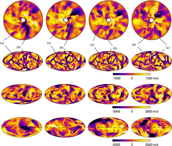
Figure 9. Evolution of the convection over 96 days in case RG1t. The first row displays the radial velocity in equatorial slices at the four time steps selected. The dotted (dashed, dashed-dotted) black ring indicates the depth r = 19 R☉ (r = 11 R☉, r = 3 R☉), at which the projection shown in the second (third, fourth) row is drawn. The time interval between each successive image is about 24 days (the global rotation rate of case RG1t is a tenth the solar value). The color coding adopted for the equatorial slices is the same as that used at r = 11 R☉ (third row). The black lines indicate the correspondence of the patterns between the equatorial and Mollweide representations.
Download figure:
Standard image High-resolution imageThe evolution presented here corresponds to about a third of the rotation period of case RG1t (see Table 1). The global convective overturn given by
is of 75 days in this case, which is much shorter than the rotation period. For this reason, we completely lose track of the structures when considering a complete rotation. This is also the case for our model RG1. For the slowly rotating cases RG2 and RG2t, this is even more striking, since the convective overturn is again of about 80 days, while the rotation period is 1398 days.
4. ASSOCIATED LARGE-SCALE FLOWS
As we have seen above, the influence of rotation on convection is strong and leads to significant change in the overall dynamics of our extended convective envelope. It is of fundamental interest to assess how such convection zone redistributes angular momentum, energy, and heat leading to large-scale horizontal flows such as differential rotation or meridional circulation. It has also a potential impact on how these stars evolve on the giant branch and process nuclides in their radiative interior. In this section, we report on the various profiles achieved by our four models deferring to Section 5 the detailed analysis of their physical origin.
4.1. Internal Rotation Profile
As discussed in the introduction, the rotation profile established in the convective envelope of RGB stars is particularly important to the understanding of their global evolution. We believe that our models can give us a good hint of such profiles as a function of depth and latitude.
In Figure 10, we display contours of the longitudinal and temporal average of the angular velocity realized in our four models over a rotation period (cf. Table 1) along with radial cuts at indicated latitudes. For the cases rotating at a tenth of the solar rate, we note a large angular velocity contrast both in radius and latitude, with similar amplitudes in both directions. The central regions are found to rotate extremely fast in a prograde sense, whereas the uppermost layers have a retrograde rotation (but remain prograde when considering the bulk rotation Ω0). The differential rotation is slower at the equator than in the polar regions, thus yielding an anti-solar rotation profile. Such a profile has also been found by SF07 in their simulation of rotating convection as mentioned in Section 1. Let us also note that anti-solar differential rotation has also been reported at the surface of giant stars (e.g., Weber et al. 2005; Weber 2007). The most striking properties of the differential rotation achieved in these models is that it is almost invariant along the z-axis (i.e., which coincides with the rotation axis). This is a well-known dynamical property of rotating fluids, in which the fluid velocity tends to be uniform along lines parallel to the rotation axis (Pedlosky 1987). The Taylor–Proudman constrain on rotating flows and the way of potentially braking it have been extensively studied in the context of the conical rotation profile of the Sun (e.g., Kitchatinov & Rüdiger 1995; Durney 1999; Brun & Toomre 2002; Rempel 2005; Miesch et al. 2006). In these papers, it has been shown that along with the Reynolds stresses, the baroclinic term involving latitudinal gradient of the temperature and entropy fluctuations plays a significant role in shaping the solar differential rotation. The anisotropic transport of heat by convection or the influence of a tachocline at the base of the convection zone both seem to contribute to break the cylindricity (Brun & Rempel 2008). We delay to Section 5.3 the quantitative discussion of all these effects in our RGB models.
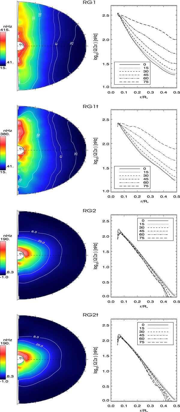
Figure 10. Left column: temporal and longitudinal average of the angular velocity profile achieved in cases RG1, RG1t, RG2 over 1 rotation period, and of RG2t over 1/2 rotation period. The reference frame rotation rate Ω/2π is 41.4 nHz (a tenth solar) for cases RG1 and RG1t, and 8.3 nHz for cases RG2 and RG2t. The isorotation line corresponding to the frame rotation rate is indicated on the plots, and corresponds to the second isorotation curve from the right for cases RG1 and RG1t and to the first isorotation curve from the right for cases RG2 and RG2t. Right column: radial profiles for selected latitudes (0, 15, 30, 45, 60, and 75 deg) for cases RG1, RG1t, RG2, and RG2t.
Download figure:
Standard image High-resolution imageIn Figure 11, we show latitudinal profiles of Ω for cases RG1 and RG2 at four different instants along with the average formed over the whole temporal interval sampled (solid line). The various curves correspond to temporal averages formed over either successive one rotation periods for RG1 or over temporal intervals of hundreds of days compatible with the period of time for which RG2 possesses one or multiple meridional cells (see below Section 4.2). We note the relatively good stability of the profiles found for RG1 over several convective overturning times and rotation periods (except near the polar regions due to the small level arm there making it difficult to form meaningful averages), thus confirming the well equilibrated state reached by this case. For case RG2 the situation is less obvious, with clear departure from the mean at given instant mostly because this case undergoes a large dynamical oscillation due to its slow rotation rate that we discuss in length in Section 4.2. Note however the much smaller range of variation as a function of latitude found in that case (30 nHz) with respect to case RG1 (200 nHz). This is due to the peculiar angular velocity profile realized in this model.

Figure 11. We display at mid-convection zone for cases RG1 (left) and RG2 (right), the angular velocity as a function of latitude for four different temporal intervals along with the average over the full temporal range sampled (solid line). For RG1 we display four consecutives 1 rotation period averages, and for RG2 we have chosen the temporal intervals corresponding to Figure 14 with either one or two meridional circulation cells. We clearly note that the angular velocity profile for RG1 is stable except near the polar regions, whereas the oscillating behavior of RG2 lead to significant departure of the angular velocity profiles at each instant with respect to the longest average.
Download figure:
Standard image High-resolution imageReturning indeed to Figure 10 (bottom rows) showing the angular velocity in the two cases rotating at a fiftieth of the solar rate, we note a large angular velocity contrast in radius solely due to the striking shellular state (i.e., angular velocity uniform on spherical surfaces) achieved by the simulations. Further, the rotation near the top edge of the computational domain is found to be retrograde in an absolute way, i.e., even taking into account the reference frame rotation. Given the large differences between cases RG1 (RG1t) and RG2 (RG2t), we have run verification models to be sure of the robustness of the results. For instance, we have progressively decelerated case RG1 to 1/50th the solar rate to check if we recover the shellular state achieved in case RG2. We find that when reaching a value of the convective Rossby number larger than about 1 (i.e., for a rotation around 1/15th solar), the influence of rotation on convection is reduced (as expected from earlier studies; Glatzmaier & Gilman 1982; Browning et al. 2004; Ballot et al. 2007; Brown et al. 2008). Thus, the cylindrical profile of the differential rotation observed in cases RG1 and RG1t is lost, the flow being less constrained to be quasi two-dimensional along the rotation axis. This has for direct consequence that such slowly rotating models do not show any angular velocity contrast in latitude.
Figure 12 presents the mean radial profile for the specific angular momentum obtained for each of our four models after averaging the angular velocity over longitudes and latitudes, and in time over one rotation period (except for case RG2t, averaged over all the iterations available). Also plotted on this view graph are the expected specific angular momentum profiles associated with uniform angular velocity profiles with Ω0 = 0.1Ω☉ (long-dashed triple dotted line) and Ω0 = 0.02Ω☉ (long-dashed line). The profiles achieved by models RG1 and RG1t are very similar both in shape and amplitude. Similarly, the profiles obtained for models RG2 and RG2t are also almost identical. This indicates that the distribution of specific angular momentum (and of the mean radial angular velocity) achieved in the simulations is not influenced by the turbulent state (e.g., Reynolds number) of the simulations up to the values that we have been able to compute. This is a quite different behavior compared to the solar convection, where lowering the diffusivities while keeping Pr constant in order to increase Re by a factor of 2 leads to some modification of the angular velocity profile (see Figure 4 of Brun & Toomre 2002). On the other hand, the specific angular momentum distribution achieved in our convective shell strongly depends on the bulk rotation considered. For models RG1 and RG1t with a bulk rotation a tenth of the solar value, the profile presents a positive slope throughout the computational domain. In these models, due to the cylindrical profile of Ω (see Figure 10), the radial contrast at high latitudes is smaller than at the equator so that these latitudes contribute to soften the mean radial profile presented in Figure 12.

Figure 12. Specific angular momentum profiles throughout the computational domain for the four simulations. These profiles are obtained by averaging the vϕ component of the velocity field over latitude, longitudes, and time. The averages are computed over the last rotation period for cases RG1 and RG1t, and over two-thirds of a rotation for case RG2t. Overplotted are the profiles that would be obtained if the angular velocity profiles were uniform over the convective shell with values of 1/10th and 1/50th of the solar value.
Download figure:
Standard image High-resolution imageThe specific angular momentum profile for the slower cases RG2 and RG2t is radically different, with a change of slope below r ≈ 0.2 R* and a negative slope in the outer part of the computational domain. This is directly related to the shellular rotation existing in these simulations. At small radii, the angular velocity is large, and although its radial mean profile has a negative slope, the contribution of the increasing radius (i.e., the specific angular momentum scales as Ωr2) maintains a positive slope for the specific angular momentum j. Moving toward the top of the domain, the mean radial angular velocity dramatically drops at all latitudes in these slowly rotating simulations (the total variation of Ω(r) at all latitudes is of more than 2 orders of magnitude; see Figure 10), decreasing faster than the increase of the radius, and leading to the observed change of slope. Near the top of the convective shell the absolute retrograde rotation seen in Figure 10 leads to a second change of slope in the mean radial profile of specific angular momentum.
Let us finally note that none of our simulations approach the extreme cases of uniform mean radial specific angular momentum or uniform mean radial angular velocity, as have been assumed in the modeling of angular momentum transport in the convective envelopes in one-dimensional stellar evolution models.
4.2. Structure of Meridional Flows
Another important large-scale flow established in rotating convective envelopes is the mean (axisymmetric) meridional circulation (i.e., the flow in the r–θ plane). This flow is maintained by small imbalance between latitudinal pressure gradient, Coriolis force acting on the differential rotation, Reynolds stresses, and buoyancy forces in the purely hydrodynamical case (e.g., Miesch 2005; Brun & Rempel 2008). In the Sun, this relatively weak flow (with respect to the solar differential rotation) is thought to play an important role in setting the solar cycle (Jouve & Brun 2007). It also plays important role for the redistribution of angular momentum, even though it only contains about 0.5% of the total kinetic energy (Brun & Toomre 2002). By contrast, in our RGB simulations we find that the kinetic energy contained in the meridional circulation (MCKE) accounts for about 8% of the total kinetic energy (see Table 2 and Figure 2) and thus cannot be neglected in the energy balance of our convective envelope. We display in Figure 13 the axisymmetric streamlines along with the radial and latitudinal components of the mean (axisymmetric) velocity for the four cases analyzed in the present paper. Again the rotation plays a significant role in shaping the flow properties, leading to a clear difference in the realized meridional circulation profiles. For cases RG1 and RG1t, we find a very stable profile consisting of one large single cell per hemisphere. Each cell is directed toward the pole at the top of the domain and toward the equator deeper down. Near the star's rotation axis the flow is mostly radial (vertical), and near the equator it is directed perpendicular to that axis. The contour maps reveal that the axisymmetric 〈vr〉 and 〈vθ〉 components (with 〈 〉 denoting longitudinal average) are of the same order of magnitude, with 〈vθ〉 being antisymmetric with respect to the equator and 〈vr〉 symmetric. For cases RG2 and RG2t, the picture is completely different. Due to the large dipole in the temperature maps (cf. Figure 4), the meridional circulation consists of one large single cell spanning the whole shell. The direction of this flow is different for models RG2 and RG2t, and depends on the latitudinal fluxes (see below). In both cases, there is no radial transport in the equatorial region. The amplitude of 〈vr〉 and 〈vθ〉 are larger than in the faster rotating cases (1000 m s−1 versus 700 m s−1). Due to its peculiar topology, the radial and latitudinal components of the mean velocity have opposite symmetries with respect to the equator and cases RG1 and RG1t.

Figure 13. First row: longitudinally averaged meridional circulation represented as streamlines, and contour plots of the radial 〈vr〉 and latitudinal 〈vθ〉 components of the meridional circulation velocity further averaged over time (one period) for cases RG1, RG1t and RG2, and over a third of a rotation for case RG2t. Solid and dashed contours denote counterclockwise and clockwise circulation, respectively. The color scale is the same for both contour plots in each row and is given by the color bars.
Download figure:
Standard image High-resolution imageTable 2. Representative Velocities, Energy Contents, and Differential Rotation Contrast
| Model |  |
 |
 |
 |
 |
 |
KE | DRKE | CKE | MCKE | ΔΩ |
|---|---|---|---|---|---|---|---|---|---|---|---|
| RG1 | 1348 | 1015 | 1406 | 848 | 2202 | 1780 | 1.3 × 10⁶ | 4.7 × 10⁵ (36%) | 7.1 × 10⁵ (55%) | 1.2 × 10⁵ (9%) | 78.9 |
| RG1t | 1370 | 1040 | 1456 | 914 | 2263 | 1803 | 1.3 × 10⁶ | 4.6 × 10⁵ (36%) | 7.2 × 10⁵ (56%) | 1.1 × 10⁵ (8%) | 64.7 |
| RG2 | 1905 | 1097 | 1511 | 1455 | 2670 | 2586 | 2.37 × 10⁶ | 1.5 × 10⁵ (6%) | 2.11 × 10⁶ (90%) | 1.0 × 10⁵ (4%) | 4.2 |
| RG2t | 1939 | 1188 | 1380 | 1343 | 2666 | 2552 | 2.15 × 10⁶ | 1.4 × 10⁵(6.5%) | 1.85 × 10⁶ (86%) | 1.6 × 10⁵ (7.5%) | 4.4 |
Notes. Temporal averages of the rms velocity  , of the rms components
  ,
,  ,
,  , and of fluctuating velocities
  and
and  (axisymmetric components are removed) are estimated at mid-layer depth, all expressed in units of m s−1. For cases RG2 and RG2t that undergo a long-term oscillation of KE, we have chosen to form the temporal average over a period representative of the simulations by avoiding peak (min/max) values. Also listed are the time average over the complete volume of the total kinetic energy KE and that associated with the (axisymmetric) differential rotation DRKE, the (axisymmetric) meridional circulation MCKE, and the nonaxisymmetric convection CKE, all in units of erg cm−3. The latitudinal contrasts between 0° and 60° of angular frequencies ΔΩ, quoted in nHz, are computed at the top of the domain.
Download table as: ASCIITypeset image
We also find that depending on the period over which the time average is performed, the pattern of the meridional circulation will present one or two cells in models RG2 and RG2t.
In order to illustrate the rich dynamics operating in the slowly rotating case RG2, we display in Figure 14 the temporal evolution of the meridional streamlines along with the temporal traces of the kinetic energy densities (KE, DRKE, CKE, and MCKE) over an interval of 2500 day near the end of the total evolution of the simulation. This allows us to identify the phases in which model RG2 possesses more than one large single cell. It turns out that the appearance of a second cell in the southern hemisphere is linked to a weakening of MCKE with respect to DRKE. When MCKE becomes smaller than DRKE we find a multicellular meridional circulation profile similar to that achieved in cases RG1 and RG1t, for which DRKE is always larger than MCKE. On the contrary when MCKE is larger than DRKE, situation that occurs often and lasts over a much longer periods of time as illustrated in the figure (over the ranges a and c), the meridional flow possesses one big clockwise cell. We believe that the reduced rotational constraint in the slowly rotating case RG2 is at the origin of such an intriguing behavior by allowing the meridional circulation to evolve freely. Further the oscillating meridional circulation patterns are likely a consequence of the convective structures that are clearly influenced by the strength and the location of the self-established temperature dipole (Figure 14).

Figure 14. Meridional circulation for case RG2 as a function of time over 2500 day late in the evolution of the simulation. The streamlines meridional cuts are obtained by averaging in time over the periods indicated by the associated letters on the energy plot on the left.
Download figure:
Standard image High-resolution image5. ANALYZING THE DYNAMICS
As we have seen in the previous sections our simulations possess a very rich dynamics. In this section, we aim to analyze and understand how such a complex and nonlinear behavior comes about. We will thus discuss the redistribution of energy, angular momentum, and heat in our convective shell in order to assess which physical processes are dominant in establishing the convective patterns and large-scale flows observed in our simulations.
5.1. Energetics of the Convection
Analyzing the kinetic energy budget contained in the turbulent convective motions is very useful to understand key features of our simulations, such as convection and large-scale flows, and how they vary with the model's parameters. As we have seen in Figure 3, the large stratification present in our models leads to an inward kinetic energy flux, with fast concentrated downflows overwhelming the slow broad upflows in transporting the kinetic energy. Indeed, the kinetic energy flux Fk scales as vrv2 so it is sensitive to the sign of the radial velocity component vr, and as vr in downflows is larger than in upflows, it yields when averaging over horizontal surfaces this asymmetric (downward) transport of the kinetic energy. The slowly rotating cases possess a more vigorous convection, with faster rms velocities (about a factor 1.3 higher) as indicated in Table 2 (and also Figure 8). Associated with these faster flows we also find that cases RG2 and RG2t possess a larger inward directed kinetic energy flux than their faster rotating counterparts (RG1 and RG1t). Converted to luminosity the kinetic energy flux reaches −120% (compared to −50%) of the total luminosity leading to an extremely large convective luminosity of 220% (compared to 140%; see Figure 3). Here, again the stabilizing effect of rotation on convection plays a central role in limiting the amplitude of the flows and thus the strength of Fk in cases RG1 and RG1t. Even if we compare case RG1 to case RG2 which have the same Reynolds number, the asymmetry between upflows and downflows is stronger in the slowly rotating case RG2.
To get a better insight on how the kinetic energy is redistributed among the various axisymmetric and nonaxisymmetric motions, we again split the KE into it components DRKE, MCKE, and CKE. We have already partly discussed the different behavior of these components in Section 4.2 via Figure 13. We report in Table 2 the volume and time-averaged values of KE and its components for the four cases discussed in the paper. These values reveal a strong difference between cases RG1 (RG1t) and RG2 (RG2t). The kinetic energy associated with the differential rotation DRKE represents a third of the total kinetic energy KE in cases RG1 and RG1t but only 6% in models RG2 and RG2t, where the kinetic energy density is essentially concentrated in the (nonaxisymmetric) convection itself. This is again due to the mild influence of rotation on convection in these simulations with slow bulk rotation. As the bulk rotation rate increases, more kinetic energy is diverted to longitudinal flows (i.e., differential rotation), and much less so in the meridional flows. It is striking to note that MCKE in slowly rotating case is close to DRKE and leads to fascinating modulation of the dynamics as seen in Section 4.2 and Figure 14. In cases RG2 and RG2t, the contribution of the mean flows to the total kinetic energy budget is noticeably weak and the convective motions are mostly nonaxisymmetric. Further these two cases exhibit an oscillation of their total kinetic energy that lasts about a rotation period. The difference between evaluating the rms velocities over a period of time for which KE is minimum or maximum is or order 3%–5%. Since case RG2t is slowly emerging from a pronounced deep of KE this explains why in Table 2, some of the rms velocities for this case are smaller than in RG2. Nevertheless given the smaller kinetic viscosity used in RG2t, overall this case has a larger Reynolds number (cf. Table 1) and is effectively more turbulent than RG2.
Another useful information on the turbulent properties of convection can be retrieved by plotting the kinetic energy spectra as a function of the spherical harmonic degree ℓ as was done in Figure 15. In this figure, we clearly see that the difference of amplitude between the large (low ℓ degree) and the small scales is important. It involves many orders of magnitude, thus confirming the well-resolved character of our simulations. For the fast rotating cases, the profiles present a plateau at low ℓ degree and the maximum of the energy distribution is located around ℓ = 10. None of these features exist for cases RG2 and RG2t. Quite interestingly these more slowly rotating cases display a conspicuous peak at ℓ = 1 that dominates all the other scales. This points toward the dipole in temperature and velocity seen in the Mollweide maps of Figure 4, in the three-dimensional rendering of Figure 5 and in the equatorial slices of Figure 7. As previously mentioned, this is expected since in his linear study of the onset of convection in spherical shells of various thickness, Chandrasekhar (1961) has demonstrated that the ℓ = 1 mode is among the easiest mode to excite when the topology is close to being a full sphere with an aspect ratio rmin/rmax equal or close to zero. It is important to realize that our simulations are fully nonlinear as demonstrated by the energy spectra, but that nevertheless the ℓ = 1 mode remains a dominant convection mode since our choice in our models of a small aspect ratio (i.e., rmin/rmax = 0.1) favors low ℓ modes.

Figure 15. Kinetic energy spectra for cases RG1t and RG2t averaged, respectively, over 1 and 1/10th of a rotation period.
Download figure:
Standard image High-resolution image5.2. Redistribution of Angular Momentum
Convection not only transports heat but also redistributes angular momentum. We seek here to understand the mechanisms responsible for the transport of angular momentum within our rotating convective shells yielding the differential rotation discussed in Section 4.1. With our choice of boundary conditions (see Section 2.1), no net torque is applied to the shell and the total angular momentum must be conserved. We indeed find that in our four simulations the total angular momentum averaged over the whole volume is conserved to within 10−7.
The transport of angular momentum may be assessed by considering the mean radial and latitudinal angular momentum fluxes  and
and  . Following Elliott et al. (2000) and Brun & Toomre (2002), the expression of these fluxes is extracted from the ϕ component of the momentum equation after averaging in time and longitude (denoted by the symbol
  ; see also Palacios & Brun 2007):
 (resp.
  ) is the flux associated with viscous transport,
  (resp.
  ) that related to Reynolds stresses, and
  (resp.
  ) represents the angular momentum flux due to meridional circulation. As was done in Brun & Toomre (2002), we then integrate respectively each flux over colatitude and radius to assess the net flux through a sphere of varying radius and through cones of varying inclination:
These integrated fluxes are presented in Figure 16 for our cases RG1 and RG2, and have been averaged over 8.5 rotation periods. For simplicity we drop the letter I when discussing the individual contribution of the flux.
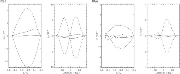
Figure 16. Time average of the latitudinal integral of the radial angular momentum flux  and of the radial integral of the latitudinal angular momentum flux
  for cases RG1 (left panels) and RG2 (right panels). The fluxes have been decomposed into their viscous (dash triple dotted), Reynolds stresses (dotted-dashed), and meridional circulation (dashed) components. The solid curves represent the total fluxes and serve to indicate the quality of the stationarity achieved. The positive values represent a radial flux directed outward, and a latitudinal flux directed from north to south. The fluxes have been averaged over 8.5 rotation periods in each case. The radial integrated fluxes for each cases have further been normalized by R2*.
Download figure:
Standard image High-resolution imageFor the faster case RG1, the radial flux  is strong due to the two cells pattern, yielding a strong radial transport in the equatorial regions. Despite some viscous transport associated with the radial shear, the angular momentum fluxes are mainly the result of a balance between the inward flux due to Reynolds stresses and the outward flux due to meridional circulation. The Reynolds stresses thus extract angular momentum from the surface and speed up the inner region whereas the meridional circulation flow, mostly directed outward at the equator, does the opposite job and extracts momentum from the deep inner parts.
Turning to the latitudinal fluxes, angular momentum is transported equatorward by Reynolds stresses, that act against the poleward transport by meridional circulation. This is consistent with the poleward streamlines existing in each hemisphere that corresponds to a counterclockwise circulation in the northern hemisphere. A small equatorward viscous transport occurs in both hemispheres due to the direction of latitudinal variation of Ω.
For case RG2, the radial transport of angular momentum by meridional circulation is weak. Indeed, for this slowly rotating simulation, the meridional circulation becomes unicellular, with one big cell covering the whole convective shell, and no radial transport is achieved in the equatorial regions, which are the regions that contribute the most in the integration of the radial fluxes. On the other hand, the viscous transport becomes important, related to the strong radial shear existing in this model in absence of radial transport by meridional circulation. The mechanisms yielding important transport of angular momentum are thus viscous terms balancing the Reynolds stresses, a configuration which is radically different from that achieved in model RG1 due to the very peculiar form of the meridional circulation appearing in the slowly rotating models. Let us note however that the net radial flux of angular momentum achieved in case RG2 is similar in amplitude to that achieved in case RG1. The transport due to Reynolds stresses is weaker in case RG2 compared to case RG1 because in that simulation, the convective pattern is less dominated by north–south aligned banana cells, and develops a more isotropic flow in which correlations are weaker.
The latitudinal fluxes are less symmetric with respect to the equator in case RG2, due to the large single cell of meridional circulation. The temporal average encompasses periods during which a second cell appears in the southern hemisphere (e.g., Figure 14), which translates into some weak latitudinal transport of angular momentum in this hemisphere. Similar to what is obtained for case RG1, the latitudinal flux balance is mostly between Reynolds stresses and meridional circulation because shellular rotation leads to almost zero viscous transport.
In both directions and for both cases, we note that the different processes balance each other so that the simulations tend to reach a statistical equilibrium in which almost no net flux is found in the radial or latitudinal direction. Due to the nonlinearity present in our turbulent simulations, it is to be expected that the total net flux of angular momentum (represented by the solid lines) is not strictly zero everywhere. However, averaging over several rotation periods leads already to a fairly good balance, confirming the mature state of the analyzed solutions.
5.3. Latitudinal Heat Flux Balance
We now turn to discussing the transport of heat with latitude achieved in our RGB models. We find that there are large fluctuations of temperature and entropy in our simulations. In Figure 17, we present temporal and longitudinal averages of the temperature fluctuations for cases RG1 and RG2. In model RG1, we find an organized symmetric pattern with respect to the equator, consisting of a warm equator and cooler poles. On the other hand, the northern hemisphere in RG2 is mostly hot while the southern hemisphere is cold, leading to an anti-symmetric temperature fluctuations profile consistent with the presence in this model of a dominant ℓ = 1 mode. Again there is a clear dichotomy between the two series of models, the cases rotating faster having smaller fluctuations and a more structured (banded) thermodynamic background.
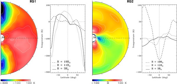
Figure 17. Temporal and longitudinal averages for cases RG1 and RG2 of the temperature fluctuations, accompanied by latitudinal profiles at three different depths in the computational domain. The results have been averaged over 1 rotation period in each case. The white contours for case RG1 indicate the levels with T ranging from −300 K to 100 K by step of 50 K. The white contours for case RG2 indicate the levels with T ranging from −50 K to 60 K by step of 10 K.
Download figure:
Standard image High-resolution imageConvective motions under the influence of rotation lead to efficient transport of heat in latitude or what is sometime referred to as anisotropic heat transport (Rüdiger et al. 2005). As with the transport in radial direction (see Figure 3), several physical processes contribute to the transport of heat in latitude. In order to determine which physical processes dominate in our models we have derived a new diagnosis in the ASH code allowing us to assess the latitudinal energy flux balance. By taking the scalar product between the velocity  and the Navier–Stokes equation (see Equation (2)) one can derive the equation for the temporal evolution of the kinetic energy (Heyvaerts 1998; Miesch 2005). By adding the heat equation (see Equation (3)) to the kinetic energy equation and after some algebra consisting in putting under a flux conservative form some of the terms (Heyvaerts 1998), one gets the anelastic equation for the total density energy (Miesch 2005):
where  is the internal density energy,
  is the kinetic density energy,
  is the work against the stratification, and F is the total energy flux. The
  term comes about because of anelastic formulation (see Bannon (1996) for a modified anelastic formulation in which the equation of state is altered to make that term disappear). F can be decomposed into several contributions:
the various terms being in turn heat transport by viscous stresses, by entropy eddy diffusion, by radiative diffusion, along with the kinetic energy and enthalpy fluxes. By assuming stationarity and that there is no net mass flux through horizontal surfaces, i.e.,  (with 〈 〉θϕ denoting an horizontal average), such that
  vanishes, one is left with the simple flux conservation equation
  .
.
In the latitudinal direction, Fθ has the following expression (Elliott et al. 2000; Rüdiger et al. 2005; Miesch 2005):
One may further decompose the kinetic and enthalpy fluxes into their mean and fluctuating components in order to isolate the contribution coming from the mean meridional circulation. Assuming that v can be decomposed into an axisymmetric (mean) part denoted 〈v〉 and a fluctuating contribution denoted v', it can easily be shown that:
where we recall that the temperature fluctuations T with respect to the background reference temperature  possesses a non-vanishing axisymmetric mean (e.g., 〈T〉 ≠ 0) as already discussed in Figure 17. For the kinetic energy flux, we similarly get:
We will assume that the last term of the two above expressions corresponds to the latitudinal transport of mean enthalpy and kinetic energy by the mean meridional (latitudinal) flow. We then integrate over the radius r for each θ (as we did in Section 5.2), to get the net flux through cones of various colatitudes and deduce the latitudinal heat flux balance. Figure 18 displays the balance obtained for cases RG1 and RG2. For the faster model RG1, we see that the turbulent Fe (we omit the θ index for simplicity) is transporting heat poleward while both the turbulent Fk and its mean part (cf. Equation (14)) are warming up the equator balancing the turbulent Fe. The mean enthalpy flux Fe,m=0 (cf. Equation (13)) is constant with poleward heat transport, helping its turbulent counterpart. All the other terms contribute little to this latitudinal transport. For case RG2, the overall picture is messier and significantly different. The mean enthalpy flux plays a more important role certainly because of the large one cell meridional circulation established in that model, while strikingly enough the fluctuating one is almost negligible (i.e., has almost no net latitudinal effect). The turbulent Fk is now poleward while its mean contribution remains equatorward thus in the same direction as the mean enthalpy flux. The balance achieved in this model is not as good as in RG1 mostly due to the fact that the model possesses larger temporal fluctuations and that several terms of comparable amplitude contribute to the latitudinal heat transport. Similar results for the more turbulent cases RG1t and RG2t are found. In summary, we note that in all models a subtle latitudinal heat balance between the various processes is established, involving mostly the enthalpy and kinetic fluxes and that their relative importance including their mean and turbulent contributions is clearly influenced by the rotation rate.

Figure 18. Energy flux balance as a function of latitude, obtained after performing a radial integral of the latitudinal fluxes further averaged in time for case RG1 (left panel) and RG2 (right panel). The averages are computed over 8.5 rotation periods in each case. The net flux is separated into five components: latitudinal enthalpy flux Fe and meridional enthalpy flux (m = 0 mode) Fe,m=0, latitudinal radiative flux Frad, latitudinal entropy diffusion flux Fed, latitudinal kinetic energy flux Fk, and latitudinal viscous flux Fnu (see Equations (12)–(14)). The fluxes are normalized with respect to the square of the star's radius.
Download figure:
Standard image High-resolution image5.4. Quality of Thermal Wind Balance Achieved
In rotating convection, both radial and latitudinal heat transport occur, as we have just discussed, establishing latitudinal gradients in temperature and entropy within the convective zone (see Figures 17 and 18). A direct consequence of these gradients is that the surfaces of pressure and density fluctuations will not coincide anymore, thereby yielding baroclinic effects. We can turn to the vorticity equations (Pedlosky 1987; Zahn 1992) to analyze the role of the turbulence and baroclinic effects in setting the large-scale flows discussed in Section 4. Briefly summarized, the baroclinic terms drive meridional flows that under the influence of Coriolis force yield longitudinal flows also known as the thermal wind. These baroclinic terms may also lead to a departure from cylindricity of the angular velocity profiles by braking Taylor–Proudman constraint (Pedlosky 1987).
The thermal wind balance equation can be derived from the vorticity equation as discussed in detail by Brun & Toomre (2002) and Miesch et al. (2006). The equation for the vorticity ω = ∇ × v in the purely hydrodynamical case can be derived under the anelastic approximation by taking the curl of the momentum equation (Equation (2); see also Fearn 1998 and Brun 2005 for its magnetohydrodynamic (MHD) generalization and the notion of magnetic (thermal) wind), it reads
with  the absolute vorticity,
  the vorticity in the rotating frame, and
  the viscous tensor (Equation (4)).
The ϕ component of the vorticity equation helps understanding the relative importance of the different processes acting in the meridional planes (Brun & Toomre 2002). In the stationary case ( ), and assuming an axisymmetric configuration (
 ) the azimuthal component of Equation (15) is
where  and
and
In the above expressions, we have omitted for the sake of clarity the 〈 〉 denoting the axisymmetric average.
Here, we have identified several contributions to characterize the shape of the angular velocity along the z-axis that we display (only for the dominant term) in Figure 19 for case RG1 and in Figure 20 for case RG2: Stretching describes the stretching/tilting of the vorticity due to velocity gradients; Advection describes the advection of vorticity by the flow; compressibility describes the stretching of vorticity due to the flow Compressibility;  is the baroclinic term;
  results from departure from adiabaticity; Viscous accounts for the diffusion of vorticity due to viscous stresses. Figure 19 displays for RG1 the left-hand side of Equation (16), along with the dominant terms of the right-hand side, their sum and the difference RHS − LHS. The first point to notice is that the thermal wind balance, which would be achieved in the stationary case by having a strict equality between the LHS and the baroclinic term, is not achieved in our simulation (contrary to what we find in most of the solar convective envelope Brun & Toomre (2002)). We note that LHS ∼ RHS which is a hint of the mature dynamical state of the model. The dominant terms for the evolution of vorticity also involve both turbulent transport by advection thus emphasizing the key role played by turbulent convection in setting the angular velocity profiles as discussed in Section 5.2. The viscous stresses contribute in key regions (mostly at the top of the domain) where the isocontours of Ω are distorted. Overall all these large terms cancel each other thus resulting on isocontours of Ω in RG1 that are close to cylinders as observed. A similar analysis of RG2 reveals again that there is no strict thermal wind balance. Large advection terms oppose the baroclinic contribution with compressibility also playing a role. The quality of the achieved balance is not as good in part due to the fact that the meridional flows possess large fluctuations that make temporal average less meaningful, with the direct consequence that the temporal derivative of ωϕ cannot be neglected as easily. The shellular shape of the differential rotation in the slowly rotating cases RG2 and RG2t is clearly neither cylindrical nor conical, and it is unclear given their large convective Rossby number (cf. Table 1) and the weak influence of rotation on their dynamics whether their angular velocity profile can be usefully analyzed with the thermal wind balance contrary to RG1 and RG1t, for which the diagnosis is more adequate. We thus conclude that even though the amplitude of the baroclinic effect is large, it does not play a role in shaping the angular velocity profile as important as in solar simulations, at least at the rotation rates that we have explored in this study.
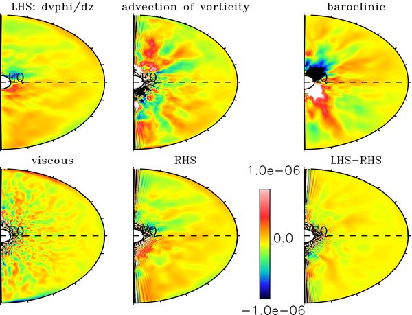
Figure 19. Temporal and longitudinal average for case RG1 of the derivative of along the z-axis  and of the main components of the right-hand side of this very same equation, namely, the compressibility term, the baroclinic term and the viscous term, and of the complete right-hand side of Equation (16). The last shell on the bottom right shows the difference of the left-hand side and theright-hand side The color bar applies to all panels.
Download figure:
Standard image High-resolution image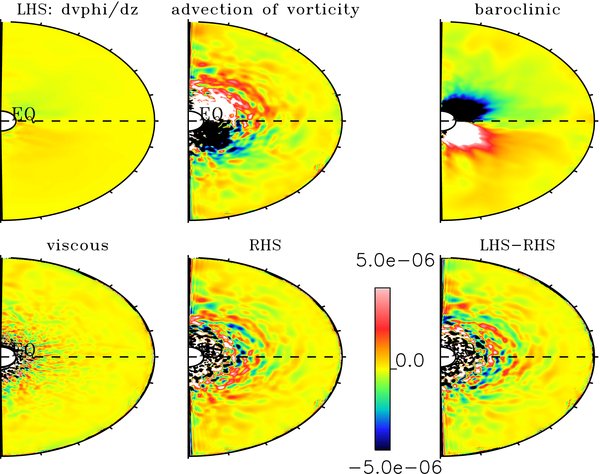
Figure 20. Same as Figure 19 for case RG2. Temporal average has been performed over 800 days.
Download figure:
Standard image High-resolution image
6. SUMMARY AND PERSPECTIVES
We have presented the first three-dimensional anelastic simulations of the deep stratified convective envelope of a RGB star aimed at understanding the interplay between rotation and turbulent convection. Despite the relative simplicity of our models, they can give us a first hint on the intricate dynamics of these extended convective envelopes and of the subtle interplay between convection and rotation. We have in particular been able to test the sensitivity of our simulations to change in the bulk rotation rate and/or to the Reynolds number.
Convection displays a rich dynamics in red giant stars, and this appears clearly both in our rotating simulations and in earlier works that did not include rotation (Porter & Woodward 2000; WPJ03). The achieved convective patterns are characterized by broad upflows surrounded by a complex network of downflow lanes. The total number of cells obtained at mid-depth of the convective envelope of a giant is about ten at most, in overall agreement with the star-in-a-box simulations of the CoBOLD group. Although an overall coherence of the convective structures exist in the entire convective shell, the large aspect ratio existing between the top and bottom of these huge envelopes implies a change of the convective pattern with depth with a fast disappearance of the interconnected downflow network present at the top of the simulated domain. Associated with these convective cells are large temperature and velocity fluctuations. They lead to a huge enthalpy, e.g., convective, flux reaching up to 200% and more of the total flux emerging at the top edge of the shell, thus compensating for the large downward flux of kinetic energy due to the high degree of stratification assumed in our simulations. The importance of this downward flux of kinetic energy has also been observed in other simulations of turbulent convection (Chan & Sofia 1989; Cattaneo et al. 1991; Woodward et al. 2003), and indicates a clear contradiction with one of the main assumptions of the MLT used in one-dimensional stellar evolution codes, according to which the kinetic energy flux can be neglected and the convective luminosity is set to be the total luminosity (i.e., Lconv = Ltot = L*) in convection zones.
Testing two different bulk rotation rates, we have also been able to point the strong sensitivity of the heat and angular momentum distribution to this parameter. In the slowly rotating cases, more relevant to the rotation rate of the reported RGB star observations, a large ℓ = 1 temperature dipole is established that leads to the separation of the convective shell in two zones of respectively divergence and convergence of the horizontal flow. Such a dipolar configuration also shows through the radial velocity of the fluid, and is very similar to the dipolar behavior observed in nonrotating simulations of turbulent convection (Kuhlen et al. 2006; WPJ03; FSD02). When accelerating to a bulk rotation of a tenth solar, the dipole no more dominates the energy spectra by itself but instead a large plateau of dominant ℓ's develops.
The bulk rotation rate also affects the resulting large-scale flows, namely, differential rotation and meridional circulation. Meridional circulation is found to possess two large cells (one per hemisphere) or one large cell encompassing the overall domain when rotation is slow. This structure is associated with the temperature dipole existing in these slowly rotating cases, for which the rotational influence is not large enough yet to shape (constrain) the turbulent convection (i.e., the convective Rossby numbers is greater than 1; see Table 1). Differential rotation possesses large radial gradients in both faster and slower cases, and the achieved profile does not vary when changing the Reynolds number by a factor of about 3. On the other hand, the latitudinal rotation profile is very sensitive to the rotation rate such that the cylindrical profile existing for moderate rotation is reshaped into a shellular rotation profile with no latitudinal gradient for the slowly rotating cases.
The differential rotation profile can be analyzed considering the quality of the achieved thermal wind balance in the simulations. The cylindricity of the rotation achieved in the moderately rotating cases is a consequence of the advection terms of the vorticity equation canceling out the baroclinic effect. On the other hand, in slowly rotating cases where the rotation profile is shellular, there is no clear influence of the baroclinicity, and the thermal wind diagnosis does not appear to be appropriate. In neither cases is a strict thermal wind balance achieved.
Finally, we have for the first time produced an analysis of the latitudinal energy balance in our simulations. Together with the angular momentum transport, one can say that Reynolds stresses play a key role in redistributing heat, energy, and angular momentum. In the slowly rotating case, meridional circulation flows are large and influence greatly the dynamical balance with the mean axisymmetric transport contributing more than the fluctuating enthalpy or kinetic energy fluxes.
This works opens a large field of perspectives both in the domain of (magneto-)hydrodynamical simulations of turbulent convection in the very peculiar conditions of deep extended stellar envelopes, and in the domain of stellar evolution.
Both the finding of overluminous convective flux (due to a large negative kinetic energy flux) and of nonuniform mean radial angular velocity profiles in our simulations is of prime importance for one-dimensional stellar evolution models with rotation. As discussed in the introduction, these models normally assume that the convective regions, with convection described by the MLT formalism (with Lconv = L*), rotate uniformly, i.e., Ωconv(r) = cst. However, changing this assumption will influence the efficiency of (shear-induced) turbulent transport in the underlying radiative interior of giants as they undergo dredge-up episodes, and may thus have an impact on their surface chemical composition (see Palacios et al. 2006 for details). In a forthcoming paper, we will thus analyze the impact of such a result on one-dimensional rotating stellar evolution models.
Of course the three-dimensional models discussed in this work are still relatively simple descriptions of RGB stars and we must be cautious when extending their results to the conditions found in real stars, but we intend to progressively improve their realism. These can be achieved by doing for instance the following improvement: one possibility could be to add a stable radiative shell at the bottom of our computational domain in order to better understand its coupling and how angular momentum is redistributed between the two zones. Also extending the thickness of the spherical shell so as to reach radii closer to the actual surface of a giant star would help to ground the results presented here. Finally, we are aware that the presence of magnetic fields (which have actually been detected at the surface of giant stars) is likely to alter the overall picture (at least the achieved rotation profiles) that we have described in this purely hydrodynamical study. We thus intend in a the near future to consider MHD simulations of the envelope of red giant stars and to study dynamo action and the generation of turbulent and large-scale magnetic fields.
We thank C. Charbonnel for kindly providing the one-dimensional stellar evolution model, and thank her together with J.-P. Zahn & M. S. Miesch for useful discussions and comments about this paper. The simulations were carried out using the french supercomputing facilities of CCRT at CEA and Idris at CNRS via the GENCI agency. This work received financial support from the Programme National de Physique Stellaire of CNRS/INSU (France), and was also supported by a post-doctoral fellowship from CEA Saclay (France) awarded to A.P. This work is part of the STARS2 project (http://www.stars2.eu) founded by a grant of the European Research Council awarded to A.S.B. We acknowledge the use of the SDvision software (Pomarede et al. 2008) to generate the three-dimensional rendering shown on Figure 5.
Footnotes
- 4
Even though stars lose mass as they ascend the RGB, the rate of mass loss remains very small up to the He flash, and should thus not lead to a large variation of the angular momentum that we will assume conserved.