


ABSTRACT
The mysteries of near-Earth asteroid 4179 Toutatis have been more comprehensively unveiled by analyzing the optical images taken during the Chang'e-2 flyby in 2012. Compared with previous works, this paper concentrates on the photogrammetric relation between the Chang'e-2 spacecraft and Toutatis and the imaging shadow effect during the flyby. Accurate models of imaging and optical measurements are developed to study Toutatis's dimensions and rotational state at the time of imaging. As the illumination study shows, the shadowed region perpendicular to the long axis accounts for 27.78% of the Toutatis images, while the long axis of the body is fully captured. With a compensation on the shadow effect, the optical measurements reveal that Toutatis's long axis is 4354 ± 56 m, the maximum length is 4391 ± 56 m, and the spatial orientation described with the angles of direction cosine during the flyby is (126 13 ± 029, 12298 ± 021, 12663 ± 046). Furthermore, a new triaxial ellipsoid of 4354 × 1835 × 2216 m and a volume of 7.5158 km3 are proposed based on the previous Toutatis shape model. The effectiveness of the proposed method is validated, since typical features such as the neck and endpoints agree well with the results simultaneously observed by the ground radar. Moreover, it also potentially provides a feasible approach to precisely calculate the spin period of Toutatis.
Export citation and abstract BibTeX RIS
1. INTRODUCTION
An accurate measurement of an asteroid's dimensions is of great significance in order to study the formation and evolution of small celestial bodies (Morbidelli et al. 2002). Meanwhile, with a deeper understanding of the threats posed by near Earth asteroids (NEAs), scientific communities, and even the United Nations, have shown increasing concern over the observation, detection, and scientific study of NEAs.6 An NEA is considered a potentially hazardous object7 (PHO) if its minimum orbit intersection distance (MOID) with respect to the Earth is less than 0.05 AU (approximately 19.5 lunar distances) and its diameter is larger than 100 m. Hence, an exact estimation of the geometric parameters of an NEA is important to evaluate the degree of its potential impact (Betzler & Borges 2012). Toutatis, an Apollo-, Alinda-, and Mars-crossing NEA with an Earth MOID of 0.006 AU8, is listed as a typical PHO, large in size and close to the Earth. Since it was discovered in 1989, many observational approaches, such as early infrared radiometric observation (Spencer et al. 1993; Davies et al. 2007), optical observation through ground photometry (Spencer et al. 1995; Lupishko et al. 1995) and the Hubble Space Telescope (Noll et al. 1995), and the current mainstream ground-based delay-Doppler radar observations (Ostro et al. 1995, 1999; Hudson et al. 2003; Takahashi et al. 2013), have been tried successfully as it passed by the orbit of the Earth every four years.
Toutatis's exact dimensions, such as its dynamical characteristic of Non-Principal Axis Spin (NPA; Hudson & Ostro 1995; Mueller et al. 2002), are always the concern of astronomers. Spencer et al. (1993) estimated effective dimensions of 2 km by 2.5 km from two-dimensional (2D) images via infrared radiometric measurements. Noll et al. (1995) measured a 2D dimension range of 1.7–2.4 km using Hubble. The UBVRI polarimetry observation by Lupishko et al. (1995) estimated about 3 km in radius. However, the accuracy and the resolution of these early passive optical measurements were limited by the observational quality. Using a dynamically equivalent, equal-volume ellipsoid (DEEVE) model and based on several high-resolution radar images, Hudson and Ostro (Ostro et al. 1995; Ostro et al. 1999; Hudson et al. 2003) fitted a complete radar-observation-based shape model (hereafter referred to as the shape model) with dimensions of 4.60 × 1.92 × 2.29 km and an uncertainty of ∼100 m. The shape model is refined based on 1992–2008 radar-based images (Takahashi et al. 2013), and the dimensions are updated as 4.46 × 1.88 × 2.27 km with an uncertainty of ∼100 m (Huang et al. 2013a). The shape model based on the radar measurements has been widely accepted, although the results might also be affected by the observing distance and incomplete coverage of the body surface.
All of the above observations were conducted on or near the Earth, with a distancelarger than 0.01 AU. On 2012 December 13, China's Chang'e-2 spacecraft took a close flyby of Toutatis for the first time and took a set of high-resolution photos (Huang et al. 2013b). The Chang'e-2 spacecraft, launched on 2010 October 1, was originally designed as a lunar orbiter. After orbiting around the Moon for 20 months, it had completed the scheduled tasks, such as stereo imaging for the whole lunar surface and landing point detection. After that, the spacecraft was still in good condition, so it left the Moon and began a series of missions. First, it flew to the Sun–Earth L2 point, and then it flew by the asteroid Toutatis. The nearest distance during the flyby was only 1.6 km (Tang et al. 2013). The optical images of the peanut-shaped asteroid captured by Chang'e-2 during its flyby provide a valuable opportunity to understand the basic geometric and physical information of Toutatis at close range with optical measurements. Meanwhile, the American National Radio Astronomy Observatory (NRAO) observed clear ground-based delay-Doppler radar images (Takahashi et al. 2013). These fortuitously orchestrated simultaneous observations of Toutatis with multiple observational techniques provide precious data that can be used to verify past analyses and even be blended with each other to help unveil the mysteries of Toutatis.
After Chang'e-2's optical detection, Zou et al. (2014) estimated the orientation through a series of the canny operator based matching between the optical images and simulated images from the shape model, which is about (− 338, 330, 471) ± 1o in the expression of 3-1-2 Euler angles in the shape model coordinate system. Further, Huang et al. (2013a), based on the approximate orientation from the shape model and taking into account the imaging strategy during the flyby, statistically estimated the dimensions of Toutatis to be 4.75 × 1.95 km with an uncertainty of 10%, namely, ∼475 m. These estimation results verified the previous conclusions within a comparatively wider margin of error, yet were insufficient to create a brand new picture about the dimensions of Toutatis. Huang et al. (2013a) pointed out that the narrow field angle of the camera onboard Chang'e-2 and the high local resolution of the optical images created difficulties in the three-dimensional (3D) surface modeling.
Accounting for particular constraints of Chang'e-2's shooting pictures during the flyby, the size of Toutatis can be better estimated. This paper analyzes the effectiveness of the optical images with radar observation data as auxiliary, and proves the completeness of the imaging along the long axis. Afterward, making use of key constraint relations between a series of images, Toutatis's dimensions are obtained with an uncertainty of 56 m and its orientation with an uncertainty of 055 about the long axis from 6.9 million kilometers away from the Earth. Using these accurate dimensions and orientation as reference, and combining with the radar-based shape model, the volume and spin period of Toutatis can be further estimated. The relevant methods and results contribute to the comprehensive understanding of Toutatis's characteristics, as well as precisely evaluate the threats thereof.
The rest of the paper is organized as follows. In Section 2, we sketch out the flyby geometry of Chang'e-2 relative to Toutatis according to tracking, control, and imaging during flyby. In Section 3, we analyze Toutatis's imaging completeness and identify its long axis from optical images combined with the refined shape model from radar observations. In Section 4, we provide an imaging constraint based measurement model and analyze the uncertainties. Then, we show measurement results in Section 5 and provide some deeper discussions in Section 6. Finally, in Section 7, we present the conclusions.
2. OBSERVATION AND FLYBY RELATIONSHIP
2.1. Observation and Imaging
After departing from the Sun–Earth L2 point, Chang'e-2 had been flying for approximately eight months before flying by Toutatis. The flyby happened at 8:30 (UTC) on 2012 December 13, about one day after Toutatis's periodical flyby of the Earth at 6:40 (UTC) on 2012 December 12. The minimum flyby range from the Earth is 0.046 AU, about 18 times the average distance from the Earth to the Moon. At the moment of flyby, Chang'e-2 was more than 6.9 million kilometers away from the Earth.
To ensure a successful flyby, the Beijing Aerospace Control Center (BACC) had corrected the trajectory of Chang'e-2 several times before the detection, the last of which greatly shortened the theoretical flyby range from hundreds of kilometers to several kilometers, and obtained a relative velocity of 10.73 km s−1. During the flyby, the ground observation systems and control systems were used to track and measure the movement of Chang'e-2 and Toutatis. The spacecraft orbit is tracked through the radiometric data, and the asteroid's orbit is determined through the ground optical telescopes.
A CMOS camera with a focal length of 54 mm, a resolution of 1024-by-1024 pixels, and a field of view (FOV) of 72 by 72 was used in the experiment. After Chang'e-2 departed the Sun–Earth L2 point, imaging tests and parameter calibration were conducted using fixed stars. Chang'e-2 started to take photos of Toutatis after passing by it with a mode of vanishing point gaze (Huang et al. 2013b); the effective imaging time was approximately 100 s, and the imaging frequency was 5 frames per second. Several hours before the flyby, the attitude of Chang'e-2 was adjusted to make sure Toutatis came into the view of the camera and that communication with the Earth was well established. In addition, the constraint on the solar panels–Sun angles was met. The orientation of the Chang'e-2 spacecraft remained fixed inertially throughout the imaging campaign.
2.2. Flyby Relation
When imaging an asteroid with a space-borne camera, the orientation of Toutatis is a function of the relative state/dynamics, which are the position/velocity and the rotation between Chang'e-2 and Toutatis. Strict motion relations of relative displacement and relative rotation based on orbit data provide possibilities to high-precision optical measurement and analysis.
2.2.1. Relative Displacement
After the last orbit trimming, Chang'e-2 became a man-made Earth-crossing asteroid in the solar system with an orbital period of about 16 yr. The orbital period of Toutatis is around four years. During the imaging time of 100 s, the perturbation sources most influencing the relative velocity between Chang'e-2 and Toutatis were the gravity of the Sun, the solar radiation pressure, the gravity of Jupiter, and the gravity of Toutatis. The former three will perturb the relative velocity of 3.96 × 10⁻⁴ m s−1, ∼10−5 m s−1, and 3.78 × 10⁻⁷ m s−1, respectively. A change in relative velocity during the flyby can be calculated based on the gravitational parameter of Toutatis. Supposing the gravitational parameter of Toutatis is 1.279 × 10⁻⁶ km3 s−2 (Scheeres et al. 1998) and the flyby range is larger than one kilometer (Tang et al. 2013), the change in relative velocity is less than 2.56 × 10⁻⁵ m s−1. In conclusion, the relative velocity change caused by different gravity sources is less than 4.7 × 10⁻⁴m s−1. That is to say, in 100 s, there was a relative rectilinear motion of 1073 km, whereas the lateral displacement caused by various perturbation forces was only 4.7 cm. Therefore, during the flyby, Chang'e-2 and Toutatis moved in a way very similar to uniform linear motion, with an uncertainty of 4.4 × 10⁻⁶%.
2.2.2. Relative Rotation
During the imaging, Chang'e-2 kept a constant attitude. The telemetry attitude data returned by Chang'e-2 show that the changes in roll, pitch, and yaw attitude were all below 10−4 radians during the imaging time. Furthermore, irregular spin is one of the typical characteristics of Toutatis. It has two spin periods around its long axis and principal axis of 5.41 and 7.33 days, respectively (Hudson & Ostro 1995). During the effective imaging time of 100 s, high-resolution imaging lasted for only 20 s. Toutatis spun around the two axes for 00114 and 00154, respectively. In the optical images, the dimension of Toutatis is less than 400 pixels, which means that the difference caused by the spin of Toutatis in the optical images is less than 0.054 pixel. Therefore, during the high-resolution imaging time, Toutatis kept a fixed attitude with an uncertainty of 1.4 × 10⁻³% s−1. In conclusion, during the Chang'e-2 flyby of Toutatis, it can be considered that there was no relative rotation between the two.
3. IMAGE ANALYSIS
Our interest here lies in understanding the total coverage of the illuminated surface and whether the general shape is captured in the images or if it is even possible to identify it in our data.
3.1. Related Coordinate Systems
Three types of coordinate systems are involved herein, namely, an inertial coordinate system, a camera coordinate systems, and a spacecraft body coordinate system. For the convenience of the following analysis, they are uniformly described here. In an inertial space, various tracking data, including the coordinates and velocities of the Sun, the Earth, Toutatis, and Chang'e-2, are unified into the heliocentric inertial system Oi − xyz. The relative motion relation between Toutatis and Chang'e-2 as well as the relative rotational dynamics are described in the original camera coordinate system  . The optical center of the space-borne camera at the moment of initial imaging is the origin
  , and the optical axis of the camera at the moment is the z-axis. Real-time camera coordinate systems
  are built for each imaging position, the origins of which are located at the camera realtime optical centers, respectively. Here, the original camera coordinate system is distinguished from the real-time camera coordinate systems for the former, which is regarded as a fixed frame in the following vision-based calculation. The conversion between the original and real-time camera coordinate systems can be achieved via constraint-based visual calculation. The conversion between the heliocentric inertial system and the camera coordinate systems relies on the body coordinate system Ob − xyz, that between the inertial coordinate system and body coordinate system is based on the attitude transfer matrix, and that between the spacecraft body coordinate system and camera coordinate systems is achieved based on the camera installation matrix. The spatial relationships among the three types of coordinate systems are shown in Figure 1.
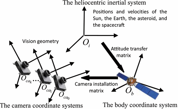
Figure 1. Coordinate systems and their relationship.
Download figure:
Standard image High-resolution image3.2. Illuminated Area on the Surface
Assuming that there is no light transmission on Toutatis's surface, when the imaging distance is long, lines of sight and solar rays can, respectively, be considered to be parallel vectors. When Toutatis is treated as a rotating body around the long axis, the visual range of the surface of the equivalent rotating body can be described by the dihedral angle θ formed by the interface of Sun rays and that of lines of sight. The spatial geometric relation of θ is shown in Figure 2, where n1 are the normal vectors of the boundary plane of Sun rays, n2 the normal vectors of the boundary plane of lines of sight, and  ,
,  , and
, and  are the vectors of Sun rays, lines of sight, and Toutatis's long axis in the original camera coordinate system, respectively. The computation of θ is described in Appendix A.1.
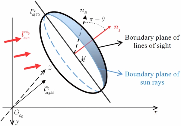
Figure 2. Spatial geometric relation of the vectors based on the equivalent rotating body.
Download figure:
Standard image High-resolution imageWhen the orientation of the long axis is limited in a rough degree range, the dihedral angle θ of the visible surface of the rotating body was calculated to be from 122° to 180°. From the spatial geometric relationship, the conclusion can be thereby made that the long axis of Toutatis can fortunately be completely reflected on the Chang'e-2 optical images, whereas the edge of the upper right part perpendicular to the long axis is partly shadowed.
3.3. Identification of the Long Axis
Based on data from several radar observations since 1992, Takahashi et al. (2013) studied Toutatis's inertia moment and verified the high-resolution shape model (Hudson et al. 2003) using the observation in 2012. The shape model provides a good reference for marking Toutatis's long axis in optical images captured by Chang'e-2. First, based on the solar line-of-sight angle, the illuminated surface of the shape model was simulated. Then, the attitudes of the shape model's three axes were rotated to achieve the most correspondence with the observed optical images of Toutatis. Then, the first order estimate of the direction of the axis of Toutatis was identified in the optical images. It is emphasized here that the long axis cannot be extremely precisely identified due to uncertainties in the shape model and the resolution of the optical images. In this paper, the two landmarks A and B along the long axis are considered the endpoints of the long axis. Figure 3 shows the attitude and landmarks, respectively, in the shape model and Chang'e-2 image.
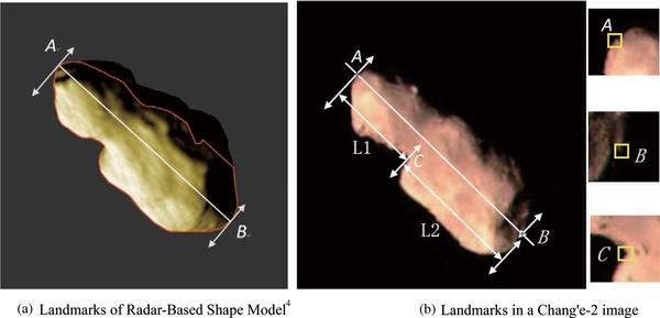
Figure 3. Comparison between images from Chang'e-2 and the radar-based shape model. (a) Landmarks of the radar-based shape model. (The radar model is from http://echo.jpl.nasa.gov/asteroids/shapes/hirestoutatis.obj.) (b) Landmarks in a Chang'e-2 image.
Download figure:
Standard image High-resolution image4. MEASUREMENT MODEL
Since the images only differ from each other in depth, the almost parallax-free imaging relation shows that the three-dimensional calculation barely yields any matching errors. However, since the resolutions of the images obviously dropped as Chang'e-2 flew away from Toutatis, it is difficult to achieve accurate matching between corresponding image points. Under such paradoxical circumstances, bundle adjustment, the commonly used photogrammetric method, is limited in eliminating errors to realize high-precision measurement. Therefore, in this paper, based on the relative motion and relative geometry of Toutatis and the spacecraft, several strict imaging constraints are introduced to the multi-view calculation to remove the effects of major uncertainties by matching and calculation.
4.1. Multi-view Calculation Based on Imaging Constraints
The relative motion between Chang'e-2 and Toutatis leads to a special imaging relationship. That is, all lines between homonymy points at different spatial coordinates intersect at an infinite point P∞ that indicates the translational direction in space. Furthermore, on the image planes, the lines through homonymy landmarks at different positions intersect at one point, epipole e, which is the projection of P∞. Based on the relation between the image sequence and the spatial motion, the constraints and the computational algorithm can be developed.
During the imaging period, the principal point coordinate and the focal length of the space-borne camera are deemed as known and stable with even exposure at each time of imaging. According to the observing geometry, three strict constraints can be proposed for accurate modeling.
The scale constraint. During any two times of continuous imaging, the relative motion of the spacecraft and Toutatis is unchanged. Therefore, Δam, n, the relative displacement vector of the camera between the picture  and the picture
  , can be expressed as

where δt is the time interval between two camera exposures that could be accurately controlled by the high-precision clock equipment on the spacecraft, and v is the relative velocity vector between Chang'e-2 and Toutatis. When tracking Chang'e-2 using ground communication, errors, including systematic error and random error, are inevitable. Nevertheless, the measurement accuracy of the relative velocity in a short time could reach the mm s−1 level, which provides the baseline accuracy for the whole measurement system.
The attitude constraint. According to the relative rotation relation between Chang'e-2 and Toutatis, if a unit matrix I[3 × 3] of the first image Img0 is established as the reference, the camera rotation matrix Rk of any other image Imgk could also be uniformly expressed as

The epipole constraint. Theoretical values of em, n, the epipole coordinate, between any two optical images Imgm and Imgn in the sequence are identical and can be uniformly denoted by

Incorporating the scale constraint, the attitude constraint, and the epipole constraint into the solution of multiple view geometry, the coordinate of a spatial point P in the original camera coordinate systemcan be obtained. Appendix A.2 gives a detailed description of the solution. The camera matrices Pm and Pn can be obtained by combining with a pure translational imaging model. The specific process refers to the multi-view geometry principle (Hartley & Zisserman 2004). After getting the camera matrix of each optical frame and coordinates of homonymy image points of the spatial point P, the exact spatial position of P in the original camera coordinate system can be obtained.
4.2. Precise Estimation of Key Feature Points
According to the above geometric relationship, the computation accuracy is directly determined by the accuracy of the coordinates of key feature points, including the homonymy landmarks and the epipole. Although the measurement accuracy of each individual point is low, the specific imaging model and constraint relations during Chang'e-2's flyby of Toutatis could help to improve the estimation accuracy of the feature points. The epipole can be estimated using the two-point algorithm with the least squares criterion (Li et al. 2000). Accurate registration of homonymy landmarks can be realized, according to a motion constraint based filter algorithm. The following first theoretically gives a motion constraint within the sequence of homonymy image landmarks. Then, based on the theoretical relation, the pixel coordinates of the homonymy landmarks are estimated accurately using a polynomial-based filter.
The motion constraint for the filter. The 2D image coordinate [uP(t), vP(t)]T of any spatial point P on Toutatis's surface and its spatial 3D coordinate ![${\bf X}_P^{c_0 } \left(t \right) = \left[ {x_P \left(t \right),y_P \left(t \right),z_P \left(t \right)} \right]^T$](https://content.cld.iop.org/journals/1538-3881/149/1/21/revision1/aj502685ieqn9.gif) in the original camera coordinate system meet the following continuous time-varying relationship, the detailed derivation of which is given in Appendix A.3.
in the original camera coordinate system meet the following continuous time-varying relationship, the detailed derivation of which is given in Appendix A.3.


where uP(t) and vP(t) are the pixel coordinates of the row and column direction at time t, fu and fv are the camera equivalent focal lengths in the two directions, u0 and v0 are coordinates of the camera principle point, and V = ||v|| represents the relative speed.
The relationship between the homonymy landmarks [ui, vi]T, i = 1, 2, ..., n of each image can be accurately established through Equations (4)–(6), which lay the theoretical foundation for the accuracy of the homonymy landmarks. However, since  is unknown, the exact coordinates of the landmarks cannot be calculated via Equations (4)–(6) directly. Fortunately, there was a favorable condition that
  was constant in the original camera coordinate system. Therefore, to analyze the time-varying rule of the image coordinates of homonymy landmarks, different constant values can be assigned to
  . Using the scale constraint, the image points xk = [uP[k], vP[k]]T, k = 1, 2, ..., n change continuously and stably with time sample k, which can be approximated with a polynomial.
The filter for the homonymy landmarks was designed according to the rule of approximate polynomials. First,  was set as a constant, and the theoretical formula in Equations (4)–(6) was used to precisely calculate pixel coordinates of the image point sequence xk; then, a high-order polynomial was used to fit xk, and the values of the polynomial functions were used as an estimate of xk. Figure 4 shows a comparison of mean square errors of image coordinates of different sequence lengths via polynomials of different orders. Each statistical point was based on 200 random sample points of
  . The figure shows that for sequences of the same length, the error converges as the order of the polynomial is increased; for sequences of the same fitting order, the error diverges with an increase in the sequence scale. When the order of the polynomial is above 7, in the sequence scale of 60 points, the mean square error is less than 0.004 pixel. Therefore, fitting polynomials with orders of more than seven can be used as filter functions for an accurate correction of the homonymy landmarks.

Figure 4. Effectiveness of different filter functions.
Download figure:
Standard image High-resolution image4.3. Uncertainties
The aggregate uncertainties of the optical imaging during flyby need to be addressed. The source errors include uncertainties in the relative dynamics of Toutatis and spacecraft and the measurement models. The uncertainties in the relative dynamics are determined by that of the motion relation in Section 2. Their effects on the measurement system have proved to be negligible. Therefore, the measurement uncertainty is primarily determined by the uncertainty of the measurement model.
According to the measurement model, the main errors include the matching error of homonymy landmarks, the estimation error of the epipole, and transmission errors. To precisely analyze the degree of error, a ground testing platform is developed based on the relative imaging relationship and actual parameters including relative velocity, exposure time, and camera parameters.
The ground testing platform, on one hand, could generate theoretical spatial coordinates of simulated landmarks and corresponding homonymy image points at each exposure time. On the other hand, after adding noise to the simulated data, it can realize a series of processes including filtering and spatial position calculating, as well as a comprehensive analysis of transfer relations of various error sources.
The spatial coordinates of Toutatis's endpoints are basic landmarks for calculating the dimension and the orientation of the long axis. Based on the exact measurement model and Monte Carlo method, the uncertainty of the endpoints can be obtained statistically via the ground testing platform after estimation of the epipole, filtration of the homonymy image points, and error transmission.
The cumulative variance of a parameter can be computed as shown in the following equation. The uncertainty of the dimension dAB and the orientation αAB can be obtained from the coordinates of endpoints and their uncertainties

where τAB represents the function of Euclidean distance dAB or the orientation angle αAB between endpoint A and B, pi denotes the coordinates of A and B in the original camera coordinate system, and σpi denotes the variance of each coordinate.
Based on the above mathematical formulation, the optical measurement of Toutatis's long axis is achieved as follows. First, the endpoints of the long axis are identified. Then, the extracted endpoints are matched on the sequence images. In order to obtain enough precision under a limited image resolution, a filter is invoked. Then, the spatial coordinates of the endpoints are computed under the constraints. Finally, the dimensions and the orientation of the long axis on the optical images are calculated.
5. RESULTS
The results are organized as follows. Section 5.1 gives the results of the feature points, including endpoints and the epipole. Section 5.2 gives the calculation of Toutatis's dimension and orientation along the long axis. Section 5.3 contains an accurate computation of the illumination and shadow.
5.1. Estimation of the Feature Points
A total of 30 continuous images with relatively high resolution were used for final processing. The initial matching of homonymy image points is achieved on the biquadratic interpolation images by virtue of corner-based matching algorithms, ensuring a maximum error not greater than 1 pixel and a standard deviation not greater than 0.35 pixel. After filtering of homonymy points' coordinates based on the motion constraint, the mean error declines from 0.39 pixel to 0.06 pixel, and the standard deviation declines from 0.4 pixel to 0.05 pixel. The spatial position error of the endpoints caused by matching errors could be calculated statistically on the basis of the measurement transfer relation. After filtering, the order of magnitude of the calculated standard deviation of the spatial position decreases from hundreds of meters to ∼10 m. When errors are described by the rms, errors on the x, y directions in the original camera coordinate system are ∼2 m and that on the z direction is ∼60 m; thus, the error is mainly reflected in the z direction, namely, the depth direction. Table 1 shows estimated coordinates of endpoints A and B before and after filtering.
Table 1. Estimation Results of Endpoints A and B
| ID | xA1 | yA1 | zA1 | xB1 | yB1 | zB1 | LA1B1 | xA2 | yA2 | zA2 | xB2 | yB2 | zB2 | LA2B2 |
|---|---|---|---|---|---|---|---|---|---|---|---|---|---|---|
| (m) | (m) | (m) | (m) | (m) | (m) | (m) | (m) | (m) | (m) | (m) | (m) | (m) | (m) | |
| Img1 | −1866 | −383 | 64619 | 734 | 1983 | 66145 | 4136 | −1846 | −381 | 63966 | 733 | 1995 | 66543 | 4353 |
| Img2 | −1822 | −383 | 66409 | 762 | 1988 | 68320 | 3995 | −1820 | −379 | 66105 | 759 | 1999 | 68688 | 4357 |
| Img3 | −1796 | −377 | 68508 | 788 | 1992 | 70394 | 3981 | −1794 | −374 | 68255 | 785 | 2004 | 70832 | 4354 |
| Img4 | −1767 | −372 | 70305 | 808 | 1992 | 72309 | 4030 | −1768 | −368 | 70401 | 810 | 2008 | 72977 | 4353 |
| Img5 | −1743 | −369 | 72759 | 839 | 2003 | 74897 | 4108 | −1742 | −364 | 72546 | 837 | 2012 | 75122 | 4353 |
| Img6 | −1716 | −365 | 74685 | 858 | 1999 | 76486 | 3932 | −1716 | −360 | 74692 | 863 | 2016 | 77267 | 4353 |
| Img7 | −1687 | −359 | 76540 | 889 | 2003 | 78616 | 4066 | −1690 | −356 | 76836 | 889 | 2021 | 79415 | 4355 |
| Img8 | −1659 | −352 | 78343 | 914 | 2008 | 80796 | 4268 | −1665 | −352 | 78982 | 915 | 2025 | 81558 | 4352 |
| Img9 | −1635 | −354 | 80833 | 950 | 2023 | 83595 | 4468 | −1639 | −347 | 81127 | 941 | 2029 | 83702 | 4353 |
| Img10 | 1608 | −346 | 82767 | 973 | 2025 | 85599 | 4506 | −1613 | −343 | 83273 | 967 | 2034 | 85849 | 4352 |
| Img11 | −1581 | −341 | 84815 | 978 | 2003 | 86138 | 3715 | −1587 | −338 | 85418 | 992 | 2038 | 87996 | 4354 |
| Img12 | −1554 | −336 | 86827 | 1012 | 2019 | 88993 | 4102 | −1561 | −334 | 87561 | 1018 | 2042 | 90138 | 4353 |
| Img13 | −1525 | −330 | 88576 | 1044 | 2028 | 91463 | 4528 | −1535 | −330 | 89707 | 1044 | 2047 | 92292 | 4358 |
| Img14 | −1508 | −327 | 91773 | 1054 | 2014 | 92484 | 3544 | −1509 | −326 | 91847 | 1070 | 2051 | 94422 | 4352 |
| Img15 | −1481 | −326 | 93851 | 1065 | 2003 | 93745 | 3453 | −1483 | −322 | 93999 | 1097 | 2055 | 96572 | 4351 |
| Img16 | −1445 | −320 | 94817 | 1104 | 2027 | 97068 | 4133 | −1457 | −317 | 96142 | 1123 | 2060 | 98727 | 4358 |
| Img17 | −1426 | −317 | 97764 | 1141 | 2034 | 99315 | 3811 | −1431 | −313 | 98291 | 1149 | 2064 | 100861 | 4349 |
| Img18 | −1399 | −314 | 99775 | 1157 | 2021 | 100399 | 3518 | −1405 | −309 | 100436 | 1175 | 2068 | 103018 | 4357 |
| Img19 | −1372 | −309 | 101854 | 1235 | 2097 | 106960 | 6217 | −1379 | −304 | 102589 | 1200 | 2073 | 105168 | 4355 |
| Img20 | −1332 | −299 | 102227 | 1227 | 2058 | 106465 | 5483 | −1353 | −300 | 104719 | 1226 | 2077 | 107280 | 4344 |
| Img21 | −1305 | −296 | 104289 | 1262 | 2079 | 109661 | 6410 | −1327 | −296 | 106875 | 1252 | 2080 | 109424 | 4336 |
| Img22 | −1290 | −294 | 107746 | 1257 | 2040 | 109157 | 3732 | −1301 | −291 | 109019 | 1278 | 2085 | 111607 | 4360 |
| Img23 | −1257 | −285 | 108961 | 1329 | 2105 | 115022 | 7010 | −1275 | −287 | 111158 | 1303 | 2089 | 113711 | 4339 |
| Img24 | −1247 | −290 | 13204 | 1303 | 2032 | 112362 | 3551 | −1249 | −283 | 113308 | 1330 | 2094 | 115898 | 4361 |
| Img25 | −1198 | −271 | 112449 | 1439 | 2188 | 123891 | 11996 | −1223 | −278 | 115419 | 1356 | 2098 | 118057 | 4390 |
| Img26 | −1134 | −260 | 109966 | 1401 | 2107 | 120794 | 11370 | −1198 | −274 | 117612 | 1382 | 2103 | 120197 | 4358 |
| Img27 | −1122 | −265 | 113871 | 1410 | 2087 | 121439 | 8320 | −1172 | −270 | 119754 | 1407 | 2106 | 122307 | 4339 |
| Img28 | −1031 | −240 | 108267 | 1491 | 2167 | 128235 | 20270 | −1145 | −265 | 121858 | 1433 | 2111 | 124452 | 4363 |
| Img29 | −1086 | −260 | 120141 | 1512 | 2167 | 130177 | 10647 | −1119 | −261 | 123954 | 1458 | 2113 | 126498 | 4332 |
| Img30 | −799 | −189 | 91001 | 1444 | 2038 | 124043 | 33192 | −1095 | −257 | 126289 | 1484 | 2118 | 128647 | 4226 |
Notes. xA1, yA1, zA1, xB1, yB1, and zB1 are coordinates of the two endpoints in the original camera coordinate system before the motion constraint based filtering; xA2, yA2, zA2, xB2, yB2, and zB2 are coordinates of the two endpoints after filtering; and LA1B1and LA2B2 are the long axis dimensions of the two types of endpoints, respectively.
Download table as: ASCIITypeset image
The epipole is obtained from several pairs of random images. In order to ensure the reliability of the result, the image pairs with a small imaging distance and fewer homonymy points are filtered out and matching operators with scale invariant characteristics are adopted. Table 2 is the epipole estimation result in three color channels of the RGB format based optical images. Based on the transfer relation, the epipole estimation error of one times the STD leads to less than 30 m of calculation errors for the endpoints.
Table 2. Estimation Result of the Epipole
| Epipole | Channel R | Channel G | Channel B | Mean Value | STD | Transfer Error |
|---|---|---|---|---|---|---|
| (pixel) | (pixel) | (pixel) | (pixel) | (pixel) | (m) | |
| eu | 609.38 | 609.58 | 609.42 | 609.46 | 0.10 | <28 |
| ev | 528.16 | 527.99 | 528.21 | 528.12 | 0.11 | <30 |
Download table as: ASCIITypeset image
5.2. Dimensions and Orientation
Figure 5 shows the measurement results of identified endpoints A and B of six sequential frames arbitrarily selected from the above 30 continuous images under UTC time coordinates. Table 3 shows the measurement results of typical dimension features and the orientation of the long axis. Typical dimensions include the maximum dimension and the length of the two lobes by taking the long axis as the reference distance. The orientation of the long axis is described through the angles of direction cosine between the long axis and three coordinate axes of the original camera coordinate system. Based on the analysis in the analytical conclusion of Section 3, due to the shadowing of the images in the direction perpendicular to the long axis, the relevant dimension in this direction could be measured on the optical images but does not represent the real scale of Toutatis.

Figure 5. Measurement results based on identified endpoints of the long axis.
Download figure:
Standard image High-resolution imageTable 3. Dimensions and Orientation Based on Optical Images
| Parameters | Dimension (m) | Orientation of l4179(deg) | ||||||||||
|---|---|---|---|---|---|---|---|---|---|---|---|---|
| AB | Lmax | L1 | L2 | STDL | αl − x | STDl − x | αl − y | STDl − y | αl − z | STDl − z | STDα | |
| Projection Plane | 3491.7 | 3521.4 | 1427.6 | 2093.8 | 2 | 137.29 | 0.04 | 132.71 | 0.04 | / | / | 0.05 |
| Imaging Space | 4353.8 | 4391.4 | 1780.3 | 2611.0 | 56 | 126.13 | 0.29 | 122.98 | 0.21 | 126.63 | 0.46 | 0.55 |
Download table as: ASCIITypeset image
The dimension of the long axis measured using the optical method is 4354 m with an uncertainty of 56 m, a difference of 246 m compared to 4.6 ± 0.1 km (Hudson et al. 2003) and 106 m compared to 4.46 ± 0.1 km (Takahashi et al. 2013; Huang et al. 2013a). The longest dimension of Toutatis reflected by the image is 4391 m, and the error bar of 56 m is shorter than 100 m. The reasons for the difference include: (1) there exist deviations between identified long axis endpoints and the actual positions, whether they are based on the shape model or extracted from the optical image; (2) there may be a little shadow shelter at the bottom right of the optical images, and point B is slightly offset from the actual end point; and (3) there do exist certain deviations as to the measurement results of these two methods. The dimension of 4391 ± 56 m agrees with the length range of 4.75 km ± 10% estimated by Huang et al. (2013a), while the error bar has been greatly improved. The optical measurements presented here fully integrate much useful information and constraints of Chang'e-2 flying by at a close distance. Therefore, the measurement accuracy of Toutatis's dimensions is improved by comparing it with ground-based remote observations. Dimensions of Toutatis's three axes can be estimated through a proportional relation between the results of the optical measurement and that of the refined shape model, which is 4354 × 1835 × 2216 ± ∼ 56 m. This gives us more accurate estimate of the size of the asteroid.
The orientation of Toutatis's long axis in the original camera coordinate system has been estimated through the canny-based matching between Chang'e-2 optical images and images from the shape model by Zou et al. (2014), which is (− 338, 330, 471) ± 1° in 3-1-2 Euler angles, and (12791, 12300, 12481) ± 1° in the expression of direction cosine angles in the original camera coordinate system. Comparing it with the orientation of (12613 ± 029, 12298 ± 021, 12663 ± 046) calculated through optical approaches in Table 3, the deviations of the three direction cosine angles are (− 178, − 002, 182), respectively. This, on one hand, shows that Toutatis's attitudes measured through the two methods are basically consistent. On the other hand, through further comparison, some obvious differences could still be found between the optical images and the radar-based images, such as the tail of the larger lobe. Thus, some errors are introduced if considering the shape model based image as the reference for the canny operator based matching, especially in the depth direction. Therefore, the discrepancies in orientation between the two methods are insignificant overall, but the deviation of αl − z is larger comparatively. The spatial orientation contains rotation information, which is discussed in Section 6.2.
5.3. Illumination and Shadow
Based on the accurate coordinates of endpoints A and B, the shadow in the optical images could be precisely calculated. The dihedral angle of the visible part between the boundary plane of Sun rays and that of lines of sight calculated through the long axial vector and Sun ray vector is 12998, as shown in Figure 6(a). That is to say, if we consider a cylinder of equivalent size, about 27.78% of the body is hidden due to shadowing. Figure 6(b) is a prediction of the shadow in the optical images combined with a simulation image based on the shape model. Comparing Figure 6 and the previous Figure 3(a), the calculated shadow is consistent with the simulation result based on the shape model.
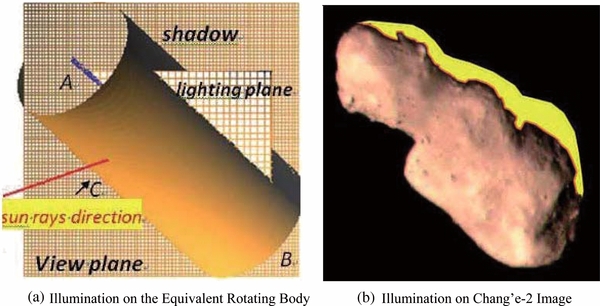
Figure 6. Results of calculated visible part on Toutatis's imaging surface. (a) Illumination on the equivalent rotating body. (b) Illumination on the Chang'e-2 image.
Download figure:
Standard image High-resolution image6. DISCUSSIONS
6.1. Volume, Mass, and Density
Toutatis's dimension can be obtained through the optical method, but due to incomplete coverage of Chang'e-2 images, the volume of the asteroid cannot be estimated directly. Fortunately, Ostro and Hudson's radar based shape model provides more accurate relative information on the shape. According to the cube law, we can scale Toutatis's volume based on the shape model by adjusting axes of Toutatis from 4.46 × 1.88 × 2.27 km to 4354 × 1835 × 2216 m. The new estimated volume is 7.5158 km3, 0.1830 km3 less than 7.6988 km3 by the refined radar based shape model. In addition, the newest radar observation and Chang'e-2 images show that Ostro and Hudson's shape model corresponds to Toutatis's actual shape over ∼97% of its volume (Takahashi et al. 2013), so if a more accurate shape model can be established based on the radar observation of 2012, the estimation of the volume will be more accurate.
Furthermore, based on the estimated volume, the mass of Toutatis can be recalculated. According to analysis results from the radar echo, Toutatis's density is between 2100 kg m−3 and 2500 kg m−3 (Scheeres et al. 1998; Ostro et al. 1999; Birlan 2002), so the mass is between 1.578 × 10¹³ kg and 1.879 × 10¹³ kg. Naturally, if the exact mass of the asteroid can be estimated according to other approaches, such as the Yarkovsky effect (Chesley et al. 2003), an accurate density can be calculated based on the volume, and the bulk composition and internal makeup of Toutatis can be further analyzed.
6.2. Spin Period
The equivalent rotating body at the time of the Chang'e-2 flyby can be simulated in the earth plane of sky as shown in Figure 7(a). Comparing this with the ground radar observations on 2012 December 12 as shown in Figure 7(b)9, it can be seen that endpoint A at the head of the smaller lobe, point C at the neck, and the sheltered endpoint B on the optical image correspond well to those on the radar image, indicating that the two images are identical in spatial orientation. Nevertheless, there exists a certain deviation as to the long axis orientations in the two figures. One reason for this deviation is the extracting error of the long axis endpoints. Another is that the imaging time of the optical image was about half a day later than that of the radar observation; therefore, after the radar observation in Figure 7(b), Toutatis had spun further, as described by Hudson & Ostro (1995).

Figure 7. Feature comparisons from different angles of view. (a) Converted equivalent rotating body. (b) NASA radar image.
Download figure:
Standard image High-resolution imageFurthermore, such disparity provides an opportunity for an accurate analysis of the spin period of Toutatis. The spin period can be calculated by taking the average rotation rate over the observation period. The change in attitude can be obtained by directly comparing landmarks such as A, B, and C in optical and radar images. If the images from the radar observation around 2012 December 13 can be obtained, then corresponding feature points of Toutatis can be found. Such an analysis would help improve the existing rotational dynamical models of Toutatis.
7. CONCLUSIONS
On 2012 December 13, Chang'e-2 successfully captured optical images of Touatis via a close flyby. This closest imaging has attracted many scientific communities' attention in unveiling mysteries of this PHO. In this paper, the dynamical model and optical measurements are rigorously developed. Our analysis investigated whether its dimensions and orientation could be accurately measured through optical images. Next, the shadow effect is investigated in order to validate that the optical image of Toutatis's long axis is fully captured. The internal relations between relative motion and imaging are introduced into the optical measurement model to ensure measurement accuracy. The measured dimension of Toutatis's long axis is 4354 m with an uncertainty of 56 m, the longest dimension is 4391 m with an uncertainty of 56 m, and the orientation of the long axis at the flyby time is (12613 ± 029, 12298 ± 021, 12663 ± 046) based on the direction cosine angles. From the point of view of measurement precision, the estimated dimensions and orientations are more accurate and acceptable than the previously published results. The disparity in the overall dimension is about 106 m, which is jointly caused by the shape model errors and the shadow effect. The three-axis dimensions, volume and mass, of Toutatis are re-estimated with nearly simultaneous earth radar observations and the dimension from the optical method. Furthermore, a quantitative study on the spin period may be feasible by fusing surface features from both the optical and radar images simultaneously.
In summary, the Chang'e-2 flyby near Toutatis has inspired a more accurate estimation of the geometrical mysteries of Toutatis, such as the dimensions and spatial orientation. All of these would further promote more comprehensive understanding of this remote and mysterious small body.
The authors are grateful to Dr. Michael W. Busch at NRAO for discussions, and Prof. Junze Liu and Hongbing Xu at the Spacecraft Operation and Management department of BACC for providing data. The authors acknowledge valuable comments and discussions with Yong Liu, Hang Wang, Shaoran Liu, Junqi Liu, Ye Liu, Jinchao Xia, Xie Li, Lue Chen, Songtao Han, Jin Sun, Hongzheng Cui, Baofeng Wang, Lei Liu, Mei Wang, Jia Wang et al. of BACC. We would especially like to thank the anonymous reviewer and the editors of The Astronomical Journal. The relevant work of this paper is jointly supported by the National Natural Science Foundation of China, 41204026, and China Postdoctoral Science Foundation.
APPENDIX: APPENDIX MATERIAL
A.1. Calculating the Visible Surface of the Rotating Body
In the original camera coordinate system, let the line-of-sight vector from the spacecraft to the body be  , the vector of Sun rays be
  , and the vector of Toutatis's long axis be
  ; then, the visible surface of the rotating body can be calculated using the following three steps.
A.1.1. Calculating the Boundary Plane of the Sun Rays
First, in the original camera coordinate system,  is determined by
  , the Sun centroid coordinate, and
  , the equivalent rotating body center, as

Then, define plane S1 as the plane that passes the main axis  and is co-planed with the vector of Sun rays
  and calculate the normal vector
  of the plane S1 with the following equation:

Then, define plane  as the plane that passes the main axis
  and is perpendicular to the plane S1, and calculate the normal vector
  of the plane
  using the equation

Finally, calculate the plane  , which passes the center point
  , and with
  as its normal vector, using the equation

Figure 8 is the sketch map of the boundary plane of Sun rays.
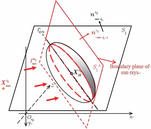
Figure 8. Sketchmap of the boundary plane of Sun rays.
Download figure:
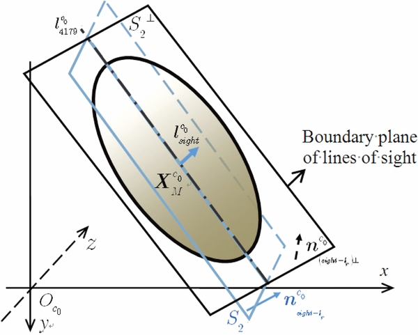
Standard image High-resolution imageA.1.2. Calculating the Boundary Plane of the Line of Sight
Figure 9 is the sketch map of the boundary plane of the line of sight. The boundary plane of lines of sight is calculated in the original camera coordinate system. Strictly speaking, any position on the Toutatis surface can correspond to a vector of the line of sight, yet its analysis and calculation are extremely complex. Because the distance from the spacecraft to Toutatis at the imaging time is much larger than the dimension of Toutatis itself, the vector of lines of sight  can be represented by the parallel beams passing through the origin and the center
  as
as

Figure 9. Sketch map of boundary plane of the line of sight.
Download figure:
Standard image High-resolution image
Define S2 as the plane that passes the cylinder main axis  and co-planes with the line of sight (directory vector
  ), and calculate the normal vector
  of the plane S2 according to the equation

Then, calculate the normal vector  of
of  , which is defined as the plane passes the cylinder main axis
  and is perpendicular to S2:

Finally, according to the below equation, calculate the plane  , which passes the point
  , and with
  as its normal vector:

A.1.3. Dihedral Angle between the Two Boundary Planes
The visible surface of the rotating body is directly determined by the dihedral angle θ between the boundary plane of the Sun rays and that of the line of sight. The angle θ can be calculated through the angle between the two normal vectors  and
and  with the following relationship:
For convenience, let n1 represent  , and n2 represent
  . Thus, we yield the following equations:


The part within θ could have been illuminated by the Sun and shot by the camera at the same time, which makes it visible in the optical images. Other parts are regarded as shadowed or regions that are not detected by the spacecraft camera.
A.2. Solution of Multiple View Geometry
Supposing P is a point on Toutatis's surface,  is the spatial coordinate of P in the original camera coordinate system, mP[3 × 1] is the homogeneous image coordinate of P in Imgm, and nP[3 × 1] the homogeneous image coordinate of P in Imgn. There exists the following relationship between the image coordinates and
  :
:


where Pm is the camera matrices of Imgm, Pn is the camera matrices of Imgn, is the pseudo-inverse of Pm, and
  is the pseudo-inverse of Pn.
If the camera position of Imgm is taken as the origin and the relative world coordinate system is built based on the reference of the optical axis direction at this moment, the camera matrices of Pm and Pn are expressed as follows, respectively:
whereRn is the camera rotation matrix of Imgn, an is the translation vector at Imgn's imaging position, and K is the inner orientation matrix of the camera, which is expressed as
A.3. The Relationship of the Image Coordinates and the Corresponding Spatial Coordinates
Use the homogeneous vectors [uP(t), vP(t), 1]T to formulate the image coordinates mP(t) of the motion point P that is in line with the relation model of movement and imaging herein. Use the homogeneous vectors [xP(t), yP(t), zP(t), 1]T to formulate the coordinate  in the original camera coordinate system. Based on the multiple-view geometrical relationship, there is a mapping relation between mP(t) and
  as follows:
According to the attitude constraint, whenever t > 0, the above relation can be simplified as follows:


where Vx(t),Vy(t),Vz(t), respectively, refer to the velocity components of the motion point P in the original camera coordinate system in the direction of x, y, and z.
According to the scale constraint,  in Equation (A.3.3) can be expressed as

where Tnorm is the normalized velocity vector of the motion point P in the original camera coordinate system, namely, the normalized coordinate of the Chang'e-2 spacecraft in the original camera coordinate system.
Introduce the essential matrix E according to the multiple view geometry, and establish the following relationship between Tnorm and E.

Based on the essential matrix's definition, combined with the epipole constraint, the formulation of E can be expressed as

where K and K' are camera inner orientation matrixes. As the same camera was used during this flyby, the formulation of K and K' becomes

Substitute Equation (A.3.8) into Equation (A.3.7); E can be derived thereby as
Then, the vector [TX, TY, TZ]T is yielded, and each component is as follows:
Subsequently, according to Equations (A.3.4) and (A.3.5),  is derived:
where 
Substituting Equation (A.3.11) into Equation (A.3.2), the conclusion can be derived:
Footnotes
- 6
- 7
Task Force on potentially hazardous Near Earth Objects, report of the Task Force on potentially hazardous Near Earth Objects (2000 September).
- 8
JPL Small-Body Database Browser: 4179 Toutatis (1989AC). Retrieved 2012–03–23.
- 9