


ABSTRACT
We investigate the fundamental parameters of age, distance, and mass function slope for the poorly studied clusters Koposov 1 and Koposov 2. These clusters were discovered recently and tentatively classified as globular clusters. Using the Large Monolithic Imager on Lowell Observatory's Discovery Channel Telescope, we present photometry extending to V = 25, three to four magnitudes below the main sequence turnoffs for the clusters. We find the clusters have tidal radii of 15 pc and 10.7 pc and distances of 34.9 kpc and 33.3 kpc for Koposov 1 and Koposov 2, respectively. Studying the stellar content of the clusters, we use completeness-corrected star counts to reveal extremely faint total magnitudes of 2.01 and 0.03 in V, and steep Salpeter-like present-day mass functions. Finally, we show that the spatial positions of the clusters agree well with the position of the Sagittarius stream and conclude that these two objects are open clusters removed from the Sagittarius galaxy.
Export citation and abstract BibTeX RIS
1. INTRODUCTION
Koposov 1 (Ko 1) and Koposov 2 (Ko 2) are two extremely small clusters originally discovered though a Sloan Digital Sky Survey (SDSS) search (York et al. 2000). Koposov et al. (2007) searched the SDSS Data Release 5 using a difference of two Gaussians method tuned to find small stellar overdensities. Initially classified as globular clusters, Ko 1 and Ko 2 were added to the rapidly growing list of small satellites in the Milky Way (MW) halo. In general, these MW satellites seem to fall into two categories. Some are small companion galaxies to the MW, such as SDSS J1049+5103 (Willman et al. 2005), the Bootes dwarf spheroidal galaxy (Belokurov et al. 2006), the Canes Venatici dwarf (Zucker et al. 2006a), the Ursa Major II dwarf (Zucker et al. 2006b), the Pisces II dwarf galaxy (Belokurov et al. 2010), and the four galaxies detailed in Belokurov et al. (2007). Other objects appear to be Galactic globular clusters (GGCs), such as Segue 1 (Belokurov et al. 2007) and Segue 3 (Belokurov et al. 2010; Fadley et al. 2011).
Globular clusters are some of the oldest known objects in the universe. Originally viewed as simple stellar populations with straightforward evolution schemes, they have been immensely useful laboratories for examining stellar evolution. Recent findings, however, have shown that analysis of these clusters is much more complicated than previously believed. Several systems classically described as globular clusters, such as ω Cen (Villanova et al. 2007) and M54 (Siegel et al. 2007), may, in fact, be remnant nuclei of dwarf galaxies disrupted through gravitational interactions with the MW. Gratton et al. (2012) provides extensive details on clusters with multiple populations, such as NGC 6397 (Milone et al. 2012) and many others, severely questioning whether any GGCs are actually simple populations. In addition to the problem of complex populations, analysis of globular clusters is complicated by their stellar dynamics. Over time, mass segregation concentrates higher-mass stars in the cluster core while the clusters lose stars due to evaporation and tidal stripping. This flattens the stellar mass function (MF), as seen in Paust et al. (2010). The assumption that old globular clusters would appear as a very sparse grouping of stars, as is seen in the Palomar 13 and AM 4 (Hamren et al. 2013), led to the conclusion by Koposov et al. (2007) that Ko 1 and Ko 2 were, in fact, heavily stripped globular clusters.
In this work, we examine the exact nature of Ko 1 and Ko 2 based on new deep photometry. On the basis of their size, present day stellar MFs, and location, we find it probable that the clusters are not heavily stripped globular clusters but, rather, they may be open clusters removed from the Sagittarius dwarf by tidal stripping of that galaxy. We outline the observations and image reduction in Section 2 and the photometry and calibration in Section 3. The color–magnitude diagram (CMDs) and luminosity functions (LFs) of the clusters and the meaning of the results are discussed in Section 4. We summarize our conclusions in Section 5.
2. OBSERVATIONS
Observations were collected using the Large Monolithic Imager (LMI) on the 4.3 m Discovery Channel Telescope (DCT) at Lowell Observatory. The LMI is a full-wafer 6 K × 6 K deep depletion e2V CCD specifically built for wide-field precise photometry. To match the seeing, the camera was binned 2 × 2, giving an effective pixel scale of 0.24 arcsec pixel−1 and a 12.5 arcmin × 12.5 arcmin field of view. Observations were taken over the span of two nights on 2013 April 2 and 3. Due to ongoing commissioning of the DCT at the time of the observations, the active mirror support and auto guiding systems were offline. To ensure focused, untrailed images, exposure times were limited to 10 minutes. We made nine 10 minute observations in both the V and I bands for both Ko 1 and Ko 2, with the exception of the I band for Ko 1, for which we have eight 10 minute observations. Despite the operational limits of the telescope, the average measured image point-spread function was 1.2 arcsec and several images were better than 1.0 arcsec. Images of the two clusters can be seen in Figure 1.
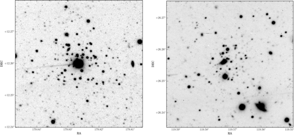
Figure 1. Ko 1 and Ko 2 are shown on the left and right, respectively. These images are four arcminute square cutouts from center of the LMI fields centered on the clusters. Both clusters are compact with small stellar populations. The star in the center of Ko 1 is a V = 14.2 mag foreground star. It has an HST guide star number of N6E8000018. A background galaxy partially obscures the center of Ko 2.
Download figure:
Standard image High-resolution imageTable 1 lists the images taken for this work. All of the observations were made under photometric conditions. Ko 1 and Ko 2 were observed at very low air masses, never rising above 1.10. The two standard fields, LC 53 and LC 71, were taken from the Smith (2001) compendium of Landolt (1992) standard stars. The LC 53 field was observed at an airmass of 1.77 and the LC 71 field was observed at 1.22 airmasses.
Table 1. Observations
| Date | Target | Exposures |
|---|---|---|
| 2013 Apr 2 | Ko 1 | 4 × 600 s in V |
| 4 × 600 s in I | ||
| Ko 2 | 6 × 600 s in V | |
| 6 × 600 s in I | ||
| 2013 Apr 3 | Ko 1 | 5 × 600 s in V |
| 1 × 60 s in V | ||
| 4 × 600 s in I | ||
| 1 × 60 s in I | ||
| Ko 2 | 3 × 600 s in V | |
| 1 × 60 s in V | ||
| 3 × 600 s in I | ||
| 1 × 60 s in I | ||
| LC 53 | 3 × 1 s in V | |
| 3 × 1s in I | ||
| LC 71 | 3 × 10 s in V | |
| 3 × 10 s in I |
Download table as: ASCIITypeset image
3. PHOTOMETRY AND CALIBRATION
All of the images were reduced using standard IRAF (Tody 1993) techniques using biases and twilight sky flats. The reduced images for each cluster were combined into master V and I images. The nine V images and eight I images of Ko 1 were summed to create master images. For Ko 2, we instead chose to average the nine V and I images. The difference in method changes the photometric zero point of the calibrations, but makes no difference in our analysis of the data. Photometry was completed on the master images using DAOPHOT/ALLSTAR (Stetson 1987). A final star catalog for each cluster was made by matching the V and I photometry and requiring that each star in the catalog had a photometric uncertainty of less than 0.1 mag in each filter. The resulting star catalogs had 2873 stars for the field around Ko 1 with a limiting magnitude of V = 26, and 1567 stars for the field around Ko 2 with a limiting magnitude of V = 25.
To calibrate the data, an aperture correction was applied to the DAOPHOT photometry using a 10 pixel aperture, chosen from curve-of-growth analysis. Using nine standard stars from the LC 53 field with (V − I) colors ranging from 0.017 to 2.084 and eight stars from the LC 71 field with colors from 0.623 to 1.143, we computed first-order color terms, airmass terms, and zero points for the cluster photometry. Using V and I as the calibrated magnitudes and v and i as instrumental magnitudes from a 1 s exposure, the photometric transformations were found to be


Examining the residuals of these equations with the standard stars, there appears to be a −0.005 mag bias in V and a −0.007 mag bias in I. However, the standard deviation of the residuals is 0.015 in V and 0.058 in I. This corresponds to the photometric errors on the standards and suggests that the bias is not statistically significant.
Extensive artificial star tests were used to determine photometric completeness. For each run of the artificial star test, a group of 500 stars was created with random x- and y-coordinates and magnitudes. These stars were assigned V magnitudes that exceeded the range of instrumental magnitudes seen in the images. The artificial star magnitude distribution extends brighter and fainter than the real star distribution and was biased toward fainter stars to match the magnitude distribution of the real stars. For each artificial star, an I-band magnitude was assigned to place the star on the cluster fiducial sequences. After adding the artificial stars, photometry was performed on the test images using the established DAOPHOT/ALLSTAR pipeline. For Ko 1, 462 independent sets of artificial stars were analyzed with 230,000 input stars and 126,110 recovered stars. Ko 2 used 500 independent sets of artificial stars with 250,000 input stars and 138,395 recovered stars. The relatively small number of recovered stars is due to the fact that the input star distribution extended beyond the faint detection limit in the images.
In each cluster, the input and recovered artificial stars were binned on a 100 pixel × 100 pixel × 1 mag grid, creating a map of completeness (recovered number divided by input number) in x–y-magnitude space. Given the low degree of stellar crowding near Ko 1 and Ko 2, completeness was not a strong function of position. Only stellar magnitudes strongly influenced the degree of completeness. Figure 2 shows the degree of completeness for the Ko 2 photometry as a function of radius and magnitude. On the y-axis, showing magnitude, it is easy to see that the data is incomplete for bright saturated stars and has very high completeness for the magnitude range studied in this work. The completeness rapidly drops at the faint end and falls to zero where the photometric errors rise above our 0.1 mag cut. There is very little trend in distance from the cluster center. Image quality degrades slightly toward the edge of the images due to our method of combining images; this causes a subtle decrease in completeness at the faintest magnitudes with increasing radius. The Ko 1 completeness is similar. Linearly interpolating on this map, each real star was individually assigned a completeness ranging from zero in regions with no recovered artificial stars, to one in regions where all of the input artificial stars were recovered. When constructing the stellar LF, the inverse of the completeness was used to weight the stellar counts.
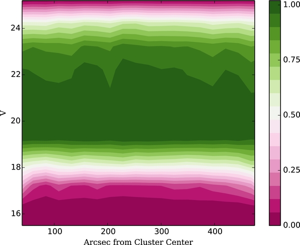
Figure 2. Completeness as a function of radius from the cluster center and magnitude for Ko 2. On the y-axis, bright magnitudes are incomplete due to image saturation and completeness quickly drops at faint magnitudes. There is very little trend in distance on the x-axis, as even the cluster center is relatively uncrowded.
Download figure:
Standard image High-resolution imageUsing the stellar weights, we made accurate measurements of the positions and profiles of the two clusters. Figure 3 shows the location of the stars in Ko 1. The cluster center is R.A.  and decl.
  . The cluster appears to have a clear edge at a radius of approximately 1.5 arcmin. Figure 4 shows the location of stars in Ko 2. The center of Ko 2 is R.A.
  and decl.
  . The cluster density drops off rapidly and the cluster appears to be truncated at a radius of 1.0 arcmin. Properties of the two clusters can be seen in Table 2.

Figure 3. Stellar density for all stars detected near Ko 1. The gap in the center of the cluster is caused by the bright saturated star aligned with the cluster. White represents the highest density regions.
Download figure:
Standard image High-resolution image
Figure 4. Stellar density for all stars detected near Ko 2.
Download figure:
Standard image High-resolution imageTable 2. Cluster Properties
| Ko 1 | Ko 2 | |
|---|---|---|
| R.A. (J2000) |  |
 |
| Decl. (J2000) |  |
 |
| l |  |
 |
| b |  |
 |
| (m − M) | 17.8 | 17.75 |
| R☉ | 34.9 ± 1.6 kpc | 33.3 ± 1.5 kpc |
| RGC | 36.3 ± 1.7 kpc | 26.3 ± 1.2 kpc |
| rα | 1 5 5 |
10 |
| rcluster | 15.8 pc | 9.6 pc |
| Mtot, V | 2.01 | 0.03 |
Download table as: ASCIITypeset image
4. CMDs, LFs, AND ANALYSIS
Isochrone fitting of cluster CMDs typically involves four free parameters: distance modulus, color excess, age, and metallicity. The distance modulus shifts the isochrone up and down relative to the data while the color excess shifts the isochrone left and right. Increasing age and metallicity are degenerate; both changes move the isochrone diagonally to the lower right. In the cases of Ko 1 and Ko 2, previous work on the clusters provides no constraints on any of the four parameters. Instead, we have drawn on a wide variety of external sources to constrain the fits. We have taken the color excess constraint from Schlegel et al. (1998) and Schlafly & Finkbeiner (2011), which suggest that both clusters are largely unreddened. Schlafly & Finkbeiner (2011) gives a E(V − I) color excess of 0.03 for Ko 1 and 0.049 for Ko 2. The Schlegel et al. (1998) color excesses are 0.034 for Ko 1 and 0.054 for Ko 2. Given the small difference, we adopt the well-tested Schlegel et al. (1998) values.
Metallicity is one of the hardest parameters to deal with; conventionally, isochrone fitting is completed after metallicity is determined spectroscopically. However, with no red giant branch (RGB) stars and a main sequence turnoff (MSTO) around V = 21, spectroscopy of the stars in Ko 1 and Ko 2 is prohibitively difficult to obtain. Instead, we determined cluster metallicity though a secondary method. The slopes of the RGB and, to a lesser degree, the main sequence (MS) are functions of metallicity, with the tip of the RGB and the lower MS stretching farther to the red as metallicity increases. We use this realization with a bootstrap method to determine the metallicity of Ko 1 and Ko 2, matching their CMDs to a CMD with a similar age and a known metallicity. In Figures 5 and 6, we show the CMDs for Ko 1 and Ko 2 overplotted on Figure 1(d), showing the CMD of M54 and the Sag dwarf from Siegel et al. (2007). We used the Sirianni et al. (2005) prescription to transform the data from the HST/ACS F606W and F814W bandpasses to V and I. The Ko 1 and Ko 2 CMDs were then reddened and shifted in magnitude to match the extinction and distance modulus of the intermediate population identified in the other work. While the small populations of Ko 1 and Ko 2 add some complexity to the analysis, the CMDs agree very well with intermediate populations in the Siegel et al. (2007) work. Thus, we adopt a metallicity of [Fe/H] = − 0.60 based on the MS agreement and take the age range of 4–6 Gyr as a likely match for Ko 1 and Ko 2.
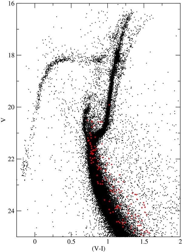
Figure 5. CMD for M54 and the Sag dwarf from Siegel et al. (2007) overplotted with the Ko 1 CMD. There is good agreement between the Ko 1 CMD and the [Fe/H] = −0.60 population identified in the other work.
Download figure:
Standard image High-resolution image
Figure 6. CMD for M54 and the Sag dwarf from Siegel et al. (2007) overplotted with the Ko 2 CMD. There is good agreement between the Ko 2 CMD and the [Fe/H] = −0.60 population identified in the other work.
Download figure:
Standard image High-resolution imageIn the previous work on these clusters, Koposov et al. (2007) used low-metallicity isochrones with [Fe/H] = −2.0. This decision was apparently based on the assumption that Ko 1 and Ko 2 have enrichments similar to the old halo globular clusters. This resulted in very poor isochrone fits in that work with isochrones that are far bluer than the stellar data on the MS.
With metallicity and color excess determined, we used Dartmouth Stellar Evolution Program (DSEP; Dotter et al. 2007) isochrones to determine cluster ages. Age and distance modulus were determined using the classical method of matching the magnitude of the MS and color of the MSTO. Using this method, age can be determined with an uncertainty of approximately 1 Gyr and the distance modulus to within 0.1 mag. The isochrone fits can be seen in Figures 7 and 8. For both clusters, we used isochrones with [Fe/H] = −0.60 and [α/Fe] = +0.20. From the fits, we find an age of 7 Gyr and a distance modulus of 17.8 mag for Ko 1 and an age of 5 Gyr and a distance modulus of 17.75 mag for Ko 2. Due to the difficulties stemming from the small population of stars in each cluster, these ages have uncertainties of approximately 1 Gyr and the distance moduli are uncertain at approximately the 0.1 mag level. Decreasing the metallicity by 0.1 dex results in ages approximately 1 Gyr younger and distance moduli 0.1 mag closer.
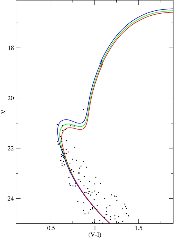
Figure 7. CMD for stars within 1.5 arcmin of Ko 1. The green (solid) line is a 7 Gyr DSEP isochrone with [Fe/H] = −0.60, [α/Fe] = +0.20 at (m − M) = 17.8, and E(V − I) = 0.034. The blue (dotted) and red (dashed) lines are similar isochrones with ages of 6 and 8 Gyr, respectively.
Download figure:
Standard image High-resolution image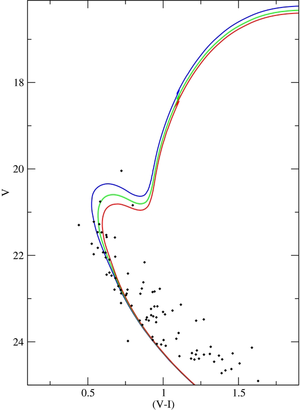
Figure 8. CMD for stars within 1.0 arcmin of Ko 2. The green (solid) line is a DSEP isochrone with an age of 5 Gyr and [Fe/H] = −0.60, [α/Fe] = +0.20 at (m − M) = 17.75, and E(V − I) = 0.054. The blue (dotted) and red (dashed) lines are similar isochrones with ages of 4 and 6 Gyr.
Download figure:
Standard image High-resolution imageWe have created completeness-correct stellar LFs covering the cluster MSs. Two criteria were used to select stars for creation of the LFs. First, spatially, the stars must be within the cluster radius. Second, in color–magnitude space, the stars could not be bluer than 2σ(V − I) of the MS nor redder than approximately 2σ(V − I) of the equal-mass binary sequence. The selected stars were then weighted by the inverse of their completeness value and the weights were summed in 0.5 mag bins. Due to the depth of the photometry, the LFs are sensitive to the underlying present-day mass functions (PDMFs) of the clusters. This sensitivity makes it possible to test the hypothesis that Ko 1 and Ko 2 are heavily stripped GCs.
It is helpful to examine the evolution of cluster MFs due to tidal stripping. This can be examined in three ways: analytically, numerically, and observationally. Analytically, Gunn & Griffin (1979) show that the radial density distribution for a minor component in an isothermal model is ρ(m) ∝ r−α with α = 2m/M, where m is the mass of the minor component and M is the mass of the major component. In a given annulus, then, the full range of stellar masses in the cluster will be present, with the mass distribution being a power law. As this annulus moves outward, the population will become more and more dominated by lower-mass components. This is a simple statement of mass segregation in clusters. When the cluster is then truncated by tidal forces at some radius, Rtrunc, the cluster will lose stars of all masses but with a probability of loss proportional to m−1. Assuming the cluster started with a power-law MF, this mass loss will maintain the power law shape but shift the slope from the slope of the initial mass function (IMF) to one that is shallower. Numerically, the n-body simulations of Lamers et al. (2013) show the same result. Initially, before the cluster experiences mass segregation, mass loss from the cluster does not change the slope of the PDMF. As time passes, the cluster becomes mass segregated. In this situation, mass loss causes the PDMF of the MS to decreases in slope until the PDMF eventually becomes dominated by stars near the MSTO. However, even after extreme mass loss, the PDMF remains a power law with constant slope from the MSTO to the lowest masses. Observationally, this same result is seen in the old globular clusters in Paust et al. (2010). The PDMFs become shallower and shallower in clusters with more mass loss, but they remain power laws with constant slope. As a result, we can use a cluster PDMF to diagnose the mass loss history. Heavily stripped clusters will have flat PDMFs or even positively sloped PDMFs, while unstripped clusters should have PDMFs that match the Salpeter IMF. This assumes a universal Salpeter IMF, as suggested by Elmegreen (2009).
To investigate the PDMFs of Ko 1 and Ko 2, we have produced the PDMFs seen in Figure 9 for Ko 1 and Figure 10 for Ko 2. To produce these PDMFs, DSEP models corresponding to the cluster ages and metallicities were used to translate the observed V magnitudes into stellar masses for each star. The stellar masses were then binned, accounting for completeness, to produce the PDMFs. For Ko 1, the bin size was 0.02 M☉. Ko 2 has fewer stars, and a bin size of 0.05 M☉ was used to ensure that each bin was reasonably populated. The small number of stars in each cluster causes large Poisson error bars and large uncertainties in the fit. The PDMF for Ko 1 has a slope of −2.27 ± 1.20 and the PDMF for Ko 2 has a slope of −2.20 ± 1.06. Despite the large uncertainties, we find central values very close to the Salpeter slope. These slopes are also approximately 2.5σ away from the measured slopes of known heavily stripped clusters such as NGC 6366 (Paust et al. 2009). It is important to note that these slopes are largely insensitive to our uncertainties in isochrone fitting. The DSEP mass–luminosity relationship for the best-fit isochrone to Ko 2 is shown in Figure 11. The section of the MS used to determine the cluster MFs is the extremely linear area from MV = 4 to 7. Model metallicity plays a very small role in the shape of this curve; indeed, changing from [Fe/H] = − 0.60 to −0.50 maintains exactly the same shape as the MLR curve but increases the mass at a given magnitude by 0.02 M☉. This will slightly shift the masses in the PDMF but will leave the slope unchanged. Similarly, any reasonable uncertainties in age and distance modulus from isochrone fitting may lead to a small shift in mass (again, on the order of two one hundredths of a solar mass) but it will not change the slope of the derived PDMF.

Figure 9. PDMF for Ko 1. The data points and error bars represent mass bins below the MSTO of Ko 1 on the MS. Fitting a line to the points results in a slope of −2.27 ± 1.20.
Download figure:
Standard image High-resolution image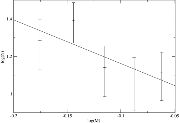
Figure 10. PDMF for Ko 2. The data points and error bars represent mass bins below the MSTO of Ko 2 on the MS. Fitting a line to the points results in a slope of −2.20 ± 1.06.
Download figure:
Standard image High-resolution image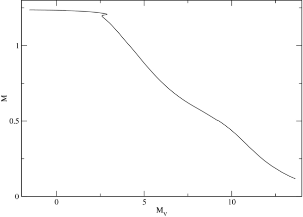
Figure 11. DSEP mass–luminosity relationship (MLR) for a 4 Gyr, [Fe/H] = − 0.60, [α/Fe] = 0.20 population to match Ko 2. The MLR for models matching Ko 1 is obviously the same, although the older age results in a lower maximum mass. The main sequences of Ko 1 and Ko 2 fall on the linear region from MV = 4 to 6.
Download figure:
Standard image High-resolution imageWe provide a sanity check for the PDMF fits by directly comparing the observed LFs for the two clusters to theoretical LFs. The LF of Ko 1 is seen in Figure 12 and enumerated in Table 3. As can be seen from Figure 12, the PDMF appears to match the Salpeter IMF very well, as expected. Examining the eight bins of the LF that comprise the MS, we examine the goodness of fit using the reduced-χ2 statistic. For the Salpeter slope LF,  . This statistic is worse for the other models with
  for the α = −3.00 model and
  for the α = −1.00 model. Thus, the deviations between the observed and theoretical LFs are nearly exactly as expected, given the uncertainties, for the Salpeter slope model and worse for the other two models. Following the suggestions of Andrae et al. (2010), we examine the residuals between the observed and theoretical LFs and find a similar result. The standard deviations of the residuals are 0.95, 1.09, and 1.25 for the α = −2.35, −3.00, and −1.00 models. Close agreement between the observed and theoretical LFs should result in a standard deviation of 1.0. Similarly, the LF of Ko 2 is seen in Figure 13 and Table 4. As can be seen in Figure 13, the LF of Ko 2 matches a theoretical LF with a Salpeter IMF even better than the LF of Ko 1. Unfortunately, the large Poisson errors caused by the small number of stars in the cluster complicate the statistical analysis of the fit. For the Salpeter slope,
  . It is 50% worse for the α = −3.00 model at
  and five times worse for the α = −1.00 model at
  . The residuals are distributed with standard deviations of 0.38, 0.48, and 0.89 for the α = −2.35, −3.00, and −1.00 models. While all of the theoretical models "overfit" the data, the Salpeter slope model is the best fit.
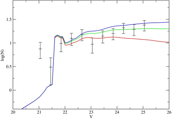
Figure 12. V LF for Ko 1. The lines shown are DSEP 7 Gyr LFs with [Fe/H] = −0.60 and [α/Fe] = +0.2 at (m − M) = 17.8 normalized to the observed LF. The theoretical LFs have α = −3.00, α = −2.35 (Salpeter), and α = −1.00 for the blue (dotted), green (solid), and red (dashed) lines, respectively.
Download figure:
Standard image High-resolution image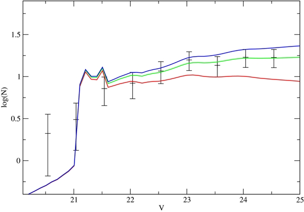
Figure 13. V LF for Ko 2. The lines shown are DSEP 5 Gyr LFs with [Fe/H] = −0.60 and [α/Fe] = +0.2 at (m − M) = 17.75 normalized to the observed LF. The theoretical LFs have α = −3.00, α = −2.35 (Salpeter), and α = −1.00 for the blue (dotted), green (solid), and red (dashed) lines, respectively. The data points on the MS agree perfectly with a DSEP luminosity function with a Salpeter slope.
Download figure:
Standard image High-resolution imageTable 3. Ko 1 V LF
| V | N | CN | Comp. | Log(CN) | Log(CN + σ) | Log(CN − σ) |
|---|---|---|---|---|---|---|
| 21.05 | 7 | 7.48 | 0.94 | 0.874 | 1.013 | 0.668 |
| 21.45 | 3 | 3.08 | 0.98 | 0.488 | 0.686 | 0.114 |
| 21.85 | 9 | 9.77 | 0.92 | 0.990 | 1.115 | 0.814 |
| 22.25 | 12 | 12.47 | 0.96 | 1.096 | 1.206 | 0.948 |
| 22.65 | 14 | 15.16 | 0.92 | 1.181 | 1.284 | 1.046 |
| 23.05 | 8 | 9.41 | 0.85 | 0.947 | 1.105 | 0.784 |
| 23.45 | 12 | 14.00 | 0.86 | 1.146 | 1.156 | 0.998 |
| 23.85 | 14 | 15.91 | 0.88 | 1.202 | 1.303 | 1.067 |
| 24.25 | 17 | 20.94 | 0.81 | 1.321 | 1.415 | 1.200 |
| 24.65 | 14 | 19.43 | 0.72 | 1.288 | 1.391 | 1.153 |
| 25.05 | 16 | 23.90 | 0.67 | 1.378 | 1.475 | 1.254 |
Notes. V is the magnitude at the center of the magnitude bin. N is the raw number of stars counted per bin. CN is the corrected number including completeness. Comp. is the average completeness of the stars per bin. The remaining three columns are the log of the corrected number and the logs of the 1σ error bars.
Download table as: ASCIITypeset image
Table 4. Ko 2 V LF
| V | N | CN | Comp. | Log(CN) | Log(CN + σ) | Log(CN − σ) |
|---|---|---|---|---|---|---|
| 21.04 | 3 | 3.08 | 0.97 | 0.489 | 0.686 | 0.115 |
| 21.54 | 7 | 7.20 | 0.97 | 0.857 | 0.997 | 0.732 |
| 22.04 | 8 | 8.34 | 0.95 | 0.921 | 1.053 | 0.732 |
| 22.54 | 11 | 11.64 | 0.94 | 1.066 | 1.180 | 0.910 |
| 23.04 | 14 | 15.76 | 0.89 | 1.198 | 1.300 | 1.063 |
| 23.54 | 11 | 13.60 | 0.81 | 1.134 | 1.248 | 0.978 |
| 24.04 | 12 | 16.96 | 0.71 | 1.229 | 1.340 | 1.081 |
| 24.54 | 10 | 16.88 | 0.59 | 1.227 | 1.347 | 1.062 |
Note. For a description of the columns, see the notes of Table 3.
Download table as: ASCIITypeset image
Works such as Kruijssen (2009) have shown that the PDMF of clusters can become curved rather than follow a straight power law. This occurs because encounters between stars with large differences in mass transfer the most energy. In a mass segregated cluster, the high-mass stars are locked deep in the cluster core and these interactions become rare. The existence of this curvature could raise doubts that the PDMFs measured for Ko 1 and Ko 2 represent the true PDMF below the limiting magnitude of this work. However, Lamers et al. (2013) shows that this curvature does not become significant until a significant amount (∼70%) of the cluster mass has been lost. At that point, clusters appear to have flat PDMF slopes, in stark contrast to the steep PDMF slopes of Ko 1 and Ko 2. As a result, we conclude that the measured PDMF for both clusters maintains a constant slope to lower magnitudes.
Koposov et al. (2007) classified Ko 1 and Ko 2 as globular clusters based on appearance, thinking they looked like heavily stripped globular clusters. However, the degree of mass loss required to transform even a small globular cluster into an object the size of Ko 1 or Ko 2 would result in a flat PDMF. The new analysis of the PDMF illuminates the fact that Ko 1 and Ko 2 have always been small clusters and have not lost significant amounts of mass. It is therefore reasonable to reclassify them, based on their size, as open clusters.
Using the completeness-corrected LFs, we can determine the integrated magnitude of the clusters by summing the magnitudes of stars in each bin. While this includes only the top three magnitudes of the MS, stars farther down the MS contribute an insignificant amount of light. We have assumed that the small number of bright stars in the RGB portion of the LF are actually foreground stars and not cluster members. Simple magnitude addition results in mV = 19.83 for Ko 1. Using the extinction from Schlafly & Finkbeiner (2011) and the fit distance modulus, the integrated absolute magnitude is MV = 2.01. Ko 2 has mV = 17.76 and, correcting for extinction, MV = 0.03. These results are several magnitudes fainter than the previously discovered satellite galaxies and GGCs. Indeed, Segue 1, a heavily stripped globular cluster, has MV = −3.0 (Belokurov et al. 2007).
By summing and extrapolating data from the LF, we can confirm the stability of the clusters. The Ko 2 MSTO occurs at approximately M = 1.2 M☉ and the faint magnitude limit corresponds to M = 0.7 M☉ stars. Assuming a Salpeter MF slope, the observed magnitude range represents only 1/35 of the stars in the cluster. The observed 87 stars therefore indicate a total stellar population of approximately 3,000 stars. Assuming an average stellar mass of 0.6 M☉, the cluster has a total mass of 1800 M☉. We have used a simple relationship for tidal radius, rt = RGC(2(MCL/MG))1/3 (von Hoerner 1957), and assumed that clusters fill their tidal radii at any distance (Webb et al. 2013). This simplifies the analysis since no assumed orbit or perigalactic distance is required. With these assumptions, we calculate rt = 45 pc for Ko 2 and rt = 115 pc for Ko 1. As both clusters have tidal radii many times larger than their physical extents, both clusters are stable against tidal stripping. Indeed, Ko 1 would have to come within approximately 4.9 kpc of the GC for the tidal radius to shrink to match the cluster diameter. For Ko 2, this distance is 5.5 kpc.
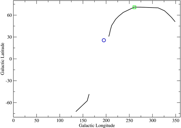
One hint as to the origins of these clusters comes from recent maps of the Sag stream in Newby et al. (2013). As seen in Figure 14, both clusters fall on or in close proximity to the Sag stream. Ko 1 is only 0.2 degrees in l and 0.3 degrees in b from the stream center, which is small compared to the approximately three degree width of the stream at that position. The galactocentric distance for the stream at the position of Ko 1 is 27.0 ± 8.0 kpc, agreeing at the 1σ level with the galactocentric radius of 36.3 ± 1.7 kpc for Ko 1. Ko 2, unfortunately, lies at the very edge of the SDSS footprint. This prevented Newby et al. (2013) from tracing the stream to the location of Ko 2. At the nearest point in l and b, however, the stream is several degrees wide and has a distance of 17 ± 18 kpc from the galactic center, comparable to the 26.3 ± 1.2 kpc distance we find for Ko 2. These galactocentric distances assume a 8.5 kpc separation between the galactic center and the Sun. Given the path of the Sag stream, it is unlikely that the clusters have ever experienced such a strong tidal field.
Figure 14. Positions of the Sagittarius stream centers from Newby et al. (2013). Ko 1 is represented by the square and Ko 2 by the circle.
Download figure:
Standard image High-resolution image
5. CONCLUSIONS
We have performed an in-depth investigation of the Galactic star clusters Ko 1 and Ko 2 with DCT/LMI photometry, observing several magnitudes deeper than the previous study of Koposov et al. (2007). Using this data, we have refined a number of the cluster parameters, cast serious doubts on the classification of Ko 1 and Ko 2 as stripped globular clusters, and provided hints as to the true nature of these clusters.
In summary, we have found the following.
1. Ko 1 has an age of 7 Gyr and Ko 2 has an age of 5 Gyr from isochrone fitting with DSEP isochrones (Dotter et al. 2007). These ages match the intermediate episodes of star formation in the Sagittarius dwarf (Siegel et al. 2007). The cluster metallicities also match metallicities seen in the Sagittarius dwarf.
2. Ko 1 is 34.9 kpc from the Sun and 36.3 kpc from the Galactic center. Ko 2 is 33.3 kpc from the Sun and 26.3 kpc from the Galactic center. This agrees well with the Galactocentric distance of the Sagittarius stream at the positions of the clusters (Newby et al. 2013).
3. The clusters have the lowest integrated magnitude of MW halo satellites with Mtot, V of 2.01 and 0.03 for Ko 1 and Ko 2, respectively. Despite their diminutive size, the clusters are currently stable against tidal stripping, due to their large distances from the Galactic center.
4. Analysis of the completeness-corrected PDMFs suggests that the clusters have not lost a significant amount of mass in their lifetimes. This conclusion comes from the extreme similarity between the slope of the PDMF and the slope of the Salpeter IMF. Mass loss from clusters flattens the PDMF slope, thus the match between the PDMF and IMF indicates that the clusters have not lost significant amounts of mass over their lifetimes.
5. Through these conclusions, we find that Ko 1 and Ko 2 are not GGCs, but rather open clusters removed whole from Sagittarius. To prove this conclusively, we require spectroscopic information to determine if the cluster velocities kinematically match the Sagittarius stream.
G.v.B. graciously acknowledges internal support from Lowell Observatory. Partial support of the DCT was provided by Discovery Communications. The LMI was funded by the National Science Foundation via grant AST-1005313.
Facility: DCT -