


ABSTRACT
Close-binary central stars of planetary nebulae (CSPNe) provide an opportunity to explore the evolution of PNe, their shaping, and the evolution of binary systems undergoing a common-envelope phase. Here, we present the results of time-resolved photometry of the binary central stars (CSs) of the PNe NGC 6026 and NGC 6337 as well as time-resolved spectroscopy of the CS of NGC 6026. The results of a period analysis give an orbital period of 0.528086(4) days for NGC 6026 and a photometric period of 0.1734742(5) days for NGC 6337. In the case of NGC 6337, it appears that the photometric period reflects the orbital period and that the variability is the result of the irradiated hemisphere of a cool companion. The inclination of the thin PN ring is nearly face-on. Our modeled inclination range for the close central binary includes nearly face-on alignments and provides evidence for a direct binary-nebular shaping connection. For NGC 6026, however, the radial-velocity curve shows that the orbital period is twice the photometric period. In this case, the photometric variability is due to an ellipsoidal effect in which the CS nearly fills its Roche lobe and the companion is most likely a hot white dwarf. NGC 6026 then is the third PN with a confirmed central binary where the companion is compact. Based on the data and modeling using a Wilson–Devinney code, we discuss the physical parameters of the two systems and how they relate to the known sample of close-binary CSs, which comprise 15%–20% of all PNe.
Export citation and abstract BibTeX RIS
1. INTRODUCTION
The distinctly non-spherical shape of most planetary nebulae (PNe) indicates the presence of a shaping mechanism which is not presently understood. The interacting stellar winds model of Kwok et al. (1978) and the generalized interacting stellar winds model (e.g., Balick 1987; Balick & Frank 2002) have proven effective in describing many of the global shapes seen in PNe. In these models, a slow, thick wind blows during the upper asymptotic giant branch (AGB) reducing the envelope mass, followed by a fast, tenuous wind, from the contracting and heating post-AGB star. However, to recreate PN shapes, the slow AGB wind is assumed to be equatorially enhanced. Additional features such as jets, ansae, and other point symmetries have been explained by assuming that the fast wind is highly collimated (Sahai & Trauger 1998), but the physical mechanisms behind the collimation are also not explained. Several theories exist which attempt to explain the underlying mechanism(s) responsible for shaping. Two classes of mechanism are widely invoked: binarity (e.g., Bond & Livio 1990; Yungelson et al. 1993; Soker 1997; Bond 2000; Zijlstra 2007; De Marco 2009) or single stars with particular ranges of progenitor mass resulting in high stellar rotation and magnetic fields (e.g., Stanghellini et al. 1993; Corradi & Schwarz 1995; Zhang & Kwok 1998; García-Segura et al. 1999, 2005). However, Soker (2006) and Nordhaus et al. (2007) showed that magnetic fields in single AGB stars cannot be easily sustained for longer than about 100 years because their action feeds back on the stellar differential rotation that generates them in the first place. As a result of these theoretical results, the binary hypothesis has gained momentum.
In this series of papers, we examine the binary shaping mechanism in light of the observational evidence, specifically for close-binary central stars of planetary nebulae (CSPNe). In De Marco et al. (2008, hereafter Paper I), we reviewed the status of our knowledge of post-common-envelope binary CSs (but see also De Marco 2009, where additional binaries found by Miszalski et al. 2009a were listed), emphasizing their relation to other CSs.
From binary population synthesis calculations by, e.g., Yungelson et al. (1993) and Willems & Kolb (2004), it is apparent that close stellar companions undergoing a common-envelope (CE) interaction on the AGB should result in a significant fraction of PN surrounding central binaries with orbital periods shorter than a few days. Photometric variability may occur in close-binary CSPNe through several mechanisms. For a mid- to late spectral type companion, the systems should exhibit variability due to the irradiated inner hemisphere of the companion. If the binary orbital inclination is near 90°, eclipses may be observed. Or if one of the components fills a large fraction of its Roche lobe, the deformation of the stellar surface will cause photometric variability with two cycles per orbital period (ellipsoidal variability).
To date 35 CSPNe have been identified in the literature as close binaries which show variability from irradiation effects, eclipses, ellipsoidal effects, or a combination thereof. Two additional systems do not show photometric variability but have been identified as spectroscopic binaries. The currently identified close-binary CSs are summarized in Paper I, Miszalski et al. (2009a, 2009b), and De Marco (2009). Paper I reviewed the then-known binary CSPNe, the number of which were more than doubled by Miszalski et al. (2009a). Their follow-up paper (Miszalski et al. 2009b) along with the review of De Marco (2009) describes the current statistics of binary CSPNe and the state of the PN shaping debate. Of the 35 photometrically variable binary CSs, only two have orbital periods greater than 3 days (PN G355.6-02.3 and PN G001.8-03.7). One other PN, SuWt 2, has a reported binary with period greater than 3 days, but this likely does not include the CS (Paper I; Bond et. al 2008). The majority of these systems do not have spectroscopic data and a number do not even have published light curves (we have observed these systems and will provide light curves in a later paper in this series). Bond (2000) gives the empirical fraction of detectable close binaries as ∼10%–15% and Miszalski et al. (2009a) as ∼12%–21%. The discovery of the binarity of the CSs of NGC 6026 and NGC 6337 was presented by Hillwig (2004) in a photometric study of a group of CSs classified by Soker (1997) as likely having main-sequence companions which underwent a CE phase. The study was biased toward finding binary CSPNe and resulted in a binary fraction of 25%, though due to the small sample size (eight), it is impossible to make any clear conclusions about binary fraction.
Understanding the relation between binarity and the PN phase is an important and active field of study at this time. The PlaN-B working group6 has been established as a means of combining diverse observational and theoretical approaches to the problem. Several methods may be used to observationally test the binarity-PN relationship. The presence of close-binary stars in PNe of specific morphology can be found with a statistically significant sample of close-binary CSPNe. The number of known systems is gradually reaching this level. In addition, physical parameters of the binary systems such as inclinations derived from binary system modeling will allow comparison of the binary orbital axis with the major axis (or axes) of the surrounding PN. Other binary parameters (e.g., double versus single degenerate systems) may also be compared to nebular morphology in a search for correlated parameters. Being able to identify He white dwarfs (WDs) will allow a test of CE evolution theory and its application to the ejection of PNe by comparing post-AGB to post-red giant branch (RGB) evolution. And the fraction of double degenerates versus single degenerate systems may be compared to predictions of CE and population synthesis models.
2. OBSERVATIONS AND REDUCTIONS
2.1. Photometry
The photometric data consist of V-band CCD photometry obtained at the SMARTS 0.9 m telescope7 located at Cerro Tololo Inter-American Observatory (CTIO) with the T2K Imager and B-, V-, and R-band photometry obtained at the CTIO 1.0 m telescope with the SITe SI-502A 512 × 512 pixel CCD imager.
The exposures were reduced with aperture photometry using the DAOPHOT package of IRAF8 to produce raw photometry which was then analyzed by incomplete ensemble photometry (Honeycutt 1992). The results are instrumental magnitudes dependent on the instrumental response of the CTIO 0.9 m and 1.0 m systems and on the full ensemble of stars used in the solution for each target (>100 stars in each case). The zero point used is not calibrated to the standard BVR system. The average systematic errors typically fall between ∼0.001 and ∼0.005 mag. No attempts were made to remove nebular contamination beyond typical background subtraction. However, we did thoroughly examine the data for trends relating to changes in seeing and airmass. No dependence was found related to these values for either CS.
Tables 1 and 2 give the instrumental magnitudes for the CSs of NGC 6026 and NGC 6337, respectively (see the electronic version for the full tables). The tables include the photometry presented in Hillwig (2004), reanalyzed with the new data.
Table 1. Instrumental Magnitudes of the Central Star of NGC 6026
| HJD | Binstr | σB | HJD | Vinstr | σV | HJD | Rinstr | σR |
|---|---|---|---|---|---|---|---|---|
| (2,450,000) | (mag) | (mag) | (2,450,000) | (mag) | (mag) | (2,450,000) | (mag) | (mag) |
| 3476.79213 | 10.290 | 0.002 | 2395.79584 | 9.366 | 0.001 | 3476.79495 | 9.872 | 0.001 |
| 3476.79647 | 10.284 | 0.003 | 2395.79012 | 9.380 | 0.001 | 3476.79930 | 9.862 | 0.001 |
| 3476.80082 | 10.275 | 0.002 | 2395.79321 | 9.373 | 0.001 | 3476.80365 | 9.858 | 0.001 |
Only a portion of this table is shown here to demonstrate its form and content. Machine-readable and Virtual Observatory (VO) versions of the full table are available.
Download table as: Machine-readable (MRT)Virtual Observatory (VOT)Typeset image
Table 2. Instrumental Magnitudes of the Central Star of NGC 6337
| HJD | Binstr | σB | HJD | Vinstr | σV | HJD | Rinstr | σR |
|---|---|---|---|---|---|---|---|---|
| (2,450,000) | (mag) | (mag) | (2,450,000) | (mag) | (mag) | (2,450,000) | (mag) | (mag) |
| 3477.79437 | 12.972 | 0.003 | 2395.88904 | 11.833 | 0.002 | 3477.80332 | 12.196 | 0.003 |
| 3477.80804 | 12.889 | 0.003 | 2395.89517 | 11.835 | 0.002 | 3477.81700 | 12.109 | 0.003 |
| 3477.82262 | 12.795 | 0.003 | 2395.89966 | 11.856 | 0.002 | 3477.83157 | 12.068 | 0.003 |
Only a portion of this table is shown here to demonstrate its form and content. Machine-readable and Virtual Observatory (VO) versions of the full table are available.
Download table as: Machine-readable (MRT)Virtual Observatory (VOT)Typeset image
2.2. Spectroscopy
Spectroscopy of NGC 6026 was obtained at the SMARTS 1.5 m telescope7 located at CTIO using the 831 lines/mm grating in second order with a range 4067–4749 Å with a 3 6 slit. The resulting resolution was ≈1.2 Å at the central wavelength. The spectra were reduced using the DOSLIT package in IRAF. A HeAr lamp was used to wavelength calibrate the spectra. The resulting calibration error was generally <0.01 Å. The spectra were then continuum normalized to a value of unity. Radial velocities were obtained through cross-correlation function (CCF) fitting. Initially, the first spectrum was used as a template. The hydrogen and He ii λ4686 lines were not used due to the strong PN emission filling in the absorption lines. Other spectral regions which showed either emission from the PN or interstellar features (such as the strong diffuse interstellar band near 4430 Å) were also excluded from the fitting. Once initial velocities were found, all spectra were shifted to a common reference frame and co-added. The co-added spectrum was then used in a second CCF fitting iteration to provide more accurate radial velocities. These velocities were used to shift and co-add the spectra to provide a final high signal-to-noise ratio spectrum of NGC 6026. The final co-added spectrum is shown in Figure 1.
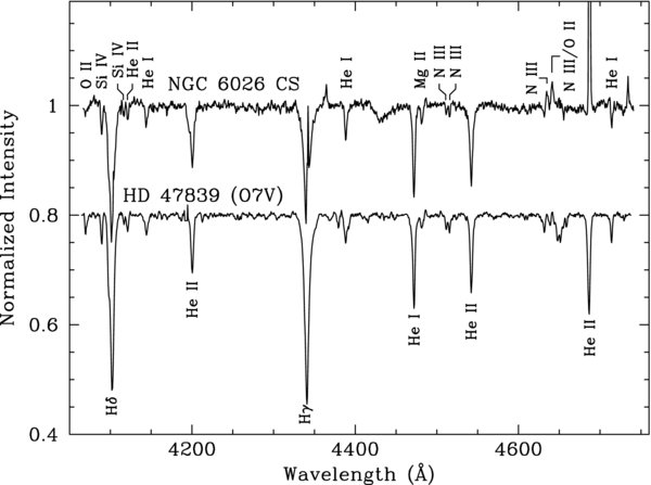
Figure 1. Continuum normalized spectrum of NGC 6026 consisting of the phase shifted and co-added individual spectra. Also shown is the O7 V star HD 47839, normalized and shifted downward by 0.2 units for clarity.
Download figure:
Standard image High-resolution image3. ANALYSIS
3.1. NGC 6026
3.1.1. Background and Data Analysis
The PN NGC 6026 has a lopsided appearance in images taken with short exposure times (see Figure 2). However, deep exposures reveal a symmetric elliptical morphology. Frew (2008) gives a nebular age of 6 × 10³ years and CS temperature of >35,000 K. Stanghellini et al. (1993) give a Zanstra temperature for the CS of 68,000 K and Grewing & Neri (1990) give a temperature of 26,000 K from UV color indices.
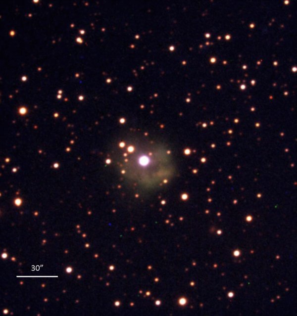
Figure 2. Color composite image of NGC 6026 created using co-added B, V, and R images from the CTIO 0.9 m telescope. North is up and east is left.
Download figure:
Standard image High-resolution imageThe original photometric data in Hillwig (2004) were fit using a sine curve resulting in a period with a value half that of the eventually determined orbital period. The new V-band light curve of NGC 6026 folded on this period shows obvious departure from a sine curve as well as significant scatter at minimum and maximum. The solution to these issues is found in the radial-velocity data which show a period of twice that found originally from photometry. The radial-velocity data were used in periodogram, a program which uses the period search technique of Scargle (1982) as modified by Horne & Baliunas (1986). The highest peak is located at P = 0.528 days.
Radial velocities obtained from the spectra as described above were used with the multi-epoch light curve data to determine a more accurate ephemeris. The derived ephemeris for NGC 6026 is

which is in the form T = T0 + Porb × E, where T gives the HJD of orbital phase zero (taken to occur at superior conjunction of the CS) and E is the number of elapsed cycles since T0. Figures 3 and 4 show the radial-velocity data and light curves folded on the ephemeris given above. The fit lines in both figures are from the Wilson–Devinney modeling described below for  , where M2 is the mass of the companion and
  is the mass of the CS.
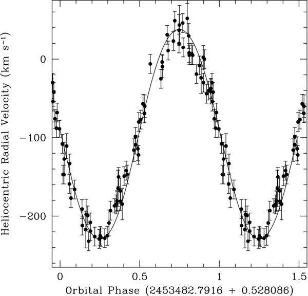
Figure 3. Phase-folded radial-velocity curve of NGC 6026 for the period given in the ephemeris (Equation (1)). The fit line is from the Wilson–Devinney model described in Section 3.1.2. We find a system velocity of γ = −93.4 km s−1 with a radial-velocity amplitude for the CS of  km s−1.
Download figure:
Standard image High-resolution imageFolded on the spectroscopic orbital period, the light curve of NGC 6026 (see Figure 4) shows two photometric maxima per orbit, suggesting that the photometric variation is caused by ellipsoidal variability. The two-cycle-per-orbit light curve and the low amplitude of the variability also indicate that the irradiation effect is not strong. If an irradiation effect is present in a light curve dominated by ellipsoidal variability, it would create unequal depths in the two minima. Minima depths are also affected by the difference in gravity darkening between the inner hemisphere (near the L1 point) and outer hemisphere. In the case of irradiation in an ellipsoidal variability dominated system, the depths of the two minima are then dependent upon both any irradiation effect and gravity darkening in the atmosphere.
We do find deviations in the light curve that do not show periodic behavior. In particular, we see in our phase-folded light curve from phase 0.2–0.4 the 2005 April 17 data are approximately 0.03 mag fainter than overlapping photometry from nights in 2002, 2004, and 2005. The total extent of the data from 2005 April 17 is from about phase 0.9–0.4. Between phases 0.9 and 0.2, the photometry agrees with the rest of the data.
Two other locations in which the light curve appears inconsistent are just after phase 0.6, where data from 2002 April 30 are also approximately 0.03 mag fainter than the remainder of the data. Also, around phase 0.8, data from 2005 April 15 show a similar drop, though in this case lasting for less 10% of the phase. Both before and after, the data correspond to that from the other nights.
There is no immediately recognizable instrumental or atmospheric cause for these drops in brightness. The seeing, transparency, and focus are all stable and the airmass does not drop to unreasonable values (nor would it be expected to cause a fast drop to values that are consistently fainter than the unaffected data for up to 2.5 hr). This suggests that the drop may be intrinsic to the system. In such a case, intervening knots of dust in the surrounding nebulosity are one possible cause. The relatively broad emission lines of N iii and O ii near λ4640 and He ii λ4686 (see Figure 1) are reminiscent of wind emission observed in Of-type stars. However, the gradient in intensity of the nebula at the location of the CS (see Figure 2) makes complete nebular subtraction difficult. Therefore, the He ii λ4686 and Hγ λ4340 lines also include emission due to incomplete subtraction of the nebular spectrum. The N iii and O ii lines near λ4640 also show variable line strength and velocities that do not appear to be associated with the orbital period. The variability also suggests that these lines may originate in a wind, similar to colliding winds observed in other hot star binaries.
The fainter episodes are not just confined to the V-band data, but also appear in the B and R filters as well. Figure 4 shows the phase-folded light curves in all three filters. The B and R filters are more limited in data points because observations in these filters were only obtained during the 2005 observing run.
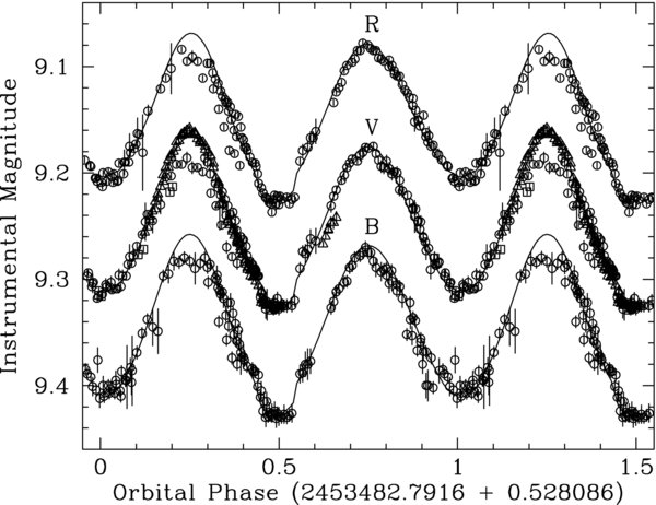
Figure 4. Phase-folded B-, V-, and R-band light curves of NGC 6026 for the period given in the ephemeris (Equation (1)). The curves have been vertically displaced from one another for clarity. The magnitude scale for the B light curve is used here with the R and V curves shifted, though keep in mind that the magnitudes are instrumental and so such shifts are not physically important. Data are from 2002 (triangles), 2004 (squares), and 2005 (circles). The fit lines are from the Wilson–Devinney model discussed in Section 3.1.2.
Download figure:
Standard image High-resolution imageThe CS spectrum, apart from emission filling in the Balmer and He ii λ4686 lines, is a good match to HD 47839 an O7 V star. A representative spectrum of HD 47839 is shown in Figure 1 with the CS spectrum. Comparing our spectrum to a tlusty model atmosphere grid (Hubeny & Lanz 1995) produces a good fit at T = 37,500 ± 2500 K and log g = 4.0 ± 0.2, based on the He i λ4471/He ii λ4541 line ratio as well as the wings of the Balmer lines in our spectral range. Our results agree well with the available literature values discussed above.
3.1.2. Wilson–Devinney Modeling
A Wilson–Devinney code (Wilson 1990; Wilson & Devinney 1971) was used with our photometric and radial-velocity data to find a best-fit solution for the system parameters. For this fitting, we omitted the points described above that fall below the majority of the data. Omitting these data includes the implicit assumption that these data are not representative of the true system brightness, which may or may not be correct. However, these points represent discrete drops in the light curve, so we have used the data which exhibit smooth, continuous light variations. The smoothly variable data allow the model fitting to provide a solution.
There are several observations that can be made to constrain the initial fit parameters. First, the period is quite well determined by the combination of three epochs of photometry and radial-velocity data scattered over roughly the same time period. Also, the fairly short orbital period places some limits on the physical size of both stars. The single-lined radial-velocity curve combined with the orbital period provides a direct relationship between the system mass ratio,  , and the average orbital separation, a. This comes about because the velocity amplitude for the visible CS combined with the orbital period provides a known value for the semimajor axis of the CS orbit,
  . Then, we have that
  . Likewise, the sum of the masses is related to P and a and thus to P and q. However, since q is the ratio of the masses, then a specific value of q results in unique values for
  and M2. For the purposes of our modeling, we will assume that any WD or pre-WD must have a mass that falls in the range 0.3 M☉ ⩽ M ⩽ 1.4 M☉.
Apart from the above parameters, we also make some specific deductions based upon the light curves. As mentioned previously, the double-peaked curves likely indicate an ellipsoidal effect and because we only see a single-lined spectrum, it is likely that the subdwarf CS nearly fills its Roche lobe. Also, due to the small radius required by the short orbital period, a main-sequence companion would be limited to the lower end of the mass range. The large temperature difference between the two components, combined with the large sizes of the stars relative to their separations, would result in a correspondingly large reflection effect. It would then be the reflection effect that would dominate the light curve.
The light curve also shows that the two maxima occur at different brightnesses. This only happens in ellipsoidal variability for a non-circular orbit. The calculated models show an eccentricity range of 0.010 and 0.025. Furthermore, a close inspection of Figure 4 shows that near phase 0.5 a clear discontinuity in the light curve is present that suggests an eclipse. The possible eclipse also appears to be nearly flat at mid-eclipse suggesting a totally eclipsing system. In fact, the orbital phasing we have used identifies this as an eclipse of the companion, not the CS. There is no clear eclipse of the CS at phase 0.0. Combining these two features suggests that the companion star is small (possible total eclipse, width of the eclipse, and no visible primary eclipse) and that the companion star is very hot (depth of the eclipse and no visible primary eclipse). The model suggests that the most likely companion to the CS is a hot WD or subdwarf. The best-fit model, shown in Table 3, results in a very high surface temperature for the companion. However, the temperature value is directly related to the stellar radius. The two parameters define the total luminosity of the star which directly impacts the amplitude of the variations as well as the depth of the observed eclipse. A small change in temperature requires a corresponding change in stellar diameter. Therefore, the two are strongly coupled in the model fitting. The flat eclipse removes the radius/temperature degeneracy, but only in the presence of a known mass ratio.
Table 3. Best-fit Model Physical Parameters for the CS of NGC 6026
| Parameter | Model Values | ||
|---|---|---|---|
| q | 0.63 | 1.0 | 1.35 |
| TCS (×103 K) | 22 | 38 ± 3 | 38 |
| T2 (×103 K) | 109 | 146 ± 15 | 146 |
| MCS (M☉) | 1.40 | 0.57 ± 0.05 | 0.30 |
| M2 (M☉) | 0.88 | 0.57 ± 0.05 | 0.41 |
| RCS (Pole, R☉) | 1.41 | 1.06 ± 0.05 | 0.78 |
| R2 (R☉) | 0.069 | 0.047 ± 0.005 | 0.043 |
 (cgs) (cgs) |
4.24 | 4.15 ± 0.02 | 4.08 |
 (cgs) (cgs) |
6.70 | 6.85 ± 0.05 | 6.78 |
| LCS (L☉) | 411 | 2070 ± 80 | 1121 |
| L2 (L☉) | 593 | 887 ± 40 | 742 |
| e | 0.010 | 0.025 ± 0.005 | 0.025 |
| ω (rad) | 3.84 | 3.84 ± 0.9 | 3.84 |
| i (deg) | 80 | 82 ± 2 | 84 |
| a (R☉) | 2.447 | 2.87 ± 0.10 | 3.618 |
Download table as: ASCIITypeset image
Using the mass limits for the subdwarf/WD companion described above, with the relationship between q and the masses, provides a mass ratio range of 0.63 ⩽ q ⩽ 1.35 and a corresponding range in CS mass of  M☉. Varying the mass ratio affects the stellar separation, a, the stellar radii, and to a lesser extent the surface gravities. For a given mass ratio, increasing the CS mass in turn directly affects the stellar separation, the required size of the CS (to achieve the ellipsoidal effect), and thus the required size (and temperature) of the companion. However, once again, the suspected eclipse provides some limits to these parameters. The relative stellar radii are constrained by three items: the width of the eclipse, the subdwarf's Roche lobe filling factor required for the ellipsoidal effect, and the relative amplitude of the eclipse and ellipsoidal effect. Putting all of this together means that for a given mass ratio, we derived reasonably constrained physical parameters for the system.
In Table 3, we show the results of our modeling for a mass ratio, q = 1. The errors given in the table represent the spread of values over which each variable still produces a good fit. We also show in the table the range for each value resulting from varying the mass ratio between the two limits discussed above. These ranges represent the possible values based on physical limits in the system. Mass ratios approaching the lower limit correspond to the largest component masses because the radial-velocity amplitude of the CS is set by the data. For the low q model the CS temperature is forced to values too low to be associated with our observed spectrum. To maintain a reasonable temperature for the CS, the mass ratio range can effectively be limited beyond that shown in Table 3, with an approximate lower limit of 0.8 M☉ ( and M2 ≈ 0.67). Furthermore, we may also expect that if the companion is more compact than the CS, then it is evolutionally more advanced than the CS. For a more evolutionary advanced state, it must have had a more massive progenitor and would likely have a more massive remnant. In this case, the mass ratio would be q ≳ 1.0. The modeled eccentricity, temperature, and inclination remain the same for mass ratios in the range 1.0 ≲ q ≲ 1.35. For values below q = 1.0, each of these physical parameters must be changed to result in a good fit to the data. The best-fit values shown in Table 3 correspond to the broadest mass ratio limits, q = 0.63 and q = 1.35. Also shown are model values for the likely lower limit of q = 1.00. We expect that the system parameters lie between the models for q = 1.00 and q = 1.35. Approximate uncertainties for individual parameters are given in the q = 1.00 model.
The range of values for the stellar diameter of the companion between 0.043 and 0.069 R☉ places it at more than twice the expected radius of an object supported by electron degeneracy pressure (see, e.g., Schmidt 1996). Both the larger than expected radius and high temperature of the companion may be due to accretion heating via a CE phase or an AGB/RGB wind. The accreted material may have created an expanded hot atmosphere. It does not seem likely that such an expanded atmosphere due to CE accretion would still be present given the approximate 6000 year age of the PN (Frew 2008) and the cooling rates for WDs in novae which occur on the scale of hundreds of years (Prialnik 1986). It is possible, given the non-cyclical variations seen in the light curve described above and the evidence in the spectrum for winds, that more recent wind accretion may be responsible for the increased size and temperature. It is unlikely that the faint, hot companion would be younger than the larger CS, given its much smaller size. It is possible that the companion has not yet contracted to the WD cooling track, which would require that the masses of the two progenitor stars were very nearly identical (the q = 1.0 model), which is statistically very unlikely.
We have used passband specific linear limb darkening coefficients from Van Hamme (1993) for the models. For the compact companion, the limb darkening coefficient used was 0.069 in all three filters. The CS coefficients used were 0.256 (B filter), 0.199 (V filter), and 0.095 (R filter). The final result is sensitive to the choice of limb darkening coefficient only for the CS and only for changes of the order of 20% or more in the coefficient value. Our values should be well within this uncertainty. In addition, given the high temperatures for both stars, we used an albedo of 1.0 for both components.
Comparing our temperature and log g values to the model atmosphere analysis of Napiwotzki (1999) in his Figure 2, we find that the CS of NGC 6026 falls very close to the evolutionary track for a 0.546 M☉ post-AGB star and a 0.414 M☉ post-RGB star. Our range in masses covers both of these values, so that we are unable to distinguish between a post-AGB versus post-RGB evolution for the CS based on the model results. However, the nebula is very highly ionized (de Vaucouleurs 1955), lacking [O ii] line emission and with strong He ii emission. The high ionization is inconsistent with the previously observed 35,000 K CS, but is more in line with the >109,000 K companion discussed above. It then appears that much of the ionization of the nebula is due to the compact, hot companion rather than the visible CS.
The modeled systemic velocity of the binary is γ = −93.4 ± 2.1 km s−1 which is consistent with the heliocentric radial-velocity for the PN in the literature of γ = −101.5 ± 4.7 km s−1(Durand et al. 1998).
3.2. NGC 6337
3.2.1. Background
NGC 6337 appears to be a nearly perfectly circular PN in most images (see Figure 5) and has been classified in most lists as round (or elliptical in the case where round nebulae are not classified separately). However, Corradi et al. (2000) and García-Díaz et al. (2009) have shown that the round nebulosity seen is the narrow waist of a nearly pole-on bipolar PN. The papers present deep images and spectra showing the edges of the polar lobes extending slightly outward from the bright ring in the northwest and southeast directions with detected polar caps. The nearly circular appearance of the bright ring suggests that the major axis of the nebula is tilted by ≲15° to our line of sight. The distinct appearance of the lobes on opposite sides of the ring, however, suggests that the tilt is likely closer to 15° than 0°. The true inclination though is difficult to extract without some knowledge of the axial ratio of the nebulosity, which can vary drastically among bipolar PNe.

Figure 5. Color composite image of NGC 6337 created using co-added B, V, and R images from the CTIO 0.9 m telescope. North is up and east is left.
Download figure:
Standard image High-resolution imageIt is also interesting to note that Corradi et al. (2000) and García-Díaz et al. (2009) also detect point-symmetric structures suggesting precessing outflows in their deep images of NGC 6337. The structures are reminiscent of similar features seen in the lobes of other bipolar PNe (e.g., Sahai 2004). Also seen in García-Díaz et al. (2009) and in our Figure 5 as the red filaments are features reminiscent of FLIERS (Balick et al. 1993).
In the case of NGC 6337, there are several published values for physical parameters of the nebula and CS. Regarding the temperature of the CS, the results of Gorny et al. (1997) and Stanghellini et al. (1993), 41,700 K and 44,870 K, respectively, are in good agreement and are both H i Zanstra temperatures. Amnuel et al. (1985), however, report a CS temperature of 105,000 K using nebular diameter and 5 GHz radio flux. The CS temperature is discussed below in the context of model fits to our data.
Gorny et al. (1997) present, in addition to CS temperature, estimates of the CS mass, evolutionary time of the nebula, and distance to the PN. Their distance, 1.6 kpc, agrees well with the published values of Acker et al. (1992, 1.1–1.7 kpc) and Stanghellini et al. (1993, 1.32 kpc). However, Frew (2008) gives a distance of 860 ± 200 pc. The CS mass of 0.563 M☉ given by Gorny et al. (1997) is consistent with their relatively low temperature. Evolutionary models then provide their reported evolutionary time of 2.42 × 10⁴ years. Frew (2008) reports an age of 1.2 × 10⁴ years derived from his surface brightness/radius relation. The major difference in nebular ages likely results from the author's different distance values.
As with NGC 6026, the CS of NGC 6337 was reported to be a likely close binary by Hillwig (2004). The preliminary orbital period was 0.1735(3) days. The ring-like appearance of NGC 6337, with a short period binary CS, is reminiscent of the PN Sp 1 and its close-binary CS, which has an orbital period of 2.9 days (Bond & Livio 1990).
3.2.2. Data Analysis and Fitting
The orbital period given by Hillwig (2004) was determined using a sine curve fit to the photometry. Our additional photometry shows that the light curve of the CS continues to be well fit by a sine curve and that there is no apparent ellipsoidal effect as with the CS of NGC 6026. The periodogram using all of the available photometry shows strong aliases relating to the time gap between observation epochs. The period given below provides a dispersion in the data which is nearly half of the next best period and has been taken to be the correct orbital period. The derived photometric ephemeris (in HJD) for minimum light in the CS of NGC 6337 is

The near sine-wave appearance of the phase-folded light curve along with the short orbital period suggests that the cause of variability is an irradiation effect. Effective modeling of such an effect is nearly impossible with only one filter due to the high correlation between many of the important physical parameters. The multi-color photometry allows a more accurate determination of the system's physical parameters, though lack of a radial-velocity curve still limits the precision of the fitting. A more thorough description of these issues is given in Paper I.
We have once again used the Wilson–Devinney code to model the available data. Immediately apparent in Figure 6 are the very similar amplitudes in all three filters. The CS here is surrounded by a faint, very uniform nebulosity (inside the bright ring), so light contribution from the nebula should be negligible. The small difference in amplitude between the three filters then provides a very useful discriminating tool for the model fitting. Initial models were calculated using  M☉ and
  K, the approximate values from Gorny et al. (1997) and Stanghellini et al. (1993).

Figure 6. Phase-folded V (top), R (center), and B (bottom) light curves of NGC 6337 for the given ephemeris (Equation (2)). Also shown are the model light curves for model 1 (dashed line) and model 2 (solid line). Data are from 2002 (squares), 2003 (circles), and 2005 (triangles).
Download figure:
Standard image High-resolution image
The short orbital period also provides some useful constraints on model fitting. The required small separation means that a secondary star with M2 ≳ 0.35 M☉ would have a main-sequence radius larger than its corresponding Roche lobe, though most close-binary CSPNe with irradiation effects appear to have secondary stars with radii greater than their main-sequence values (Paper I) which would require a lower value for the secondary mass upper limit. The well-behaved variability we see during three epochs separated by about three years suggests that the secondary star is not in contact with its Roche lobe. Therefore, we have an upper limit for M2 in our models. We use this upper limit as a starting point for the secondary mass. Limb darkening and gravity darkening coefficients were determined as for NGC 6026. We use an albedo of 1.0 for the hot CS and 0.5 for the cool companion. One potential problem in models of irradiated binaries is the lack of azimuthal energy transport. The amount of energy transport is not known so models are not currently able to account for it. If such transport occurs, then the amplitudes derived from modeling would be too large as the "dark" side of the companion star would be brighter due to the energy transported from the "day" side.
From the calculated models, we find that our beginning value of  makes it very difficult to accurately model the observed light curves. In order to arrive at B, V, and R amplitudes that are approximately equal requires that the CS be a subdwarf with a radius equal to a significant fraction of its Roche lobe size. This is not expected from the results of Gorny et al. (1997) which include a long evolutionary time, after which the CS should have contracted to a radius closer to its WD value. We also found it necessary to increase the companion effective temperature to T2 = 5500 K, much higher than that expected for the 0.35 M☉ secondary star. However, it is commonly found in irradiated systems that the cool companion has a temperature much higher than that expected for its mass and from what we know of irradiated binary CSPNe, 5500 K is not unreasonable (Paper I).
Figure 6 shows our best-fit curve (dashed line, model 1) for our initial  K. Also shown is our best-fit curve for an alternate value of
  (solid line, model 2) as discussed below. The parameters for model 1 are given in Table 4.
Table 4. Model Physical Parameters for the CS of NGC 6337
| Parameter | Model 1 | Model 2 |
|---|---|---|
 (×103 K) (×103 K) |
45 | 105 |
| T2 (×103 K) | 5.5 | 2.3 |
 (M☉) (M☉) |
0.60 | 0.60 |
| M2 (M☉) | 0.35 | 0.20 |
 (R☉) (R☉) |
0.09 | 0.016 |
| R2 (R☉) | 0.42 | 0.34 |
 (cgs) (cgs) |
6.30 | 7.78 |
 (cgs) (cgs) |
4.74 | 4.67 |
| i (deg) | 28 | 9 |
| a (R☉) | 1.286 | 1.214 |
Download table as: ASCIITypeset image
We expanded our modeling to higher  values in an attempt to obtain a more robust fit to the data. We find that for
  K, we are able to model the variability amplitudes in all three filters effectively over a fairly wide range of initial parameters. For our model 2, then we set
  K, the value from Amnuel et al. (1985). Using the upper limit for M2 above with T2 = 3500 K (a reasonable value for an MS star of this mass, see, e.g., Drilling & Landolt 2000, and references therein), we found a strong correlation between the radius of the CS and the system inclination. For i ≳ 10°, the CS radius is greater than that expected for a WD star, as in model 1. For these models, the CS dominates the luminosity in the observed filters. For i ≲ 10°, we find a CS radius of the order of that expected for a WD (roughly 0.01–0.02 R☉). We also find that the luminosity of the secondary becomes important (due to the much smaller radius of the CS) to the relative amplitudes of the light curve in the three filters.
Rough limits on the orbital inclination, i, can be placed by the models. Variability in close-binary stars due to irradiation generally produces sine-wave like light curves. However, for increasing inclinations, the light curve maximum becomes narrower and the minimum correspondingly wider. Values for i ≳ 40° result in minima that are obviously too broad to fit the data well. Also, good fits for i ≲ 6° are unphysical, even if the CS has fully reached the WD cooling track, as they require  values significantly smaller than expected for a star supported by electron degeneracy pressure. The inclination of the nebula from Corradi et al. (2000) of ≲15° falls within our modeled range. The close alignment of the binary and nebular axes itself does not unambiguously support a direct physical connection between the CS and the nebular shape, though the probability of a chance alignment is very low. In addition, it is likely that the rotation axis of the CS is aligned with the orbital axis. So while the alignment of binary axis and nebular axis is evidence for a direct physical connection, it does not allow us to differentiate between shaping models.
As mentioned above, the secondary star becomes important for inclinations below about 10°. In all cases, the secondary star very nearly fills its Roche lobe and the values of T2 decrease from 3500 K at 10°–11° to about 1500 K at 6°–7°. Figure 6 shows the best-fit model at 9° (model 2, solid line) and the corresponding parameters are given in Table 4. Below about 9°, the secondary temperatures are probably unrealistic, again given the higher than normal temperatures seen in irradiated companions (Paper I).
One of the clearly distinguishing characteristics between models which fit the data lies in the radial-velocity curves of the components. The range in inclinations produces models with radial-velocity amplitudes which vary drastically. Fortunately in this case, it is likely that a spectroscopic study could result in a double-lined radial-velocity curve and we are pursuing these observations. The double-lined spectrum is due to the observed nature of the irradiation effect. The CS, which dominates the system luminosity in the optical range, may show absorption lines, while the irradiated hemisphere of the secondary star will show strong emission lines. A spectroscopic program should also be able to distinguish between the high and low temperature models by using non-local thermodynamic equilibrium codes to model the absorption lines of the CS. The limitations on the system's inclination provided by radial velocities would also provide stronger constraints on the likelihood of a physical connection between the inclination of the binary CS and the inclination of the nebula.
The modeling results for a 0.6 M☉ CS show that the photometric period is likely to be the same as the orbital period and due to an irradiation effect from the CS on a cool companion of mass M2 ≲ 0.35 M☉. The system inclination appears to be ≲40° but is more likely 6° ≲ i ≲ 20°. The broad ranges of reported CS temperatures in the literature are all supported by the models, though the most robust fitting occurs for  K. The lack of radial-velocity data means that strong limits cannot be placed on
  or a, the orbital separation. Although the numbers given above apply for one model, given a specific CS mass, they are representative of the range of models for physically appropriate CS masses and provide a general physical description of the system.
4. DISCUSSION
We have identified the binary CS of NGC 6026 as a pre-WD with a compact, either pre-WD or WD, companion. Given the physical limitations within the system, as described in Section 3.1, we determined the allowed range of physical parameters given in Table 3. However, as the companion is almost certainly more evolved than the visible CS, the most probable range for the physical parameters falls between the q = 1.0 model values (Column 2) and the q = 1.35 model values (the right-hand side of the range values listed in Column 3) given in Table 3. If the companion is a pre-WD then in order for both stars to be in the pre-WD stage simultaneously, the component masses should be almost identical (to within ≈1%) and the q = 1 model would better describe the system. Having a system with components of so nearly identical mass would be exceedingly unlikely, however.
The classification of the CS of NGC 6026 as a pre-WD/WD binary makes it the third such known system along with MT Ser (two pre-WDs), which is the CS of A41 (Shimanskii et al. 2008), and the CS of PN G135.9+55.9 (Tovmassian et al. 2004, 2010, pre-WD/WD). It is also interesting to note that these are the only studied binary CSs whose light curve is dominated by an ellipsoidal effect. Paper I shows that the binary companions to CSs, other than another compact object, are generally M dwarfs. In such systems, if the stellar separation is small enough to cause some deformation of one star toward its Roche lobe, the irradiation effect is almost certain to dominate the variability. Considering that an observed irradiation effect can also be significant at much lower inclinations than for an ellipsoidal effect, it becomes even more likely that the irradiation would dominate.
The recent paper by Miszalski et al. (2009a) announcing 21 close-binary CSs provides light curves for each system. Five of the 21 are classified as exhibiting ellipsoidal effects. If these systems are confirmed as ellipsoidal variability, and if they are found to be double WD progenitors, then 22% of the known close-binary CSPNe would be such systems. Confirmation and further study of this fraction could provide important information on the evolution of close-binary systems.
For the case of the CS of NGC 6337, we find a close binary most likely consisting of a hot subdwarf or WD and a cool main-sequence companion. The photometric variability then provides the orbital period and is due to an irradiation effect.
If the binary inclination in NGC 6337 is near the low range of the values allowed in our models, then it is very closely aligned with the surrounding nebulosity. The Sp 1 nebula and central binary appear very similar (Paper I; T. C. Hillwig et al. 2010, in preparation). The nearly face-on nature of these systems provides an opportunity to most clearly compare binary alignment with nebular orientation. While for eclipsing systems, the inclination may be well known, the position angle of the system is difficult to determine (this can ostensibly be done using polarimetry or with interferometry for the nearest systems to the Sun). Without position angles, a large number of eclipsing systems would be required to statistically connect high inclination binaries with high inclination nebulae. On the other hand, for very low inclination systems the position angle becomes less important and the alignment of the central binary with the surrounding nebulosity may be more directly determined.
The addition of these two systems and the limits on their physical parameters to the values from other known close-binary CSPNe is beginning to develop a database with which we can test the relationship between close-binary CSs and their surrounding nebulosity. Later papers in this series will address the system parameters of other known close-binary CSPNe as well as newly discovered systems.
Footnotes
- 6
- 7
The 0.9 m and 1.5 m telescopes are operated by the SMARTS consortium.
- 8
IRAF is distributed by the National Optical Astronomy Observatory, which is operated by the Association of Universities for Research in Astronomy, Inc., under cooperative agreement with the National Science Foundation.