


ABSTRACT
We present imaging observations of continuum emission from interstellar dust at 850 and 1200 μm of a section of the Galactic Plane covering 2 deg2 centered at ℓ = 44°. Complementary jiggle-mapping and fast-scanning techniques were used, respectively, at these two wavelengths. The mapped area includes the well-known star formation regions W49 and G45.1/45.5. Using an automated clump-finding routine, we identify 132 compact 850 μm emission features within the region above a completeness level of about 200 mJy beam−1. The positions of the latter objects were used to determine fluxes from the 1200 μm image. Spectral line data were subsequently obtained with the same observing beamwidth as at 850 μm for almost half of the objects; these were either imaged in the 13CO (3–2) line, or basic characteristics determined using the 12CO (3–2) transition. We use these data, supplemented by existing 13CO (1–0) and H i survey data, to determine distances and hence derive masses for the dust clump ensemble, assuming a uniform dust temperature of 15 K. From these data we find that the number–mass relationship for clumps in the field is similar to that found for individual star-forming regions.
Export citation and abstract BibTeX RIS
1. INTRODUCTION
Dust grains are ubiquitous in the interstellar medium. Their existence was first established in the 1930s when it became clear that the extinction of starlight depends on wavelength. Even earlier, E. E. Barnard had cataloged (Barnard 1919) the extensive obscuration in regions of Ophiucus and Scorpius and hinted at its nature. The preferential scattering by dust at optical wavelengths results in the blue colors of reflection nebulae and the reddening of starlight when viewed through intervening dust. On larger scales, galaxies viewed edge-on commonly exhibit a very substantial equatorial band of obscuration resulting from dust.
Large-scale surveys of the Galactic plane (e.g., Jackson et al. 2006) show substantial differences in the distributions of the gas, dust, and molecular components. Early observations already revealed that the molecular gas distribution (as mapped via the CO (1-0) transition) is considerably different from that of the neutral hydrogen (H i). Subsequent surveys of CO showed that the molecular gas is concentrated in a ring at a distance of 5 kpc from the Galactic center (Clemens et al. 1988). The relatively dense gas in this "5-kpc ring" greatly facilitates star formation, and as a result is the source of virtually all of the associated energetic activity in the Milky Way, such as supernovae and ionized gas clouds.
The present data set includes a wide range of conditions in the interstellar medium, encompassing molecular clouds in cold quiescent regions to warm star-forming regions. In particular, it includes two very significant molecular cloud regions: W49, one of the most massive and energetic star-forming regions in the Galaxy, and a group of dense clumps at longitude 45.5.
The relationship between the molecular and dust components of interstellar clouds and their influence on the evolution of these clouds as they collapse under self-gravity are very current topics in astrophysics (see, e.g., Flower et al. 2005). These issues bear on the initial conditions for star formation in particular. As the contraction of a cloud proceeds toward collapse, many changes take place, including the deposition of volatiles onto grain surfaces ("freeze-out"). The densities at which these processes take place are quite low (e.g., several times 104 cm−3). Under these conditions in the most extreme cases the only remaining free molecular material may consist of very simple species such as H2D+. Thus, it is useful to study the contrast between the (possibly depleting) CO emission and the submillimeter emission produced by the dust itself.
Continuum emission from interstellar dust particles at millimeter/submillimeter wavelengths is optically thin under all realistic circumstances. Hence at these wavelengths the observation of this emission in any given direction provides a census of cold (that is, for temperatures typically within a factor of 2 of 20 K) dust along that entire line of sight through the Galaxy. Observationally, a negative aspect is that the signals are usually quite weak. In addition, water vapor in the terrestrial atmosphere both attenuates the signal and contributes substantial noise. As a result, observations such as those described in this paper require dry and stable atmospheric conditions.
In this paper, we report on bolometer array observations at two wavelengths, 850 and 1200 μm, of a segment of the inner Galactic plane, centered at galactic longitude 44°. Images at these wavelengths of individual star-forming regions, dust clouds, and external galaxies are well represented in the literature, but with the special exception of the Galactic center (Pierce-Price et al. 2000) the present work is the only one to date to address the general nature of emission at millimeter and submillimeter wavelengths from cold dust in the Galactic plane. We note, however, that in results yet to be formally published, Nordhaus et al. (2008; and earlier related references) report on an extensive survey of the Galactic plane at 1.1 mm wavelength with the Bolocam array.
Velocity information, coupled with a model of the rotation of the Galaxy, is essential to establish distances to the continuum emission sources. Spectral line observations obtained in this work provide much of this information, and consist mostly of either small images, or five-point samples, of approximately half of the dust clumps detected via the 850 μm mapping observations. As these data were obtained in the 12CO and 13CO (3–2) transitions, they are compatible with the 850 μm continuum image in terms of angular resolution, and together these two data sets form the foundation of the results presented in this paper. We use 13CO (1–0) data from the Boston University-FCRAO Galactic Ring Survey (GRS; Jackson et al. 2006) to supplement the molecular line data where CO (3–2) data are not available from our own observations.
2. CONTINUUM EMISSION: OBSERVATIONS
The observations of continuum emission described here incorporate complementary observational techniques employed by two different instruments on separate telescopes. The results for both data sets appear in this paper, and we describe in detail the observation and analysis of the 850 μm data set. We anticipate that the data reduction of the 1200 μm data set and the relative merits of the two techniques will be discussed elsewhere; hence we include only a relatively brief description of these latter data, and the associated technical aspects, in the present work.
The observations cover an area of 2 deg2 in one contiguous region 4° × 0 5 in extent, centered on galactic coordinates ℓ,b = 44.2154, −0.0248, at a position angle of −642. The region was selected with specific reference to the portion of the GRS described by Simon et al. (2001). The tilt of the observed region with respect to the galactic plane was adopted in order to include two well-known star-forming regions (G45.1/G45.5 and W49), and the overall distribution of gas and dust in this part of the Galaxy. At this galactic longitude the line of sight passes through two major galactic spiral arm features at velocities (with respect to the local standard of rest (LSR)) of about 10 and 60 km s−1, corresponding to "near" and "far" kinematic distances of approximately 1 and 8–12 kpc, respectively.
2.1. Observations and Data Processing at 850 μm
The 850 μm observations were carried out at the James Clerk Maxwell Telescope (hereafter, JCMT), situated close to the summit of Mauna Kea, Hawaii, using the Submillimeter Common-User Bolometer Array (SCUBA; Holland et al. 1999) receiver during two periods between 2003 July 29 and August 1 and 2004 March 30 and April 5. In initial preparation for this program we made a test observation in 2000 centered on the bright star-forming region G34.3+0.2, the results of which, shown in Figure 1, are described in the Appendix.
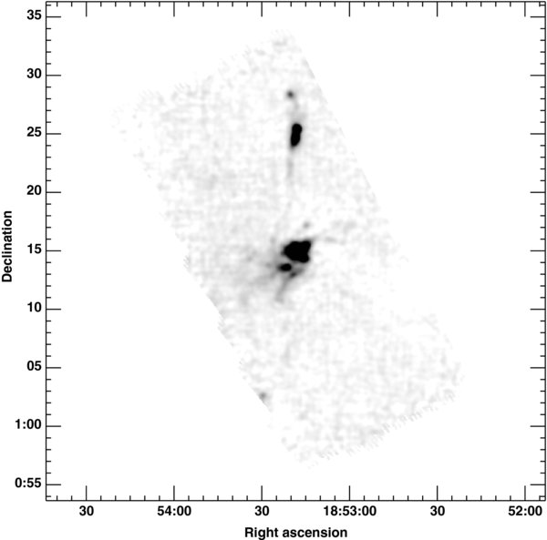
Figure 1. Observation of the star-forming region G34.3+0.2 obtained with SCUBA using the 850 μm detector array at the JCMT in 2000. These observations were carried out as an initial test for the mapping observations described in this paper. The imaged region is 30' × 15' in extent and includes the "cometary" core of G34.3+0.2, which is embedded within the bright emission structure at the image center. Emission extends directly to the north, and an additional compact feature lies about 10' to the south. The intensity gray-scale is −0.05 to 1.5 Jy beam−1. The coordinate frame epoch is RJ2000.
Download figure:
Standard image High-resolution imageIn the normal use of SCUBA, 450 μm observations would have been obtained in parallel with the 850 μm data; however, because the project was classed as a medium-weather program, the 450 μm data would have been unproductive and these bolometers were turned off during the present observations. In addition, the initial series of observations of the full program in 2003 demonstrated that the zenith atmospheric transmission limit ("weather band") initially granted resulted in insufficient signal/noise ratios, and we were able to obtain observations in 2004 under considerably better conditions. During the latter observing period half of the region observed in 2003 was observed a second time to offset the effect of the relatively poor conditions encountered during the early observations.
2.1.1. Observations at 850 μm
The region to be observed was divided into 16 segments each 30 × 15 arcmin in extent. The center positions of these are given in Table 1 together with an observing log for the observations and the mean zenith optical depth at 225 GHz (τ225), normally available from the Caltech Submillimeter Observatory, located nearby on Mauna Kea. The optical depth at 850 μm (353 GHz) is approximately four times that at 225 GHz, and the relationship between these values is well determined (Archibald et al. 2002). To obtain the zenith opacity at 850 μm we used either the nightly polynomial fits to τ225, available via the JCMT Web site, or extrapolations between values measured by skydips performed at the JCMT during the observations.
Table 1. Observing Log: SCUBA 850 μm Observations
| Field | Observation Date | ℓa | ba | τ(225)b | rms noisec |
|---|---|---|---|---|---|
| 01 | 2004 Apr 05 | 42.46241 | −0.09627 | 0.085 | 0.07 |
| 02 | 2004 Apr 05 | 42.49036 | −0.34470 | 0.085 | 0.07 |
| 03 | 2004 Apr 05 | 42.95928 | −0.04037 | 0.085 | 0.04 |
| 2004 Apr 04 | 0.090 | ||||
| 04 | 2004 Apr 04 | 42.98723 | −0.28880 | 0.080 | 0.07 |
| 05 | 2004 Apr 04 | 43.45614 | +0.01552 | 0.075 | 0.06 |
| 06 | 2004 Apr 01 | 43.48409 | −0.23291 | 0.065 | 0.05 |
| 07 | 2004 Mar 31 | 43.95301 | +0.07142 | 0.050 | 0.06 |
| 08 | 2004 Mar 30 | 43.98096 | −0.17701 | 0.055 | 0.05 |
| 09 | 2003 Aug 01 | 44.44987 | +0.12732 | 0.147 | 0.07 |
| 2003 Jul 29 | 0.150 | ||||
| 10 | 2003 Aug 01 | 44.47782 | −0.12111 | 0.135 | 0.08 |
| 2003 Jul 29 | 0.170 | ||||
| 11 | 2003 Aug 01 | 44.94674 | +0.18322 | 0.149 | 0.07 |
| 2003 Jul 29 | 0.150 | ||||
| 12 | 2003 Aug 01 | 44.97469 | −0.06521 | 0.146 | 0.07 |
| 2003 Jul 29 | 0.170 | ||||
| 13 | 2003 Aug 01 | 45.44360 | +0.23911 | 0.146 | 0.10 |
| 14 | 2003 Aug 01 | 45.47155 | −0.00932 | 0.146 | 0.10 |
| 15 | 2003 Jul 31 | 45.94047 | +0.29501 | 0.146 | 0.15 |
| 16 | 2003 Aug 01 | 45.96842 | −0.04658 | 0.146 | 0.12 |
Notes. aGalactic coordinates of the central position of each field. bZenith optical depth at 225 GHz (1300 μm); to obtain the equivalent value for the observing wavelength of 850 μm, multiply these numbers by a factor of about 4. crms noise value (Jy beam−1 pixel−1) in the final map, as determined from regions free of source emission. For regions where there was more than one observation this is the value for the combined data.
Download table as: ASCIITypeset image
Each segment was observed at 850 μm in the standard scan-mapping mode used with SCUBA, in which the subreflector was nutated at 8 Hz while the telescope was scanned across the source (Jenness et al. 2000). Equatorial coordinates were used for the observing. A total of six chop angle/direction combinations provide a complete sampling of the image plane; in this particular case two orthogonal chop directions (0° and 90°) with each of three chop distances (30'', 44'', and 68'') were used. For these observations the scanning speed was increased beyond that normally used for full sampling by a factor of 2 to 48''s−1; since only 850 μm data were being taken, this was sufficient for the present purpose. Each scan across the segment being mapped was sufficiently long to include the total extent of the segment in the scanning direction, and since the orthogonal scan directions were determined with respect to the bolometer array rather than the target region, the scan length was determined in real time. The observing process was quite efficient, each segment requiring slightly less than 1 hr for the observing. Together with calibration and other overheads, about 36 hr in total were used for this program.
For calibration purposes, one or two smaller maps (about 3' in extent) of standard sources were taken in the same manner during each observing night. Uranus and Neptune were used as the primary calibrators, although the galactic objects CRL 2688 and 16293 − 2422 also were used on occasion, depending on availability. The planetary data were used also to obtain the effective beamwidth at half-power; in the 2003 observing sessions the observations of Uranus gave a mean value of 15 2, while Neptune was used to derive a mean value of 146 during the 2004 observing sessions. The slight difference in the two values was likely a result of differing dish surface adjustments, ambient temperatures, and prevailing sky conditions at the two epochs.
2.1.2. Data Processing and Calibration
The initial stages of the reduction of the 850 μm data were carried out using the standard software available at the time (Holland et al. 1999) to flat-field the data, correct for extinction, and remove sky noise. The noise responses of the individual bolometers were first inspected to identify, and eliminate, pixels with high noise prior to the initial data processing. This initial processed data set was then used to identify other cases of high noise values before re-processing the data with poorer data omitted. The standard SCUBA reduction sequence (SURF; Jenness & Lightfoot 1998) was used via the online reduction facility ORAC-DR (Jenness & Economou 1999) to produce the final processed data set with extinction correction, baseline subtraction, and sky corrections included.
These data were then processed to construct images of the sky with a pixel size of 4 arcsec. We used both the standard facility rebinning/dual-beam removal process and a direct matrix inversion method (Johnstone et al. 2000) to produce versions of the final image with a pixel size of 4''. Since the largest chop throw employed in the observations was 68'', any structure in the reconstructed images on scales larger than this value is suspect; nevertheless, features with high aspect ratios should be correctly reproduced in any case. For the present rather inhomogeneous data set (as regards data quality), the standard data reduction tools introduced undulations in the images which are very unlikely to be real. The matrix inversion technique produced images of rather better quality in this regard and form the basis of the analysis in the present paper.
The JCMT SCUBA data were calibrated with a single value of the instrumental gain (203 Jy V−1 beam−1) derived from the ensemble of calibrator observations (see Section 2.1.1). The latter were observed in the same way as for the program fields, although covering a much smaller area. The observations of Neptune and Uranus were given the stronger weighting in this determination. Values from individual observing sessions varied by as much as 15% about the mean, and the overall calibration accuracy of the final image is set by the latter uncertainty.
2.1.3. Image Quality at 850 μm
The products of the matrix inversion are the reconstructed image of the sky, together with maps of the noise and the number of measurements at each point. For the present observations these data are shown in Figure 2 for an overview of the results. On the scale presented in this figure (note the beam size in the lower left corner of the left panel), there is little discernible detail, although the brightest submillimeter wavelength sources are clearly visible. The middle and left panels, respectively, show the rms noise level and number of measurements at each data point in the reconstructed image. Observational data for each field contain information somewhat (about 1') beyond the formal edges of the field. The resultant overlap regions between neighboring fields therefore have correspondingly more observations per point, and hence lower noise values, resulting in the pronounced orthogonal pattern evident in the "noise" and "number" images.
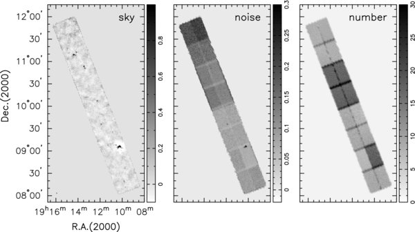
Figure 2. Region observed with SCUBA at 850 μm, following matrix inversion image reconstruction. The three panels are, from left to right, (a) the reconstructed image (labeled "sky") with an intensity scale in Jy beam−1, (b) noise values ("noise") with an intensity scale in Jy beam−1 pixel−1, and (c) the number of observations per data point ("number"). The vertical bar to the right of each panel indicates the gray-scale intensity range for that image. "Ghost" images of the brightest sources appear in the noise map, resulting from Poisson noise. The beam size (about 15'') is indicated (by the small dot) at the lower left corner of the "sky" panel, and the image is constructed using a pixel size of 4''.
Download figure:
Standard image High-resolution imageThere is substantial variation overall in the rms noise across the 850 μm image. The maximum noise values occur in the northern part of the field, where there are fewer observational samples per data point and the sky transmission was relatively poor during the time in which these data were taken (see Table 1). In the least noisy region (field 3) the rms noise level is below 0.1 Jy beam−1 pixel−1, as compared to almost 0.3 Jy beam−1 pixel−1 in the worst case. In the former region, two observations were made, both under good sky conditions, whereas only a single observation under relative poor conditions was obtained for the latter. The maximum number of observations per point in the reconstructed image, 51, occurs in this region, together with fields 9–12; however, in the worst cases (fields 13–16, in the northern part of the region), the sky transmission was relatively poor, and the number of observations limited, for all the observations.
2.2. Image Refinement and Observational Results at 850 μm
The sky image obtained at 850 μm (shown in the left panel of Figure 2) clearly shows residual low-level undulations on scales larger than the maximum chop throw. These are most likely due to bolometer gain drifts and short-term opacity variations. As an aid to subsequent analysis, we filtered out these effects by subtracting a smoothed version of the image, including only the low-level emission, from the original. We first clipped the image in Figure 2 at ±0.5 Jy beam−1 and convolved the resulting image with a two-dimensional Gaussian of width 31 pixels (i.e., 124''). This smoothed image was subtracted from the original data. Further, to facilitate comparison with the 1200 μm data, the smoothed image was convolved to an effective beam of 22''. The calibration of the final image was checked against the JCMT Legacy Catalogue (Di Francesco et al. 2008) and the source peaks were found to be in agreement to within 20%.
Figure 3 displays the final image, revealing a significant improvement in image quality; in particular, the base level in these data is considerably flatter on a scale of a few arcminutes than that for the initial image derived from the matrix inversion procedure. Also, the variation in the noise level across the image is now rather obvious, and a substantial number of submillimeter wavelength sources are clearly visible even at this reduced angular scale.

Figure 3. 850 μm image shown in Figure 2 following additional processing to remove large-scale features and smooth to an effective resolution of 22'' (see Section 2.2). The resulting flattened image is shown on an intensity scale of 0.0–1.6 Jy beam−1. Lower noise levels in the regions where map segments overlap are evident. The beam size is shown by the small dot at lower left. Galactic longitude is indicated on the two diagonal lines, drawn at Galactic latitudes of +0.5 and −05, at upper right and lower left, respectively. The square boxes show the locations and extents of three regions which are expanded to show typical image detail, respectively, from top to bottom, in Figures 4, 5 and 6.
Download figure:
Standard image High-resolution imageTo summarize these basic data, the measured rms noise for each segment ("Field") of this final map is included in Table 1. These values were determined in each case over a square area 50 pixels on a side from a region judged largely free of localized emission from the individual dust clumps. The noise values obtained are significantly improved over those for the original reconstructed map shown in Figure 2, mostly due to the smoothing to larger effective beam size.
On the scale of the entire image shown in Figure 3, it is not possible to obtain a good assessment of the image quality in regard to the detection of emission from dust in this part of the Galactic plane. For this purpose, we select three relatively small regions, indicated by the squares overlaid on Figure 3, and show these sections of the image on a common intensity scale (−0.6 to 0.3 Jy beam−1), chosen to emphasize low-level structure in the data, in Figures 4, 5 and 6. Each region is about 17' square.
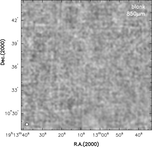
Figure 4. Region of the 850 μm image (corresponding to the upper square in Figure 3) containing no detected sources of emission. The intensity scale used, −0.6 to 0.3 Jy beam−1, was chosen to illustrate the nature of the background noise properties, as well as accentuate the lower-level image properties, to good effect. The effective beam size of the data is 22'' (shown by the circle, at lower left). The faint striations seen in this image are due to the scanning technique used to obtain the data and the slightly different noise responses of individual bolometers.
Download figure:
Standard image High-resolution image
Figure 5. Region from the 850 μm image showing typical "field" sources. Seven objects meeting the detection criteria of the clump-finding procedure are identified by crosses (see Section 3), although visual inspection and comparison with Figure 4 suggests that there is additional structure below the formal intensity cutoff level (about 0.2 Jy beam−1). The plotted contours are for 0.5, 2, and 4 Jy beam−1.
Download figure:
Standard image High-resolution image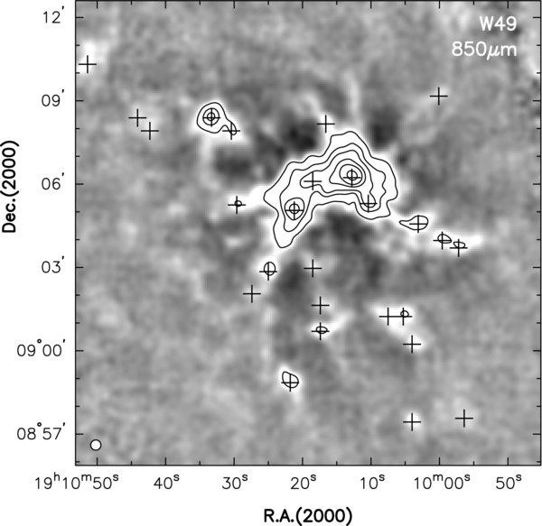
Figure 6. W49 region at 850 μm, shown on the same angular scale and intensity range as the previous two images. Contour levels are shown for 0.5, 2, 4, 10, 20, and 50 Jy beam−1. The bright central structure of W49 is surrounded by a depression in the base level resulting from the chopping technique used to obtain the image. The region is surrounded by complex filamentary and clumped structures, which are apparent throughout the image field. In the area covered by this image a total of 26 dust clumps are identified by the clump-finding routine, at the positions indicated by the crosses, and as described in Section 3.
Download figure:
Standard image High-resolution imageFigure 4, labeled "blank," shows a section of the image in which there are no obvious emission sources, and which therefore illustrates the nature of the background noise in the data at 850 μm. Faint linear structures are due to the residual noise characteristics of individual bolometers resulting from the orthogonal pattern in which the SCUBA array was scanned across the region.
The second field is shown in Figure 5; seven compact structures in this part of the image are subsequently identified by an automated clump-finding algorithm, as indicated by the crosses, and as described in Section 3. The number of dust clumps found in this map segment is typical of the average for the entire surveyed region. There are additional structures visible in this image which are likely to be weak 850 μm emission from dust, evident from comparison of the characteristics of this image with the "blank" field in Figure 4.
The third map section, in Figure 6, contains the star-forming region W49, the source of the most intense emission in the entire surveyed area. This image reveals in detail extensive ridges and clumps of dust emission surrounding the core of W49. The latter is situated within a depression in the base level caused by the chop-scanning observing method used. The flattening process described above cannot significantly remove this instrumental artifact. In this image, in particular, there is substantial evidence of clumped and filamentary dust structures below the formal clump sensitivity limit, especially to the southeast of W49. Again, comparison of this last image with Figure 4 indicates that these weak features represent real emission from dust rather than instrumental artifacts.
2.3. Observations at 1200 μm
In a companion study to the 850 μm imaging, 1200 μm observations were obtained using SIMBA (Sest IMaging Bolometer Array), a 37-element bolometer array mounted on the SEST 15 m antenna, and were carried out during 2003 August just prior to the closure of this facility. At this wavelength the beamwidth to half-power was 22''. These observations used a direct-detection method (Fastscanning) which employed rapid scanning of the target region at 160'' s−1. The data were sampled at 128 MHz and the atmospheric contribution removed in software (Reichertz et al. 2001; Weferling et al. 2002). The Fastscanning mode does not restrict the scanning speed, and allows large areas of sky to be observed in relatively short timeframes. The irregular border of the mapped region, contrasted with that of the 850 μm image, is a by-product of the automated Fastscanning technique. The flux conversion factor for these observations was 65 mJy count−1 beam−1.
3. ANALYSIS OF THE CONTINUUM IMAGE VIA CLUMP-FINDING
The final 850 μm image was used to locate and obtain the basic parameters of the compact objects within the region. For this purpose we used a two-dimensional version of the clump-finding algorithm clfind (Williams et al. 1994). In this implementation, the shapes of individual clumps are not pre-defined and each map cell in which the signal is above a given threshold is assigned to a particular "clump" or coherent structure. Johnstone et al. (2001) present an extensive discussion of this particular approach, and their article should be consulted for detailed information on the methodology.
As noted in Section 2.1.3, the 850 μm image has significant differences in the noise level between the individual sections observed. However, the noise level within any given map section does not vary significantly, except close to the perimeter, where there are fewer data points per beam area. The noise is also enhanced in pixels which record strong continuum emission sources. In order to define a set of clumps according to a coherent minimum standard, we first used the clfind program to search for signal clumps with peak emission five times the lowest overall noise level in the map. From these we eliminated clumps with peaks less than five times the local (that is, within each section) noise level. Next, to eliminate spuriously identified clumps, we removed those with areas smaller than that of the beam (i.e., incorporating less than 25 pixels) and objects very close to the map edge, where the local noise level is especially elevated. Finally, we removed remaining apparent noise spikes through visual inspection.
A total of 132 clumps survived the detection criteria. The data for these are presented in Table 2, where each clump is identified by a running number and its galactic coordinates. The list is ordered in decreasing galactic longitude. The spatial distribution of these objects is displayed in Figure 7, where we indicate also the relative sizes of the clumps. This shows that there are three major groupings of submillimeter wavelength continuum clumps, around the G45.1 and G45.5 regions in the north, and associated with the W49 star-forming region in the south, where 26 clumps were identified within the field of view shown in Figure 6.
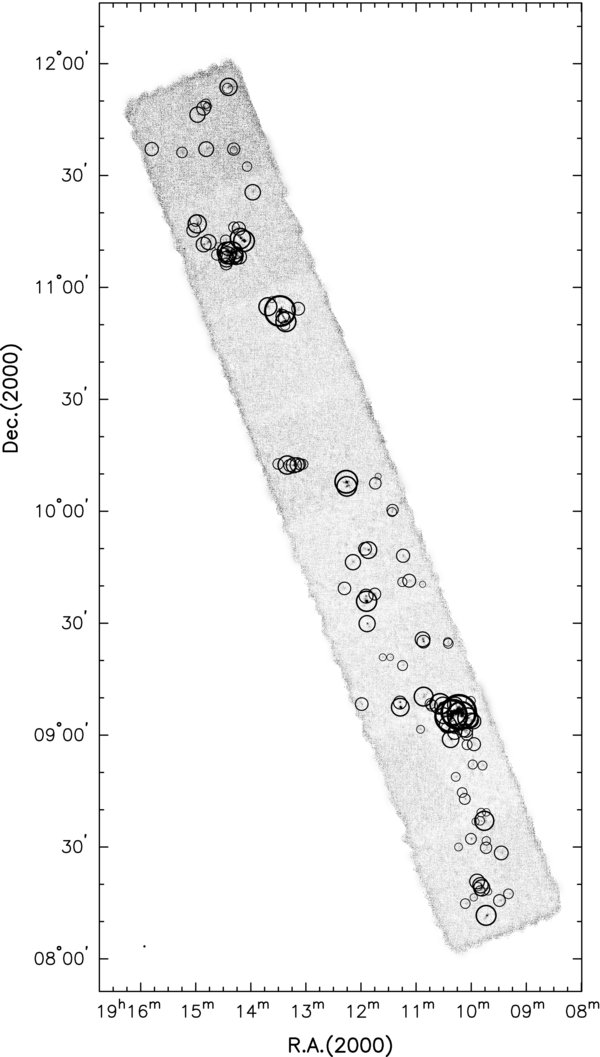
Figure 7. Distribution of clumps identified by the clfind routine, superposed on the 850 μm image (see Figure 3). Each clump is identified by a circle, the size of which is proportional to the effective radius Reff (see Table 2), and enlarged for visibility; the actual sizes of the clumps are much smaller, and can be seen in some cases within the circles.
Download figure:
Standard image High-resolution imageTable 2. Clumps Identified in the 850 μm Image
| Clump Number | Namea | R.A.b (J2000.0) | Decl. b (J2000.0) | P850c (Jy/bm) | S850c (Jy) | Reffc ('') | P1200d (Jy/bm) | S1200d (Jy) |
|---|---|---|---|---|---|---|---|---|
| 1 | G46.117+0.395 | 19:14:23.9 | 11:53:48 | 1.08 | 3.32 | 34.8 | 0.27 | 0.54 |
| 2 | G46.115+0.388 | 19:14:25.2 | 11:53:28 | 0.88 | 1.01 | 20.8 | 0.24 | 0.22 |
| 3 | G46.098+0.269 | 19:14:49.2 | 11:49:15 | 0.70 | 0.81 | 19.6 | 0.25 | 0.15 |
| 4 | G46.085+0.253 | 19:14:51.1 | 11:48:07 | 1.21 | 2.17 | 27.9 | 0.38 | 0.57 |
| 5 | G46.083+0.271 | 19:14:47.0 | 11:48:32 | 0.51 | 0.45 | 16.4 | 0.09 | 0.05 |
| 6 | G46.071+0.215 | 19:14:57.9 | 11:46:19 | 0.95 | 1.98 | 30.9 | 0.13 | 0.25 |
| 7 | G46.031 − 0.036 | 19:15:47.6 | 11:37:10 | 0.62 | 1.25 | 26.9 | 0.16 | 0.24 |
| 8 | G45.955+0.076 | 19:15:14.6 | 11:36:15 | 0.44 | 0.83 | 21.6 | 0.12 | 0.16 |
| 9 | G45.918+0.178 | 19:14:48.3 | 11:37:08 | 0.62 | 1.76 | 29.8 | 0.11 | 0.22 |
| 10 | G45.861+0.287 | 19:14:18.3 | 11:37:09 | 0.51 | 1.04 | 24.8 | 0.05 | 0.08 |
| 11 | G45.856+0.284 | 19:14:18.3 | 11:36:49 | 0.55 | 0.39 | 15.0 | 0.05 | 0.03 |
| 12 | G45.764+0.302 | 19:14:03.9 | 11:32:26 | 0.51 | 0.59 | 19.3 | 0.10 | 0.05 |
| 13 | G45.657 − 0.013 | 19:15:00.1 | 11:17:57 | 0.53 | 0.94 | 23.4 | 0.12 | 0.18 |
| 14 | G45.651+0.272 | 19:13:57.6 | 11:25:34 | 0.51 | 1.46 | 31.2 | 0.15 | 0.37 |
| 15 | G45.640 − 0.013 | 19:14:58.2 | 11:17:05 | 1.10 | 3.25 | 36.7 | 0.29 | 0.93 |
| 16 | G45.622 − 0.040 | 19:15:02.0 | 11:15:21 | 0.57 | 1.05 | 27.3 | 0.16 | 0.30 |
| 17 | G45.551+0.125 | 19:14:18.2 | 11:16:10 | 0.40 | 0.61 | 21.6 | 0.11 | 0.14 |
| 18 | G45.545 − 0.030 | 19:14:51.1 | 11:11:33 | 0.95 | 2.00 | 30.0 | 0.17 | 0.37 |
| 19 | G45.544 − 0.007 | 19:14:45.9 | 11:12:09 | 1.03 | 2.24 | 30.6 | 0.30 | 0.48 |
| 20 | G45.536+0.141 | 19:14:12.8 | 11:15:50 | 0.70 | 1.20 | 26.7 | 0.11 | 0.18 |
| 21 | G45.516+0.066 | 19:14:26.9 | 11:12:42 | 0.40 | 0.63 | 21.6 | 0.16 | 0.15 |
| 22 | G45.506+0.025 | 19:14:34.7 | 11:10:58 | 0.33 | 0.27 | 15.3 | 0.13 | 0.07 |
| 23 | G45.493+0.127 | 19:14:11.1 | 11:13:10 | 2.46 | 6.85 | 41.0 | 0.68 | 2.53 |
| 24 | G45.478+0.056 | 19:14:24.7 | 11:10:22 | 0.59 | 1.60 | 27.0 | 0.16 | 0.35 |
| 25 | G45.477+0.002 | 19:14:36.4 | 11:08:50 | 0.40 | 0.69 | 22.0 | 0.18 | 0.15 |
| 26 | G45.475+0.135 | 19:14:07.3 | 11:12:26 | 4.33 | 12.21 | 41.9 | 1.33 | 5.34 |
| 27 | G45.466+0.046 | 19:14:25.5 | 11:09:30 | 6.91 | 16.98 | 39.6 | 2.25 | 5.33 |
| 28 | G45.463+0.029 | 19:14:28.8 | 11:08:50 | 1.39 | 1.92 | 26.0 | 0.32 | 0.32 |
| 29 | G45.455+0.062 | 19:14:20.9 | 11:09:18 | 5.41 | 17.32 | 45.4 | 2.49 | 7.96 |
| 30 | G45.455+0.040 | 19:14:25.5 | 11:08:42 | 1.12 | 4.64 | 34.9 | 0.38 | 0.93 |
| 31 | G45.446+0.082 | 19:14:15.5 | 11:09:22 | 0.66 | 1.31 | 24.1 | 0.17 | 0.24 |
| 32 | G45.440+0.029 | 19:14:26.3 | 11:07:38 | 0.53 | 1.80 | 31.7 | 0.13 | 0.32 |
| 33 | G45.434+0.078 | 19:14:14.9 | 11:08:38 | 0.68 | 1.79 | 26.6 | 0.21 | 0.26 |
| 34 | G45.426+0.069 | 19:14:16.0 | 11:07:58 | 0.51 | 1.10 | 27.6 | 0.16 | 0.31 |
| 35 | G45.423+0.084 | 19:14:12.4 | 11:08:14 | 1.10 | 2.11 | 29.0 | 0.19 | 0.31 |
| 36 | G45.422+0.018 | 19:14:26.6 | 11:06:22 | 0.37 | 0.76 | 24.0 | 0.11 | 0.18 |
| 37 | G45.187+0.125 | 19:13:36.8 | 10:56:51 | 0.29 | 0.19 | 13.2 | 0.09 | 0.06 |
| 38 | G45.166+0.093 | 19:13:41.4 | 10:54:51 | 0.55 | 1.86 | 36.3 | 0.16 | 0.51 |
| 39 | G45.123+0.133 | 19:13:27.8 | 10:53:39 | 10.01 | 32.20 | 60.4 | 5.39 | 16.08 |
| 40 | G45.098+0.132 | 19:13:25.1 | 10:52:19 | 0.88 | 1.88 | 26.9 | 0.22 | 0.34 |
| 41 | G45.094+0.209 | 19:13:08.0 | 10:54:15 | 0.33 | 0.85 | 26.0 | 0.10 | 0.18 |
| 42 | G45.086+0.134 | 19:13:23.5 | 10:51:43 | 0.77 | 1.47 | 24.1 | 0.24 | 0.47 |
| 43 | G45.071+0.133 | 19:13:21.9 | 10:50:55 | 10.16 | 16.30 | 40.4 | 3.03 | 6.28 |
| 44 | G45.057+0.123 | 19:13:22.4 | 10:49:51 | 0.35 | 0.47 | 19.2 | 0.10 | 0.05 |
| 45 | G44.523 − 0.192 | 19:13:30.1 | 10:12:43 | 0.33 | 0.55 | 21.5 | 0.10 | 0.06 |
| 46 | G44.499 − 0.158 | 19:13:20.1 | 10:12:24 | 0.59 | 2.39 | 37.0 | 0.13 | 0.36 |
| 47 | G44.492 − 0.149 | 19:13:17.4 | 10:12:16 | 0.55 | 1.06 | 24.3 | 0.16 | 0.17 |
| 48 | G44.484 − 0.132 | 19:13:12.8 | 10:12:20 | 0.86 | 1.96 | 30.7 | 0.17 | 0.25 |
| 49 | G44.481 − 0.118 | 19:13:09.3 | 10:12:32 | 0.40 | 1.03 | 28.7 | 0.08 | 0.12 |
| 50 | G44.475 − 0.105 | 19:13:06.0 | 10:12:36 | 0.42 | 0.80 | 23.0 | 0.15 | 0.13 |
| 51 | G44.470 − 0.094 | 19:13:03.0 | 10:12:36 | 0.44 | 0.62 | 20.8 | 0.16 | 0.17 |
| 52 | G44.311+0.042 | 19:12:15.6 | 10:07:56 | 3.59 | 9.02 | 45.5 | 0.75 | 2.40 |
| 53 | G44.292+0.034 | 19:12:15.1 | 10:06:44 | 1.21 | 3.63 | 39.5 | 0.32 | 0.93 |
| 54 | G44.266+0.179 | 19:11:40.9 | 10:09:24 | 0.33 | 0.20 | 12.8 | 0.04 | 0.01 |
| 55 | G44.245+0.153 | 19:11:44.2 | 10:07:32 | 0.48 | 0.73 | 23.7 | 0.19 | 0.22 |
| 56 | G44.104+0.167 | 19:11:25.3 | 10:00:24 | 0.40 | 0.69 | 23.1 | 0.13 | 0.15 |
| 57 | G44.096+0.160 | 19:11:25.8 | 09:59:48 | 0.55 | 0.59 | 18.6 | 0.13 | 0.13 |
| 58 | G44.006 − 0.023 | 19:11:55.3 | 09:49:56 | 0.44 | 0.91 | 26.0 | 0.09 | 0.12 |
| 59 | G43.995 − 0.011 | 19:11:51.5 | 09:49:40 | 1.54 | 2.77 | 33.7 | 0.30 | 0.54 |
| 60 | G43.979 − 0.098 | 19:12:08.3 | 09:46:24 | 0.62 | 1.40 | 30.8 | 0.17 | 0.28 |
| 61 | G43.900+0.113 | 19:11:13.9 | 09:48:03 | 0.48 | 0.93 | 26.6 | 0.12 | 0.16 |
| 62 | G43.892 − 0.187 | 19:12:17.8 | 09:39:20 | 0.31 | 0.68 | 25.4 | 0.11 | 0.11 |
| 63 | G43.817 − 0.117 | 19:11:54.3 | 09:37:16 | 0.64 | 1.44 | 28.3 | 0.14 | 0.28 |
| 64 | G43.807 − 0.077 | 19:11:44.5 | 09:37:52 | 0.48 | 0.85 | 24.2 | 0.14 | 0.16 |
| 65 | G43.799+0.056 | 19:11:14.8 | 09:41:07 | 0.33 | 0.40 | 18.8 | 0.11 | 0.07 |
| 66 | G43.795 − 0.126 | 19:11:53.7 | 09:35:52 | 9.75 | 16.04 | 40.7 | 2.53 | 5.23 |
| 67 | G43.789+0.086 | 19:11:07.2 | 09:41:23 | 0.33 | 0.78 | 26.2 | 0.11 | 0.20 |
| 68 | G43.747+0.132 | 19:10:52.6 | 09:40:27 | 0.24 | 0.16 | 12.8 | 0.05 | 0.01 |
| 69 | G43.706 − 0.169 | 19:11:52.9 | 09:29:56 | 1.08 | 1.89 | 32.6 | 0.24 | 0.48 |
| 70 | G43.540 − 0.178 | 19:11:36.2 | 09:20:52 | 0.26 | 0.23 | 14.4 | 0.14 | 0.06 |
| 71 | G43.530+0.018 | 19:10:52.7 | 09:25:43 | 0.95 | 2.06 | 30.0 | 0.28 | 0.65 |
| 72 | G43.524 − 0.147 | 19:11:27.8 | 09:20:52 | 0.26 | 0.20 | 13.7 | 0.08 | 0.03 |
| 73 | G43.518+0.016 | 19:10:51.8 | 09:25:03 | 1.08 | 1.76 | 25.7 | 0.27 | 0.50 |
| 74 | G43.468+0.112 | 19:10:25.4 | 09:25:03 | 0.33 | 0.39 | 17.5 | 0.10 | 0.07 |
| 75 | G43.466 − 0.115 | 19:11:14.3 | 09:18:40 | 0.31 | 0.45 | 20.3 | 0.18 | 0.16 |
| 76 | G43.460+0.111 | 19:10:24.8 | 09:24:35 | 0.33 | 0.49 | 19.7 | 0.14 | 0.14 |
| 77 | G43.398 − 0.357 | 19:11:58.9 | 09:08:20 | 0.44 | 0.89 | 25.7 | 0.19 | 0.16 |
| 78 | G43.326 − 0.202 | 19:11:17.3 | 09:08:48 | 1.08 | 1.55 | 26.1 | 0.32 | 0.35 |
| 79 | G43.307 − 0.211 | 19:11:17.0 | 09:07:32 | 4.77 | 7.70 | 35.8 | 1.52 | 2.62 |
| 80 | G43.300 − 0.096 | 19:10:51.6 | 09:10:19 | 0.48 | 2.06 | 38.0 | 0.11 | 0.38 |
| 81 | G43.258 − 0.085 | 19:10:44.4 | 09:08:23 | 0.29 | 0.47 | 21.3 | 0.05 | 0.06 |
| 82 | G43.247 − 0.082 | 19:10:42.5 | 09:07:55 | 0.31 | 0.59 | 22.4 | 0.09 | 0.10 |
| 83 | G43.237 − 0.046 | 19:10:33.6 | 09:08:23 | 5.57 | 11.34 | 41.2 | 2.19 | 5.16 |
| 84 | G43.224 − 0.038 | 19:10:30.6 | 09:07:55 | 0.70 | 2.15 | 33.4 | 0.52 | 1.68 |
| 85 | G43.202+0.014 | 19:10:16.8 | 09:08:11 | 0.53 | 1.50 | 31.1 | 0.56 | 1.04 |
| 86 | G43.185+0.082 | 19:10:00.3 | 09:09:10 | 0.26 | 0.37 | 18.9 | 0.14 | 0.15 |
| 87 | G43.183 − 0.056 | 19:10:29.8 | 09:05:15 | 0.62 | 1.90 | 31.7 | 0.08 | 0.05 |
| 88 | G43.177 − 0.176 | 19:10:54.9 | 09:01:36 | 0.35 | 0.34 | 16.3 | 0.06 | 0.03 |
| 89 | G43.175 − 0.009 | 19:10:18.7 | 09:06:07 | 6.62 | 35.75 | 50.9 | 4.00 | 13.60 |
| 90 | G43.166+0.013 | 19:10:13.1 | 09:06:15 | 77.77 | 236.14 | 68.8 | 31.14 | 102.94 |
| 91 | G43.164 − 0.027 | 19:10:21.4 | 09:05:03 | 16.17 | 50.03 | 64.0 | 7.44 | 17.64 |
| 92 | G43.148+0.015 | 19:10:10.6 | 09:05:19 | 6.56 | 29.03 | 54.8 | 3.19 | 15.07 |
| 93 | G43.139 − 0.058 | 19:10:25.2 | 09:02:51 | 0.79 | 2.16 | 33.9 | 0.31 | 0.93 |
| 94 | G43.132 − 0.073 | 19:10:27.7 | 09:02:03 | 0.24 | 0.31 | 17.5 | 0.12 | 0.13 |
| 95 | G43.129 − 0.033 | 19:10:18.7 | 09:02:59 | 0.31 | 0.22 | 13.9 | 0.11 | 0.06 |
| 96 | G43.123+0.036 | 19:10:03.3 | 09:04:35 | 0.97 | 3.60 | 40.6 | 0.44 | 1.85 |
| 97 | G43.108+0.044 | 19:09:59.8 | 09:03:58 | 0.70 | 1.66 | 29.5 | 0.27 | 0.72 |
| 98 | G43.107 − 0.040 | 19:10:17.7 | 09:01:39 | 0.26 | 0.38 | 19.2 | 0.06 | 0.06 |
| 99 | G43.099+0.050 | 19:09:57.4 | 09:03:42 | 0.62 | 1.76 | 30.5 | 0.23 | 0.37 |
| 100 | G43.093 − 0.047 | 19:10:17.7 | 09:00:43 | 0.68 | 1.47 | 28.3 | 0.17 | 0.32 |
| 101 | G43.082 − 0.006 | 19:10:07.7 | 09:01:15 | 0.53 | 1.17 | 25.8 | 0.13 | 0.30 |
| 102 | G43.078+0.002 | 19:10:05.5 | 09:01:15 | 0.64 | 1.41 | 27.6 | 0.22 | 0.45 |
| 103 | G43.074 − 0.077 | 19:10:22.0 | 08:58:51 | 1.08 | 2.42 | 33.2 | 0.27 | 0.75 |
| 104 | G43.061 − 0.001 | 19:10:04.2 | 09:00:15 | 0.53 | 0.84 | 23.8 | 0.17 | 0.37 |
| 105 | G43.019 − 0.023 | 19:10:04.2 | 08:57:27 | 0.48 | 0.63 | 20.4 | 0.17 | 0.17 |
| 106 | G43.007+0.006 | 19:09:56.6 | 08:57:35 | 0.22 | 0.67 | 26.3 | 0.09 | 0.08 |
| 107 | G42.930 − 0.041 | 19:09:58.0 | 08:52:11 | 0.31 | 0.38 | 18.5 | 0.13 | 0.07 |
| 108 | G42.916 − 0.133 | 19:10:16.4 | 08:48:51 | 0.31 | 0.37 | 18.2 | 0.05 | 0.04 |
| 109 | G42.906 − 0.004 | 19:09:47.5 | 08:51:54 | 0.26 | 0.36 | 18.5 | 0.09 | 0.06 |
| 110 | G42.839 − 0.141 | 19:10:09.4 | 08:44:35 | 0.22 | 0.38 | 19.9 | 0.10 | 0.06 |
| 111 | G42.809 − 0.144 | 19:10:06.7 | 08:42:55 | 0.44 | 0.61 | 22.2 | 0.12 | 0.14 |
| 112 | G42.721 − 0.106 | 19:09:48.7 | 08:39:15 | 0.35 | 0.37 | 17.5 | 0.15 | 0.14 |
| 113 | G42.712 − 0.086 | 19:09:43.3 | 08:39:19 | 0.22 | 0.23 | 15.5 | 0.17 | 0.07 |
| 114 | G42.697 − 0.147 | 19:09:54.9 | 08:36:51 | 0.37 | 0.28 | 14.8 | 0.11 | 0.07 |
| 115 | G42.690 − 0.127 | 19:09:49.8 | 08:36:59 | 0.33 | 0.38 | 17.6 | 0.09 | 0.07 |
| 116 | G42.681 − 0.112 | 19:09:45.5 | 08:36:59 | 0.40 | 2.04 | 38.5 | 0.15 | 0.46 |
| 117 | G42.638 − 0.202 | 19:10:00.1 | 08:32:12 | 0.57 | 0.79 | 22.1 | 0.16 | 0.16 |
| 118 | G42.632 − 0.268 | 19:10:13.6 | 08:30:04 | 0.26 | 0.28 | 16.1 | 0.06 | 0.03 |
| 119 | G42.598 − 0.144 | 19:09:43.1 | 08:31:39 | 0.29 | 0.34 | 17.5 | 0.11 | 0.09 |
| 120 | G42.572 − 0.160 | 19:09:43.7 | 08:29:51 | 0.31 | 0.62 | 23.2 | 0.14 | 0.15 |
| 121 | G42.520 − 0.110 | 19:09:27.0 | 08:28:27 | 0.35 | 0.84 | 27.8 | 0.09 | 0.10 |
| 122 | G42.457 − 0.265 | 19:09:53.4 | 08:20:48 | 0.51 | 1.29 | 29.8 | 0.23 | 0.33 |
| 123 | G42.435 − 0.259 | 19:09:49.7 | 08:19:48 | 1.89 | 2.92 | 31.0 | 0.73 | 1.03 |
| 124 | G42.434 − 0.272 | 19:09:52.4 | 08:19:24 | 0.29 | 0.32 | 17.0 | 0.20 | 0.16 |
| 125 | G42.422 − 0.260 | 19:09:48.3 | 08:19:04 | 0.79 | 2.48 | 32.6 | 0.35 | 0.74 |
| 126 | G42.414 − 0.271 | 19:09:49.9 | 08:18:20 | 0.35 | 0.52 | 19.9 | 0.20 | 0.18 |
| 127 | G42.401 − 0.311 | 19:09:57.0 | 08:16:32 | 0.31 | 0.26 | 15.1 | 0.07 | 0.02 |
| 128 | G42.394 − 0.357 | 19:10:06.1 | 08:14:53 | 0.26 | 0.40 | 19.7 | 0.12 | 0.10 |
| 129 | G42.394 − 0.242 | 19:09:41.3 | 08:18:04 | 0.29 | 0.24 | 14.8 | 0.12 | 0.07 |
| 130 | G42.342 − 0.165 | 19:09:19.0 | 08:17:27 | 0.33 | 0.46 | 19.8 | 0.13 | 0.09 |
| 131 | G42.335 − 0.215 | 19:09:29.0 | 08:15:40 | 0.40 | 0.79 | 24.2 | 0.27 | 0.33 |
| 132 | G42.303 − 0.299 | 19:09:43.5 | 08:11:40 | 1.21 | 3.59 | 40.0 | 0.77 | 0.78 |
Notes. aName formed from equivalent Galactic coordinates, accurate to approximately 4''. bPosition of peak surface brightness within the clump at 850 μm (positional accuracy about 4''). cPeak flux, total flux, and effective radius of the clumps as determined by clfind (Williams et al. 1994). The absolute flux calibration is uncertain at a level of about 20%. The effective radius has not been deconvolved from the telescope beam. dPeak flux and total flux at 1200 μm determined using the 850 μm clump locations.
The major uncertainty in the flux densities obtained for the dust clumps arises from the calibration of the data. We estimate that this effect is about 20%, applicable to all the clumps identified in Table 2. In addition, the noise characteristics vary across the image, as is clearly apparent in Figure 3. Using the rms noise values in the sections of the image with the least good noise values, we obtained estimates of the errors in the clump flux densities, from which we derived estimates of the fractional errors in the total flux ranging from 4% to 8%. The varying noise level for each segment of the image results in relatively fewer weak sources being identified in the noisier regions, in particular in the northern sections of the region.
The most intense single clump (entry 90 in Table 2) is associated with the core of W49, and accounts for 37% of the total flux density from the entire region observed. Even aside from these concentrations, the distribution of clumps is far from uniform. At the south end of the map clumps appear to be confined to a relatively narrow band, while above W49 and at the higher-latitude end of the region surveyed the distribution is more extended in galactic latitude. There are no sources identified in a region somewhat larger than 05 in extent centered at declination ∼10°30' (see also Figure 4); this appears to be a real lack of objects, as the noise levels are similar to those in the rest of the region observed.
In Table 2 we include in the final two columns the integrated and peak flux densities at 1200 μm. These data were derived from the 1200 μm image using the position and footprint for each of the clumps identified at 850 μm, rather than using an independent clump search at 1200 μm. The integrated flux densities follow a linear relation for which S850 ≈ 2.3 × S1200, as shown in Figure 8. The peak flux relationship shows the same scaling. We estimate the likely uncertainty in the flux densities at 1200 μm to be similar to those at 850 μm, i.e., about 20%, with a minimum sensitivity of about 0.1 Jy beam−1.

Figure 8. Continuum flux comparison for the clump ensemble at 850 μm vs. 1200 μm. Integrated intensities (S) are plotted in the left panel while the peak fluxes ((P) within a 22'' beam) are shown in the right panel. For clarity, only the brighter clumps are included in the plots. Measurement errors (rms values are indicated by the symbol at lower right in both frames) dominate for low-flux objects while at higher flux values ∼20% systematic uncertainties in the calibration are the dominant source of error. The straight line in both plots follows a linear relation with a slope of 2.3 (see Section 3).
Download figure:
Standard image High-resolution imageMost of the clumps have integrated flux densities at 1200 μm of less than 1 Jy, and there is a substantial scatter about the mean value relation shown in the figure. The latter is at least in part due to measurement errors, but we would expect that dust temperature differences within the clump ensemble also contribute significantly to this scatter. The data are not sufficiently precise to enable us to draw firm conclusions in this regard; however, the low conversion factor of 2.3 between 850 μm and 1200 μm fluxes does require both a low dust temperature, Td < 20 K, and a low value for the dust emissivity power-law exponent, β < 2.
4. COMPARING 850 AND 1200 μm IMAGES WITH 13CO (1–0) EMISSION
The region we observed is shown projected in galactic coordinates in Figure 9. Here the SCUBA 850 μm and SIMBA/SEST 1200 μm images are placed in context with the molecular emission from the region by comparison with a velocity slice (50–70 km s−1) from the GRS 13CO (1–0) data. The latter velocity range includes the majority (two-thirds) of the dust clumps observed in the region, as determined from the GRS data and additional molecular line observations obtained in the present work.
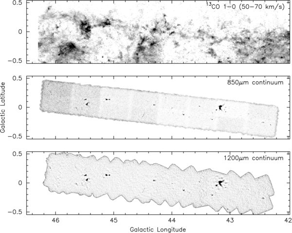
Figure 9. 850 μm (JCMT; middle panel) and 1200 μm (SEST; lower panel) data in the context of molecular line emission (upper panel), shown in Galactic coordinates. The upper panel shows the distribution of 13CO (1–0) emission integrated over an LSR velocity range of 50–70 km s−1, from the GRS data (see text); the plotted intensity range of the 13CO (1–0) emission is from 1 to 8 K km s−1 on the T*a (antenna temperature) scale. The intensity range is 0.0–1.0 Jy beam−1 for the 850 μm image and 0.0–0.5 Jy beam−1 for the 1200 SEST image. Two-thirds of the continuum clumps observed at 850 and 1200 μm in this work have LSR velocities within the range covered by the 13CO (1–0) image.
Download figure:
Standard image High-resolution imageAs noted in Section 2.3, the 1200 μm data were obtained in a direct-detection mode. In principle, this technique should ensure that no artifacts remain in this 1200 μm image, such as those which can result from the removal of the dual-beam signature in the case of the JCMT 850 μm image following removal of the dual-beam signature.
In principle, larger-scale structures should be faithfully registered in the 1200 μm data, and the base level well determined. Inspection of the 1200 μm results thus provides confirmation that there are no substantially extended bright emission structures in the 850 μm data set which, if present, would have been diminished by the chopping technique used in the latter case. Further, the relative sensitivity of the two images to small-scale structures is quite comparable; this is illustrated by comparing the detailed 850 and 1200 μm images in the following section.
However, as is obvious from Figure 9, only the highest column density regions of 13CO (1–0) emission are associated with detectable dust emission, and, conversely, the majority of the gaseous material is not associated with observable amounts of cold dust at the sensitivity levels attained in the present work. Note that W49 is not registered in the 13CO (1–0) velocity range presented in Figure 9, as its LSR velocity is about 7 km s−1.
4.1. Results for Individual Regions
Two sections of the 850 and 1200 μm images are presented in closer detail (and in equatorial coordinates) in Figures 10 and 11, where the continuum images from the present work are compared with the GRS 13CO (1–0) (using the same velocity range as for Figure 9) and 8 μm images of the same regions taken from the MSX mission (Price et al. 2001).

Figure 10. Images of millimeter and submillimeter wavelength continuum emission from the star-forming region G45.1/G45.5 from the present work at 850 μm (lower left) and 1200 μm (upper left). These are compared with 13CO (1–0) emission (from the GRS) at upper right, and the 8 μm emission observed by the MSX satellite at lower right. The beamsizes (to half-power) for the images are indicated by the circles at the lower left corner of each panel.
Download figure:
Standard image High-resolution image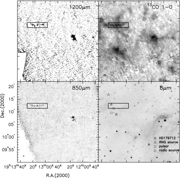
Figure 11. Vicinity of a group of dust clumps (shown within the rectangle), at a kinematic distance of 6 kpc (see text and Table 3), as observed at 1200 and 850 μm in the present paper, and in the 13CO (1–0) transition. Nearby objects in the field are indicated by the key at lower right in the MSX 8 μm image. Other details as for Figure 10.
Download figure:
Standard image High-resolution imageThe G45.1/45.5 region (see Figure 10) includes several compact H ii regions which are known to be associated with OH and H2O maser sources. At millimeter and submillimeter wavelengths the region consists of two main groups of compact objects, along with several weaker components, which appear in both images. These structures are well correlated with their appearance at mid-infrared wavelengths (e.g., at 8 μm, from the MSX mission) and with emission in the 13CO (1–0) line. Similarities in the appearance of these objects in dust, CO, and mid-IR emission are typical of images of active star-forming regions.
The latter situation contrasts with a region about a degree further south, shown in Figure 11. In this case, although there is considerable complexity in the 13CO (1–0) emission as seen by the GRS, most of the latter molecular structures are not visible in continuum emission at millimeter and submillimeter wavelengths, implying that they possess a relatively low dust column density. The exceptions are a relatively bright compact structure consisting of two main clumps to the west and an elongated feature to the east about 5' in length, both of which appear in the 850 μm and 1200 μm images, as well as in the 13CO (1–0) data. However, neither of the latter objects are visible at 8 μm or 24 μm (see Section 8.2), suggesting that they are relatively cold, dense objects which are yet to form stars, in contrast to the group of dust/gas clumps in the G45.1/G45.5 region (Figure 10).
Figure 12 focuses on the elongated feature mentioned above which is centered at G44.48 − 0.13. An expanded view of this structure shows it to consist of a series of (probably) six distinct dust clumps, terminated at the eastern extremity by an IRAS object (19110+1007) which also shows relatively weak indications of emission from dust at 850 μm. The positions determined for these dust clumps substantially predate the formal clump-finding analysis presented in Table 2 (Section 3); nevertheless, the six clumps indicated by "plus" signs in Figure 12 were independently identified in Table 2 as clumps 46–51 (from east to west). Possible dust emission associated with IRAS 19110+1007 lies below the formal detection level.

Figure 12. Expanded view of part of the 850 μm continuum structure shown (within the rectangle) in Figure 11. The locations of six submillimeter continuum clumps identified within the boundary of this image are marked by crosses. The position of IRAS 19110+1007 is indicated by a triangle.
Download figure:
Standard image High-resolution imageThe latter region was subsequently observed using the JCMT in service mode in the 13CO (3–2) transition, for which the angular resolution attained is the same as for the continuum image. These data show (Figure 13) more extensive emission from gas than that seen from dust in the 850 μm continuum, a result of the instrumental sensitivity to gas (CO) relative to that of dust emission in these observations, in addition to the more pronounced clumpiness of the latter. With the exceptions of the clumps, most of the 13CO emission is quite optically thin and contains relatively little, if any, cold dust.

Figure 13. Image of the structure shown in Figure 12, as observed in the 13CO (3–2) transition. The emission is integrated over 58–62 km s−1 (w.r.t. LSR), which covers the full velocity extent of the gas/dust clumps, and the intensity scale shown includes the range 3.5–11 K km s−1, with an uncertainty of about ±1.0 K km s−1. The locations of the six submillimeter continuum clumps identified within the boundary of this image are marked by crosses, as in Figure 12. The position of the single IRAS source within the field is indicated by the triangle; this is coincident within the errors with an MSX point source visible in Figure 11.
Download figure:
Standard image High-resolution imageUsing these data we can associate LSR velocities with five of the more compact clumps, for which the measured parameters are listed in Table 3. The clump velocities are very similar, within about 0.5 km s−1 of the mean value of 60.0 km s−1, and the velocity widths are on average within about 0.25 km s−1 of a mean value of 3.6 km s−1. These data imply that this group of clumps constitute a single elongated structure in which several potentially star-forming regions are collapsing, a unique feature within the extent of the 850/1200 μm images in this paper. The kinematic distance of this structure implied by the mean radial velocity is about 7.5 kpc (see Section 6).
Table 3. G44.484-0.133: Peak 13CO (3–2) Parameters
| Clump | Name | R.A. (J2000) | Decl. (J2000) | Amplitude K T*a | Line Width km s−1 | LSR Velocity km s−1 | Integrated K km s−1 |
|---|---|---|---|---|---|---|---|
| A | G44.515 − 0.168 | 19:13:24.1 | 10:12:58 | 3.0 | 3.5 | 60.3 | 12.4 |
| B | G44.505 − 0.165 | 19:13:22.3 | 10:12:32 | 2.4 | 4.0 | 59.7 | 9.2 |
| C | G44.488 − 0.151 | 19:13:17.2 | 10:12:00 | 2.9 | 3.8 | 59.4 | 13.1 |
| D | G44.485 − 0.134 | 19:13:13.3 | 10:12:20 | 3.1 | 3.3 | 60.3 | 10.6 |
| E | G44.473 − 0.103 | 19:13:05.1 | 10:12:32 | 2.7 | 3.3 | 60.3 | 11.6 |
Notes. These data represent the initial effort in the present program of observations to study the range of gas properties of dust clumps in star-forming regions in the Galactic plane presented in this paper. The results are nevertheless typical of the much larger field subsequently studied; rms errors for the peak amplitude and velocity are about 0.3 K T*a and 0.2 km s−1, respectively.
Download table as: ASCIITypeset image
5. BEAM-MATCHED MOLECULAR LINE OBSERVATIONS OF THE CLUMP ENSEMBLE
In 2005 August and September we undertook a more extended program of spectral line observations with the JCMT of the 13CO and 12CO (3–2) transitions of a substantial subset of the objects identified in the 850 μm continuum image. With the single-beam dual-channel receiver system available at the time, a complete map of the entire region would have required a prohibitive observing time; we therefore focused on individual targets already identified via their 850 μm continuum emission, as in the earlier observations described above.
We obtained either small maps two arcminutes in extent in the 13CO (3–2) transition, or simple integrations of five points arranged in a cross (center, and four positions offset in the cardinal directions by 30'') of the 12CO (3–2) line. The central positions observed are given in Tables 4 and 5 for the small maps and the five-point observations, respectively. We indicate the positions for these observations in Figure 14. The reference position used for these data was 5 arcmin either east or west of the central position, chosen in an endeavor to avoid probable confusion with nearby spectral line emission, as determined from visual inspection of the 850 μm continuum image of the region. For the small maps, we chose fairly bright 850 μm continuum targets, and obtained fully sampled images. A set of objects with generally weaker continuum emission were chosen for the five-point maps; in this case, our intent was simply to attempt to obtain spectra of typical weaker continuum objects, to determine kinematic distances and search for possible outflows.
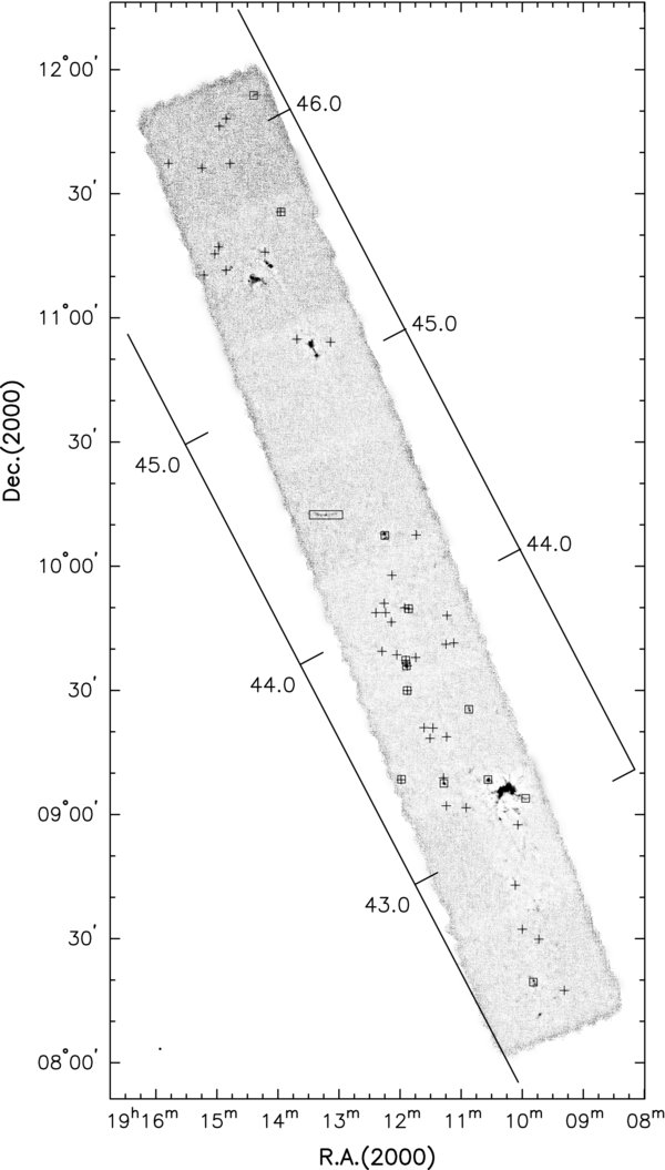
Figure 14. Distribution of spectral line observations carried out in this program, superposed on the 850 μm image of the region. Crosses and square boxes respectively indicate the locations of 12CO five-point and 13CO (3–2) map observations. The rectangle near the middle of the map indicates the location of the 13CO (3–2) map of the G44.484 − 0.133 region (see Table 3). Lines of constant galactic latitude are indicated, as in Figure 3.
Download figure:
Standard image High-resolution imageTable 4. 13CO (3–2) Mapping Observations
| Namea | R.A.b | Decl.b | Clumpc | Line Aread | Line Widthe | Line Centroidf | Distance (kpc) | Notes | |
|---|---|---|---|---|---|---|---|---|---|
| J2000 | J2000 | Number | K km s−1 | km s−1 | km s−1 | Near | Far | ||
| CO46.116+0.401 | 19:14:23.8 | 11:53:44 | 1 | 16.0 | ⋅⋅⋅ | 55.5 | 4.2 | 7.5 | |
| 2 | 14.9 | ⋅⋅⋅ | 54.3 | 4.1 | 7.7 | ||||
| CO45.650+0.275 | 19:13:56.9 | 11:25:36 | 14 | 10.0 | 2.8 | 9.6 | 0.9 | 11.0 | |
| CO44.310+0.042 | 19:12:14.9 | 10:07:26 | 52 | 52.8 | ⋅⋅⋅ | 57.6 | 4.2 | 7.9 | |
| 53 | 16.8 | 4.0 | 56.5 | 4.1 | 8.1 | ||||
| CO43.996 − 0.012 | 19:11:51.6 | 09:49:42 | 58 | 12.3 | 2.5 | 65.0 | 5.2 | 7.0 | 1 |
| 59 | 31.6 | 2.5 | 65.4 | 5.3 | 6.9 | ||||
| CO43.818 − 0.117 | 19:11:54.4 | 09:37:18 | 63 | 12.6 | 3.0 | 47.3 | 3.3 | 9.0 | 2 |
| CO43.796 − 0.126 | 19:11:53.7 | 09:35:55 | 66 | 121.9 | ⋅⋅⋅ | 44.2 | 3.0 | 9.3 | 2,3 |
| CO43.707 − 0.169 | 19:11:53.0 | 09:29:58 | 69 | 19.9 | 3.0 | 66.2 | 5.4 | 6.9 | |
| CO43.530+0.019 | 19:10:52.3 | 09:25:26 | 71 | 11.8 | ⋅⋅⋅ | 63.3 | 4.8 | 7.5 | |
| 73 | 18.7 | ⋅⋅⋅ | 61.8 | 4.6 | 7.7 | ||||
| CO43.400 − 0.355 | 19:11:58.6 | 09:08:31 | 77 | 5.9 | 1.7 | 60.2 | 4.4 | 7.9 | |
| CO43.307 − 0.210 | 19:11:17.0 | 09:07:32 | 79 | 26.8 | ⋅⋅⋅ | 58.7 | 4.2 | 8.1 | |
| CO43.238 − 0.046 | 19:10:33.7 | 09:08:25 | 83 | 83.6 | ⋅⋅⋅ | 5.7 | 0.6 | 11.8 | |
| 84 | 18.8 | 4.8 | 9.1 | 0.8 | 11.6 | ||||
| CO43.101+0.055 | 19:09:56.6 | 09:03:55 | 97 | 20.9 | 4.9 | 12.0 | 1.0 | 11.4 | |
| 99 | 23.5 | 3.8 | 13.5 | 1.1 | 11.3 | 4 | |||
| CO42.436 − 0.258 | 19:09:49.0 | 08:19:28 | 123 | 60.1 | 3.8 | 65.4 | 4.9 | 7.7 | |
| 124 | 10.8 | 3.6 | 63.0 | 4.6 | 8.0 | ||||
| 125 | 37.4 | 3.8 | 64.7 | 4.8 | 7.8 | ||||
Notes. (1) Unreliable result; at edge of map. (2) Overlapping field areas. (3) Object also observed in the CO (3–2) transition. (4) Part of W49, toward the southwest. aName formed from Galactic coordinates of map center. bR.A., decl. of map center. cClump associations included in mapped area. dIntegrated line strength. eFull linewidth at half-power, from Gaussian fit where possible; see text. fVelocity centroid determined from line profile.
Download table as: ASCIITypeset image
Table 5. 12CO (3–2) Five-position Observations
| Namea | R.A.b | Decl.b | Clumpc | Line Aread | Line Widthe | Centroidf | Distance (kpc) | Notes | |
|---|---|---|---|---|---|---|---|---|---|
| J2000 | J2000 | Number | K km s−1 | km s−1 | km s−1 | Near | Far | ||
| CO46.085+0.254 | 19:14:51.0 | 11:48:09 | 4 | 79.7 | ⋅⋅⋅ | 15.1 | 1.2 | 10.6 | |
| CO46.070+0.215 | 19:14:57.7 | 11:46:17 | 6 | 38.1 | ⋅⋅⋅ | 17.6 | 1.3 | 10.5 | |
| CO46.033 − 0.035 | 19:15:47.6 | 11:37:18 | 7 | 35.3 | ⋅⋅⋅ | 57.9 | 4.5 | 7.3 | |
| CO45.954+0.074 | 19:15:14.9 | 11:36:11 | 8 | 32.6 | ⋅⋅⋅ | 57.1 | 4.4 | 7.4 | |
| CO45.917+0.184 | 19:14:47.0 | 11:37:18 | 9 | 33.6 | ⋅⋅⋅ | 49.5 | 3.6 | 8.2 | |
| CO45.651+0.272 | 19:13:57.6 | 11:25:37 | 14 | 27.2 | 3.8 | 8.6 | 0.8 | 11.1 | |
| CO45.641 − 0.013 | 19:14:58.3 | 11:17:08 | 15 | 37.4 | ⋅⋅⋅ | 6.4 | 0.7 | 11.2 | |
| CO45.624 − 0.040 | 19:15:02.1 | 11:15:28 | 16 | 21.5 | ⋅⋅⋅ | 8.6 | 0.8 | 11.1 | |
| CO45.569 − 0.118 | 19:15:12.8 | 11:10:21 | ⋅⋅⋅ | 42.2 | ⋅⋅⋅ | 4.2 | 0.6 | 11.3 | 1 |
| CO45.545 − 0.030 | 19:14:51.0 | 11:11:33 | 18 | 54.9 | 2.7 | 55.2 | 4.1 | 7.8 | |
| CO45.536+0.142 | 19:14:12.8 | 11:15:53 | 20 | 26.1 | ⋅⋅⋅ | 59.8 | 4.7 | 7.2 | |
| CO45.166+0.093 | 19:13:41.4 | 10:54:50 | 38 | 43.4 | ⋅⋅⋅ | 59.3 | 4.6 | 7.4 | |
| CO45.093+0.208 | 19:13:08.3 | 10:54:10 | 41 | 41.3 | 6.9 | 61.8 | 5.0 | 7.0 | |
| CO44.245+0.153 | 19:11:44.1 | 10:07:33 | 55 | 21.7 | ⋅⋅⋅ | 57.3 | 4.2 | 8.1 | |
| CO44.147 − 0.009 | 19:12:08.1 | 09:57:49 | ⋅⋅⋅ | 24.0 | ⋅⋅⋅ | 59.0 | 4.4 | 7.8 | |
| CO44.061 − 0.089 | 19:12:15.6 | 09:51:02 | ⋅⋅⋅ | 8.6 | ⋅⋅⋅ | 70.6 | 6.1 | 6.1 | 2* |
| CO44.043 − 0.136 | 19:12:23.8 | 09:48:46 | ⋅⋅⋅ | 36.0 | 2.1 | 44.4 | 3.0 | 9.2 | |
| CO44.025 − 0.101 | 19:12:14.3 | 09:48:47 | ⋅⋅⋅ | 6.0 | 2.7 | 23.0 | 1.6 | 10.6 | |
| CO44.007 − 0.024 | 19:11:55.6 | 09:49:58 | 58 | 48.4 | 4.2 | 64.6 | 5.1 | 7.1 | |
| CO43.996 − 0.012 | 19:11:51.6 | 09:49:42 | 59 | 214.3 | ⋅⋅⋅ | 64.8 | 5.2 | 7.1 | 1 |
| CO43.980 − 0.098 | 19:12:08.5 | 09:46:29 | 60 | 55.1 | 4.1 | 43.4 | 3.0 | 9.3 | |
| CO43.901+0.113 | 19:11:13.9 | 09:48:07 | 61 | 56.9 | 3.0 | 64.1 | 5.0 | 7.2 | |
| CO43.893 − 0.186 | 19:12:17.7 | 09:39:25 | 62 | 15.8 | 2.5 | 59.3 | 4.4 | 7.9 | |
| CO43.854 − 0.140 | 19:12:03.3 | 09:38:37 | ⋅⋅⋅ | 12.8 | 3.0 | 16.6 | 1.3 | 11.0 | |
| CO43.818 − 0.117 | 19:11:54.4 | 09:37:18 | 63 | 32.7 | ⋅⋅⋅ | 45.8 | 3.1 | 9.1 | |
| CO43.809 − 0.077 | 19:11:44.7 | 09:37:56 | 64 | 16.4 | ⋅⋅⋅ | 63.7 | 4.9 | 7.3 | |
| CO43.799+0.056 | 19:11:14.9 | 09:41:08 | 65 | 44.4 | 3.2 | 68.5 | 6.1 | 6.1 | * |
| CO43.796 − 0.126 | 19:11:53.7 | 09:35:55 | 66 | 256.0 | ⋅⋅⋅ | 43.6 | 3.0 | 9.3 | 3 |
| CO43.789+0.087 | 19:11:07.2 | 09:41:27 | 67 | 25.9 | 3.4 | 68.5 | 6.1 | 6.1 | * |
| CO43.707 − 0.169 | 19:11:53.0 | 09:29:57 | 69 | 63.6 | 4.3 | 66.8 | 5.5 | 6.8 | |
| CO43.542 − 0.178 | 19:11:36.4 | 09:20:58 | 70 | 12.3 | 5.1 | 12.4 | 1.0 | 11.3 | |
| CO43.525 − 0.147 | 19:11:27.8 | 09:20:54 | 72 | 13.3 | 2.3 | 9.1 | 0.8 | 11.5 | |
| CO43.467 − 0.115 | 19:11:14.3 | 09:18:45 | 75 | 20.4 | 4.4 | 55.0 | 3.9 | 8.5 | |
| CO43.494 − 0.177 | 19:11:30.6 | 09:18:25 | ⋅⋅⋅ | 12.7 | 3.6 | 9.5 | 0.8 | 11.5 | |
| CO43.399 − 0.357 | 19:11:59.0 | 09:08:23 | 77 | ⋅⋅⋅ | ⋅⋅⋅ | 59.9 | 4.4 | 8.0 | 4 |
| CO43.327 − 0.202 | 19:11:17.4 | 09:08:52 | 78 | 48.1 | ⋅⋅⋅ | 61.6 | 4.6 | 7.8 | |
| CO43.222 − 0.243 | 19:11:14.5 | 09:02:07 | ⋅⋅⋅ | 9.2 | 2.5 | 60.7 | 4.4 | 7.9 | |
| CO43.178 − 0.176 | 19:10:55.0 | 09:01:38 | 88 | 19.7 | ⋅⋅⋅ | 59.5 | 4.3 | 8.1 | |
| CO43.020 − 0.023 | 19:10:04.3 | 08:57:30 | 105 | 65.8 | 4.6 | 6.8 | 0.7 | 11.7 | |
| CO42.809 − 0.144 | 19:10:06.7 | 08:42:55 | 111 | 11.8 | ⋅⋅⋅ | 61.5 | 4.5 | 8.0 | |
| CO42.639 − 0.201 | 19:10:00.0 | 08:32:15 | 117 | 47.5 | ⋅⋅⋅ | 57.2 | 4.0 | 8.5 | |
| CO42.572 − 0.160 | 19:09:43.7 | 08:29:52 | 120 | 43.4 | ⋅⋅⋅ | 66.6 | 5.0 | 7.7 | |
| CO42.341 − 0.163 | 19:09:18.6 | 08:17:28 | 130 | 28.0 | 2.8 | 21.9 | 1.5 | 11.0 | |
Notes. (1) Significant outflow signature. (2) Confused, weak lines; also emission component at 43 km s−1. (3) 13CO (3–2) observed also. (4) Confused, weak lines; also emission component at 43 km s−1. (*) Clump at tangent point for 8.5 kpc. aObserved CO 3–2 position; name formed from equivalent Galactic coordinates. bR.A., decl. of observed position. cNumber of associated 850 μm clump (cf. Table 2, Column 1). dIntegrated CO (3–2) intensity associated with clump. eCO (3–2) line width to half-power, where determinable from Gaussian fit. fCO (3–2) profile centroid.
Download table as: ASCIITypeset image
The locations of these five-point and map observations are indicated by small crosses and squares respectively in Figure 14. The central positions used were determined prior to the automated clump-finding process (Section 3) using visual inspection of the 850 μm image and the centroid-finding tool within the GAIA13 package. Nevertheless, the positions observed are in all cases within a few arcseconds of those ultimately adopted; in the tables we give the equatorial coordinates of the observed position and the reference number of the associated submillimeter clump.
5.1. 13CO (3–2) Data
The results of the 13CO (3–2) imaging observations are collected together in Figure 15. The velocity range covered by the spectrometer was from −10 to +110 km s−1 with respect to the LSR. Thirteen positions were observed in total, several of which were selected to include more than one continuum feature based on initial inspection of the 850 μm image. The images show that in all cases there is close correspondence between the positions of the continuum emission features determined subsequently by the clump-finding algorithm and strongly concentrated molecular emission. In three cases, the datacubes reveal additional weak CO emission at a velocity well separated from the principal emission; images of the integrated emission from these velocity components, included in Figure 15, do not show any correspondence with the continuum emission clumps in these cases.

Figure 15. Distribution of 13CO (3–2) emission around the positions listed in Table 4, integrated over the velocity ranges indicated in the latter table. Each map is 2 arcmin in extent in both R.A. and decl. The beam size to half-power is shown in the bottom left panel. Crosses indicate the positions of 850 μm clumps within each map which were obtained subsequently from the automated clump-finding (see Table 2). In the three cases where molecular clouds were found at two distinctly different velocities, the distribution of the weaker emission is given in the frame to the immediate right, along with the velocity extent of most of the weaker CO emission. Contour levels of the integrated line intensity are given in K km s−1 and are different for each image. They are (in increasing Galactic longitude): CO42.436 − 0.258: 5, 10, 15, 20, 30, 40, 50, 70; CO43.101+0.055: 2, 5, 7, 10, 12, 15, 20, and (58–60 km s−1): 1, 2; CO43.238 − 0.046: 2, 5, 10, 15, 20, 30, 40, 45; CO43.307 − 0.210: 2, 4, 7, 10, 15, 20; CO43.400 − 0.355: 1, 2, 3, 4, 5; CO43.530+0.019: 2, 4, 7, 10, 15; CO43.707 − 0.169: 2, 4, 7, 10, 15; CO43.796 − 0.126: 2, 5, 10, 20, 30, 40, 50, and (15–18 km s−1): 1, 2, 3, 4, 5; CO43.818 − 0.117: 1, 2, 4, 7, 10; CO43.996 − 0.012: 2, 5, 10, 15, 20, 25; CO44.310+0.042: 2, 5, 10, 15, 20, 25, and (70–71 km s−1): 1, 2; CO45.650+0.275: 1, 2, 3, 5, 7; CO46.116+0.401: 1, 2, 4, 7, 10, 12, 15.
Download figure:
Standard image High-resolution imageFor some of these objects we provide additional comments below. In general, it is worth noting that the CO emission, integrated over a velocity range of several km s−1 (see Table 4), obscures the complexity of these structures seen with finer spectral resolution in the individual spectral channel maps.
CO42.436 − 0.258. The weak continuum emission clump G42.434 − 0.272 (see Table 2) at the eastern edge of the field is associated with CO emission at velocities of about 63 km s−1.
CO43.101+0.055. The two continuum sources are related to low-velocity material associated with W49; weaker emission from gas at the more red-shifted velocities (58–60 km s−1) has no continuum counterpart. CO43.238+0.046. The bright central source has significant outflowing material with relative velocities of ±6 km s−1. This object may be part of the W49 region.
CO43.530+0.019. The two components associated with continuum emission are separated in velocity by about 3 km s−1.
CO43.796 − 0.126. The bright central feature has significant outflow velocities, extending by about ±8 km s−1. Emission at near velocities (15–18 km s−1) is not associated with detectable continuum emission in these data. This image has significant overlap in declination with that of CO43.818 − 0.117, which forms an extension to the latter.
CO44.310+0.042. The bright northern component has outflow velocities of ±8 km s−1; neither continuum source is associated with the higher-velocity emission near 70 km s−1.
5.2. 12CO (3–2) Data
A total of 43 positions were observed within the continuum map survey area in the 12CO (3–2) transition. The integration time was 30 s per point, using a position-switch in azimuth. Since 12CO (3–2) emission is extensive within the galactic plane, we used a widely spaced five-position cross to attempt to isolate the particular velocity component of the gas associated with the dust accompanying each continuum emission clump. Subsequent examination of the data indicates that this approach was quite successful, in that in almost all cases there was very little doubt about the velocity of the molecular gas associated with any given clump. A single spectrum on the clump position would not have provided the necessary degree of discrimination in this regard, as there is often more than one velocity component visible within the spectra.
The results of the analysis of these data are given in Table 5. For each position we provide the intensity of the 12CO (3–2) transition integrated over the velocity range, and the velocity centroid of the emission line. In cases where the line shape is relatively simple we also give the line width at half power derived from fitting a Gaussian to the line emission profile. In most cases, however, the line profiles are complex, often consisting of two components, most probably due to self-absorption in the core of the line structure. We use one such case (CO45.569 − 0.118) in Figure 16 as a typical example of the data obtained from these observations; in this particular instance the object was close to the edge of the continuum image, where the noise is relatively high, and although it was identified in the initial visual search for continuum clumps it fell outside the constraints of the subsequent automated clump-finding process.
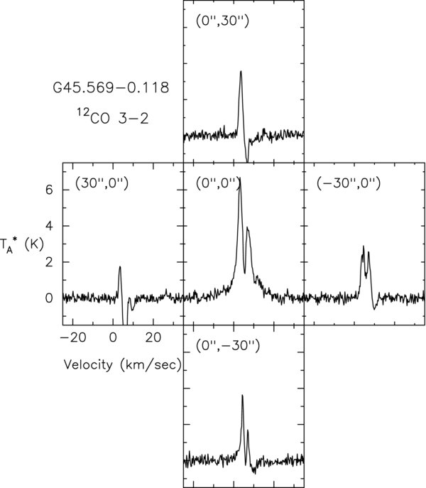
Figure 16. Example of the data obtained by observing the 12CO (3–2) emission. These data are for the position CO45.569 − 0.118 (see Table 5), chosen by visual inspection of an early version of the 850 μm continuum image, and not formally associated with any clump identified subsequently. The five positions observed are the center, and four points offset in the cardinal directions by 30'' (as indicated in each frame). The on-source central point shows the strongest emission, and also indications of a weak molecular outflow. The four off-source spectra show considerably weaker emission; all spectra show evidence of contamination from the reference position at a radial velocity (w.r.t. LSR) of about 7 km s−1.
Download figure:
Standard image High-resolution imageCO45.569 − 0.118 shows evidence of molecular outflow, with visible line wings at the central position extending to perhaps 20 km s−1 from the central velocity. Relatively few of the continuum clumps, however, have significant extended line wings resulting from outflowing gas, as is commonly found in star-forming cores. This is most likely because we selected against the more active star-forming regions by observing relatively weak continuum targets, for the most part. We identify the continuum clumps subsequently associated with the observed objects in Table 5. Eight of the original 12CO (3–2) targets were not ultimately selected by the automated continuum emission clump-finding technique, but nevertheless all show significant 12CO (3–2) emission apparently centered at the nominal continuum emission peak.
6. CALCULATION OF CLUMP MASSES
A determination of the masses of the dust clumps we have observed requires that the distance to each be known. For a given galactic longitude within the plane of the Galaxy, excepting the tangent point, there are two distances corresponding to a given velocity for each of the clumps identified in the 850 μm continuum observations. In principle, this dichotomy can be resolved by inspection of H i line data associated with each line of sight; the velocity of H i self-absorption (HISA) in the direction of each clump then indicates whether a particular molecular cloud (identified via 13CO (1–0) data from the GRS data) resides at the near or far distance. This technique was illustrated by Jackson et al. (2002) in the case of one region (GRSMS 45.6+0.3) included in the present work, and more recently further developed by others, e.g., Goldsmith & Li (2005). We show an example of the relation between the 13CO (1–0) GRS data and H i self-absorption in Figure 17 for one of the objects in the present work.
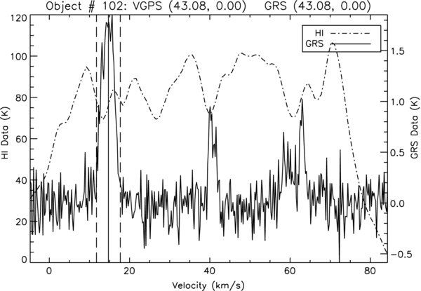
Figure 17. Example of the GRS/VGPS spectra used to resolve distance ambiguities for dust clumps; in this case for object 102 (G43.078+0.002; see Tables 2 and 6). The solid line shows the 13CO (1–0) spectrum, and the dot-dashed line traces the H i spectrum at the position of this object. The 13CO emission is related to H i self-absorption, the velocity of which places the associated dust clump at the far kinematic distance (11.1 kpc). This object appears to be associated with IRAS 19077+0856 (see Table 8).
Download figure:
Standard image High-resolution imageThe initial formal HISA processing for the 132 dust clumps was carried out by Alexis Johnson (during the tenure of a temporary student position at Boston University in 2007) using existing code developed for this purpose. Table 6 contains the results of this analysis; for each object (identified by its clump number in Table 6) we list the peak 13CO (1–0) intensity within the bounds of the clump at the emission match, the velocity of this emission, the determination of whether the emission is at the near (N) or far (F) distance, and the distance associated with this determination using the standard galactic rotation model. The "cloud number" given is the identifier obtained from the H i catalog maintained locally at Boston University. Individual clouds were assigned to either the near or far ("N" or "F") distance, in the final two columns of Table 6. A few clumps could not be positively identified with any particular cloud—these are therefore not assigned to a cloud number, do not have a near/far determination, and cannot be assigned a formal distance as a result. These objects are identified by zeros in the final three columns of Table 6. Some have associated low-level emission not associated with any cataloged cloud; others are best matched with negative-velocity components in the CfA longitude–velocity diagram; 13CO (1–0) data are not available for these velocities. In addition to the distance found for the larger associated H i cloud, distances for individual clumps within such clouds can also be estimated using the H i velocity observed at the location of the clump. We identify these two distances as the "cloud" and "clump" distances; based on the standard galactic rotation model, both are given in Table 6. While these distances are subject to the motions of the individual clumps in the Galaxy, we anticipate that they should be accurate to within 10%.
Table 6. Distance Determinations Obtained from 13CO (1–0) and H i Data
| Clumpa Number | Peakb 13CO (K) | Velocityc km s−1 | Clumpd N/F | Clumpe Distance (kpc) | Cloudf number | Cloudg N/F | Cloudh Distance (kpc) |
|---|---|---|---|---|---|---|---|
| 1 | 1.907 | 54.80 | F | 7.63 | 458 | F | 7.50 |
| 2 | 1.907 | 54.80 | F | 7.63 | 458 | F | 7.50 |
| 3 | 1.498 | 15.00 | N | 1.18 | 680 | N | 1.20 |
| 4 | 1.460 | 14.90 | N | 1.17 | 680 | N | 1.20 |
| 5 | 1.498 | 15.10 | N | 1.18 | 680 | N | 1.20 |
| 6 | 0.909 | 18.00 | N | 1.35 | 680 | N | 1.20 |
| 7 | 1.288 | 61.00 | F | 6.68 | 249 | F | 6.70 |
| 8 | 0.211 | 66.50 | F | 5.91 | 458 | F | 7.50 |
| 9 | 0.448 | 25.40 | F | 10.03 | 625 | F | 10.00 |
| 10 | 0.501 | 24.40 | F | 10.10 | 625 | F | 10.00 |
| 11 | 0.449 | 25.40 | F | 10.04 | 625 | F | 10.00 |
| 12 | 0.477 | 26.72 | F | 9.98 | 636 | F | 10.00 |
| 13 | 1.577 | 7.60 | F | 11.13 | 550 | F | 11.10 |
| 14 | 0.664 | 25.44 | F | 10.09 | 636 | F | 10.00 |
| 15 | 1.551 | 7.50 | F | 11.14 | 550 | F | 11.10 |
| 16 | 1.577 | 7.60 | F | 11.14 | 550 | F | 11.10 |
| 17 | 2.781 | 60.00 | F | 7.14 | 55 | F | 7.40 |
| 18 | 2.781 | 56.00 | F | 7.69 | 55 | F | 7.40 |
| 19 | 2.781 | 58.20 | F | 7.41 | 55 | F | 7.40 |
| 20 | 2.621 | 59.00 | F | 7.30 | 55 | F | 7.40 |
| 21 | 2.621 | 56.50 | F | 7.64 | 55 | F | 7.40 |
| 22 | 2.621 | 58.20 | F | 7.43 | 55 | F | 7.40 |
| 23 | 2.621 | 59.50 | F | 7.25 | 55 | F | 7.40 |
| 24 | 2.621 | 56.50 | F | 7.66 | 55 | F | 7.40 |
| 25 | 2.621 | 59.00 | F | 7.33 | 55 | F | 7.40 |
| 26 | 2.621 | 61.20 | F | 6.96 | 55 | F | 7.40 |
| 27 | 2.621 | 59.00 | F | 7.33 | 55 | F | 7.40 |
| 28 | 2.621 | 58.20 | F | 7.45 | 55 | F | 7.40 |
| 29 | 2.621 | 58.20 | F | 7.45 | 55 | F | 7.4 |
| 30 | 2.621 | 58.20 | F | 7.45 | 55 | F | 7.40 |
| 31 | 2.621 | 59.50 | F | 7.27 | 55 | F | 7.40 |
| 32 | 2.621 | 58.50 | F | 7.41 | 55 | F | 7.40 |
| 33 | 2.621 | 55.00 | F | 7.84 | 55 | F | 7.40 |
| 34 | 2.621 | 55.00 | F | 7.85 | 55 | F | 7.40 |
| 35 | 2.621 | 55.50 | F | 7.79 | 55 | F | 7.40 |
| 36 | 2.621 | 59.50 | F | 7.28 | 55 | F | 7.40 |
| 37 | 2.473 | 59.00 | N | 4.54 | 200 | N | 7.70 |
| 38 | 3.920 | 59.00 | N | 4.53 | 200 | N | 7.70 |
| 39 | 3.920 | 58.60 | N | 4.47 | 200 | N | 7.70 |
| 40 | 3.920 | 59.00 | N | 4.52 | 200 | N | 7.70 |
| 41 | 1.440 | 60.50 | N | 4.73 | 200 | N | 7.70 |
| 42 | 1.440 | 59.00 | N | 4.52 | 200 | N | 7.70 |
| 43 | 1.440 | 58.50 | N | 4.45 | 200 | N | 7.70 |
| 44 | 1.440 | 57.50 | N | 4.32 | 200 | N | 7.70 |
| 45 | 2.189 | 60.00 | F | 7.57 | 241 | F | 7.50 |
| 46 | 2.305 | 58.80 | F | 7.73 | 241 | F | 7.50 |
| 47 | 2.305 | 58.80 | F | 7.73 | 241 | F | 7.50 |
| 48 | 2.306 | 59.30 | F | 7.67 | 241 | F | 7.50 |
| 49 | 1.760 | 61.80 | F | 7.34 | 241 | F | 7.50 |
| 50 | 2.149 | 60.30 | F | 7.55 | 241 | F | 7.50 |
| 51 | 2.079 | 60.00 | F | 7.59 | 241 | F | 7.50 |
| 52 | 2.438 | 56.90 | N | 4.16 | 229 | N | 4.20 |
| 53 | 2.176 | 55.00 | N | 3.96 | 229 | N | 4.20 |
| 54 | 1.368 | 57.40 | N | 4.20 | 229 | N | 4.20 |
| 55 | 1.349 | 58.40 | N | 4.31 | 229 | N | 4.20 |
| 56 | 1.492 | 53.50 | N | 3.80 | 229 | N | 4.20 |
| 57 | 1.492 | 53.50 | N | 3.80 | 229 | N | 4.20 |
| 58 | 0.446 | 54.00 | N | 3.84 | 335 | N | 5.40 |
| 59 | 2.383 | 65.00 | N | 5.22 | 335 | N | 5.40 |
| 60 | 1.624 | 44.00 | F | 9.22 | 532 | F | 9.30 |
| 61 | 1.624 | 63.50 | N | 4.92 | 335 | N | 5.40 |
| 62 | 1.624 | 59.90 | N | 4.44 | 180 | N | 4.70 |
| 63 | 1.624 | 60.40 | N | 4.49 | 180 | N | 4.70 |
| 64 | 1.017 | 61.40 | N | 4.61 | 180 | N | 4.70 |
| 65 | 1.017 | 67.50 | N | 5.91 | 0 | 0 | 0.00 |
| 66 | 1.017 | 43.00 | N | 2.93 | 376 | N | 2.70 |
| 67 | 1.017 | −15.00 | N | 6.14 | 0 | 0 | 0.00 |
| 68 | 0.687 | −15.00 | N | 6.14 | 0 | 0 | 0.00 |
| 69 | 0.816 | 66.00 | N | 5.32 | 180 | N | 4.70 |
| 70 | 0.452 | −15.00 | F | 6.16 | 0 | 0 | 0.00 |
| 71 | 1.466 | 61.00 | N | 4.52 | 180 | N | 4.70 |
| 72 | 0.452 | −15.00 | F | 6.16 | 0 | 0 | 0.00 |
| 73 | 1.517 | 61.40 | N | 4.56 | 180 | N | 4.70 |
| 74 | 0.722 | 65.40 | F | 7.21 | 381 | F | 7.30 |
| 75 | 0.564 | −15.00 | F | 6.17 | 0 | 0 | 0.00 |
| 76 | 0.722 | 65.40 | F | 7.22 | 381 | F | 7.30 |
| 77 | 1.502 | 60.40 | N | 4.43 | 180 | N | 4.70 |
| 78 | 1.502 | 59.80 | N | 4.35 | 520 | N | 4.10 |
| 79 | 1.502 | 60.00 | N | 4.37 | 520 | N | 4.10 |
| 80 | 1.502 | 64.40 | F | 7.45 | 381 | F | 7.30 |
| 81 | 1.502 | 12.30 | F | 11.38 | 94 | F | 11.40 |
| 82 | 1.502 | 12.80 | F | 11.36 | 94 | F | 11.40 |
| 83 | 1.502 | 6.80 | F | 11.70 | 94 | F | 11.40 |
| 84 | 1.502 | 6.80 | F | 11.70 | 94 | F | 11.40 |
| 85 | 1.502 | 11.80 | F | 11.42 | 94 | F | 11.40 |
| 86 | 1.144 | 11.80 | F | 11.43 | 94 | F | 11.40 |
| 87 | 1.144 | 11.80 | F | 11.43 | 94 | F | 11.40 |
| 88 | 1.144 | 60.20 | N | 4.38 | 520 | N | 4.10 |
| 89 | 1.144 | 11.80 | F | 11.43 | 94 | F | 11.40 |
| 90 | 1.144 | 10.00 | F | 11.53 | 94 | F | 11.40 |
| 91 | 1.144 | 12.00 | F | 11.42 | 94 | F | 11.40 |
| 92 | 1.144 | 8.80 | F | 11.60 | 94 | F | 11.40 |
| 93 | 1.144 | 12.00 | F | 11.43 | 94 | F | 11.40 |
| 94 | 1.144 | 12.30 | F | 11.41 | 94 | F | 11.40 |
| 95 | 1.144 | 13.80 | F | 11.33 | 94 | F | 11.40 |
| 96 | 1.144 | 9.00 | F | 11.60 | 94 | F | 11.40 |
| 97 | 1.144 | 12.30 | F | 11.42 | 94 | F | 11.40 |
| 98 | 1.144 | 3.00 | F | 11.93 | 94 | F | 11.40 |
| 99 | 1.144 | 12.80 | F | 11.39 | 94 | F | 11.40 |
| 100 | 1.144 | 3.00 | F | 11.94 | 94 | F | 11.40 |
| 101 | 1.144 | 15.00 | F | 11.27 | 708 | F | 11.10 |
| 102 | 1.144 | 14.50 | F | 11.30 | 708 | F | 11.10 |
| 103 | 1.144 | 13.50 | F | 11.35 | 708 | F | 11.10 |
| 104 | 1.144 | 14.50 | F | 11.30 | 708 | F | 11.10 |
| 105 | 1.144 | 8.80 | F | 11.63 | 94 | F | 11.40 |
| 106 | 1.144 | 8.50 | F | 11.65 | 94 | F | 11.40 |
| 107 | 0.883 | 8.50 | F | 11.67 | 94 | F | 11.40 |
| 108 | 1.059 | 57.00 | N | 4.03 | 238 | N | 4.80 |
| 109 | 0.883 | 8.50 | F | 11.67 | 94 | F | 11.40 |
| 110 | 0.942 | 58.00 | N | 4.12 | 238 | N | 4.80 |
| 111 | 1.253 | 66.00 | N | 5.05 | 238 | N | 4.80 |
| 112 | 1.759 | 66.00 | N | 5.03 | 238 | N | 4.80 |
| 113 | 1.754 | 64.90 | N | 4.87 | 238 | N | 4.80 |
| 114 | 0.999 | 62.10 | N | 4.53 | 238 | N | 4.80 |
| 115 | 1.759 | 66.10 | N | 5.04 | 238 | N | 4.80 |
| 116 | 1.724 | 65.10 | N | 4.89 | 238 | N | 4.80 |
| 117 | 1.032 | 57.75 | N | 4.08 | 520 | N | 4.10 |
| 118 | 0.464 | 67.10 | N | 5.19 | 520 | N | 4.10 |
| 119 | 0.464 | 58.00 | F | 8.42 | 420 | F | 7.70 |
| 120 | 0.464 | 65.40 | F | 7.60 | 420 | F | 7.70 |
| 121 | 0.464 | 58.00 | F | 8.44 | 0 | 0 | 0.00 |
| 122 | 0.464 | 64.40 | F | 7.78 | 420 | F | 7.70 |
| 123 | 0.464 | 65.40 | F | 7.66 | 420 | F | 7.70 |
| 124 | 0.464 | 62.40 | F | 8.02 | 420 | F | 7.70 |
| 125 | 0.464 | 64.40 | F | 7.79 | 420 | F | 7.70 |
| 126 | 0.464 | 64.40 | F | 7.79 | 420 | F | 7.70 |
| 127 | 2.072 | 63.40 | F | 7.92 | 420 | F | 7.70 |
| 128 | 2.072 | 62.40 | F | 8.03 | 420 | F | 7.70 |
| 129 | 2.072 | 65.40 | F | 7.67 | 420 | F | 7.70 |
| 130 | 1.517 | 56.30 | N | 3.92 | 452 | N | 4.00 |
| 131 | 1.496 | 55.50 | F | 8.72 | 420 | F | 7.70 |
| 132 | 1.533 | 27.60 | N | 1.88 | 724 | N | 1.90 |
Notes. aClump number (as in Table 2). bPeak 13CO 1–0 intensity. cVelocity w.r.t. local standard of rest. dNear/Far (N/F) clump distance resolution. eDistance based on clump velocity. fH i catalogue cloud number. gNear/Far (N/F) distance resolution based on H i cloud data. hDistance derived from H i cloud data.
Subsequent comparison of the subset of the HISA results with those for which there are also JCMT 12CO and 13CO (3–2) data (55 clumps in total) revealed that the velocity determinations obtained from the latter substantially differed in 11 of these objects. In four of these cases the HISA analysis found no suitable velocity match; these objects appear in Table 6 with an assigned velocity of −15 km s−1. In light of this issue the H i and 13CO (1–0) spectra of this group of sources were re-examined by Julia Duval (Boston University), using the 12CO (3–2) velocity obtained from the JCMT data. In all cases 13CO (1–0) emission could be identified at the same velocity as observed in the 12CO (3–2) line. We then used H i self-absorption data obtained from the VLA Galactic Plane Survey (Stil et al. 2008) to search for H i self-absorption in order to resolve the near/far kinematic distance dichotomy obtained from the Clemens galactic rotation curve.
From the "cloud" and "clump" distance data in Table 6 we derive two estimates of the clump masses Mclump, using the relation (see, e.g., Johnstone et al. 2001)
where we assume that the emission arises in optically thin dust particles having a dust temperature Td and a dust opacity κ850 = 0.02 cm2 gm−1. We further assume that the dust has a typical temperature Td ∼ 15 K, based on results obtained from other investigations of the physical properties of infrared-dark clouds (Egan et al. 1998; Carey et al. 1998; Johnstone et al. 2003). Based on our estimates for the uncertainties in the flux density and distance scales of 20% and 10% respectively, formula 1 above suggests that the masses we derive are uncertain by a factor of approximately 2.
These cloud/clump mass data are summarized in Table 7. In a few cases (7 of 132 in total) we were unable to determine a value for the "cloud" distance, and only the "clump" distance allows us to derive a value for the mass. Since the masses determined using the "cloud" and "clump" distances are very similar in objects where both values have been determined, we conclude that for the few clumps where only a "clump" distance is available, the associated mass estimate is reasonable.
Table 7. Clump Masses Based on Clump and Cloud Distance Determinations
| Clump Number | Mclpa (M☉) | Mcldb (M☉) | Clump Number | Mclpa (M☉) | Mcldb (M☉) | Clump Number | Mclpa (M☉) | Mcldb (M☉) | Clump Number | Mclpa (M☉) | Mcldb (M☉) |
|---|---|---|---|---|---|---|---|---|---|---|---|
| 1 | 1720.0 | 1660.0 | 34 | 601.0 | 536.0 | 67 | 261.0 | ⋅⋅⋅ | 100 | 1860.0 | 1700.0 |
| 2 | 523.0 | 505.0 | 35 | 1140.0 | 1030.0 | 68 | 54.0 | ⋅⋅⋅ | 101 | 1320.0 | 1280.0 |
| 3 | 10.0 | 10.4 | 36 | 358.0 | 370.0 | 69 | 476.0 | 371.0 | 102 | 1600.0 | 1540.0 |
| 4 | 26.4 | 27.8 | 37 | 34.8 | 100.0 | 70 | 77.6 | ⋅⋅⋅ | 103 | 2770.0 | 2650.0 |
| 5 | 5.6 | 5.8 | 38 | 339.0 | 981.0 | 71 | 374.0 | 405.0 | 104 | 954.0 | 920.0 |
| 6 | 32.1 | 25.4 | 39 | 5720.0 | 16700.0 | 72 | 67.5 | ⋅⋅⋅ | 105 | 758.0 | 728.0 |
| 7 | 496.0 | 499.0 | 40 | 342.0 | 991.0 | 73 | 325.0 | 346.0 | 106 | 809.0 | 774.0 |
| 8 | 258.0 | 415.0 | 41 | 169.0 | 448.0 | 74 | 180.0 | 185.0 | 107 | 460.0 | 439.1 |
| 9 | 1570.0 | 1560.0 | 42 | 267.0 | 775.0 | 75 | 152.0 | ⋅⋅⋅ | 108 | 53.4 | 75.8 |
| 10 | 943.0 | 925.0 | 43 | 2870.0 | 8590.0 | 76 | 227.0 | 232.0 | 109 | 436.0 | 416.0 |
| 11 | 350.0 | 347.0 | 44 | 78.0 | 248.0 | 77 | 155.0 | 175.0 | 110 | 57.4 | 77.9 |
| 12 | 523.0 | 525.0 | 45 | 280.0 | 275.0 | 78 | 261.0 | 232.0 | 111 | 138.0 | 125.0 |
| 13 | 1040.0 | 1030.0 | 46 | 1270.0 | 1200.0 | 79 | 1310.0 | 1150.0 | 112 | 83.2 | 75.8 |
| 14 | 1320.0 | 1300.0 | 47 | 563.0 | 530.0 | 80 | 1020.0 | 976.0 | 113 | 48.5 | 47.1 |
| 15 | 3590.0 | 3560.0 | 48 | 1030.0 | 980.0 | 81 | 541.0 | 543.0 | 114 | 51.1 | 57.4 |
| 16 | 1160.0 | 1150.0 | 49 | 493.0 | 515.0 | 82 | 677.0 | 682.0 | 115 | 85.8 | 77.9 |
| 17 | 277.0 | 297.0 | 50 | 405.0 | 400.0 | 83 | 13800.0 | 13100.0 | 116 | 434.0 | 418.0 |
| 18 | 1050.0 | 974.0 | 51 | 318.0 | 310.0 | 84 | 2620.0 | 2480.0 | 117 | 117.0 | 118.0 |
| 19 | 1090.0 | 1091.0 | 52 | 1390.0 | 1410.0 | 85 | 1740.0 | 1730.0 | 118 | 67.1 | 41.9 |
| 20 | 569.0 | 584.0 | 53 | 506.0 | 569.0 | 86 | 430.0 | 428.0 | 119 | 214.0 | 179.3 |
| 21 | 327.0 | 307.0 | 54 | 31.4 | 31.4 | 87 | 2210.0 | 2200.0 | 120 | 318.0 | 327.0 |
| 22 | 133.0 | 131.0 | 55 | 121.0 | 115.0 | 88 | 58.0 | 50.8 | 121 | 532.0 | ⋅⋅⋅ |
| 23 | 3200.0 | 3340.0 | 56 | 88.6 | 108.0 | 89 | 41500.0 | 41300.0 | 122 | 694.0 | 680.0 |
| 24 | 835.0 | 779.0 | 57 | 75.8 | 92.5 | 90 | 279000.0 | 273000.0 | 123 | 1520.0 | 1540.0 |
| 25 | 330.0 | 336.0 | 58 | 119.0 | 236.0 | 91 | 58000.0 | 57800.0 | 124 | 183.0 | 169.0 |
| 26 | 5260.0 | 5950.0 | 59 | 671.0 | 718.0 | 92 | 34700.0 | 33500.0 | 125 | 1338.0 | 1310.0 |
| 27 | 8110.0 | 8270.0 | 60 | 1060.0 | 1080.0 | 93 | 2510.0 | 2500.0 | 126 | 281.0 | 274.0 |
| 28 | 948.0 | 935.0 | 61 | 200.0 | 241.0 | 94 | 359.0 | 358.0 | 127 | 145.0 | 137.0 |
| 29 | 8550.0 | 8430.0 | 62 | 119.0 | 134.0 | 95 | 251.0 | 254.0 | 128 | 229.0 | 211.0 |
| 30 | 2290.0 | 2260.0 | 63 | 258.0 | 283.0 | 96 | 4310.0 | 4160.0 | 129 | 126.0 | 127.0 |
| 31 | 616.0 | 638.0 | 64 | 161.0 | 167.0 | 97 | 1930.0 | 1918.0 | 130 | 62.9 | 65.4 |
| 32 | 879.0 | 876.0 | 65 | 124.0 | ⋅⋅⋅ | 98 | 481.0 | 439.0 | 131 | 534.0 | 416.0 |
| 33 | 978.0 | 872.0 | 66 | 1220.0 | 1040.0 | 99 | 2030.0 | 2030.0 | 132 | 113.0 | 115.0 |
Notes. aClump mass derived from the clump distance as listed in Table 6. bClump mass derived from the cloud distance as listed in Table 6.
Download table as: ASCIITypeset image
The fractional uncertainty in clump mass can in turn be determined from the cloud distance and the uncertainty in the flux density. The latter provides the primary source of error, which we estimate is about 20%. Secondary sources of error arise from the dust opacity assumed, which is likely to vary by at least a factor of 2, and may well vary significantly across the range of clump properties included in this work. In combination with the uncertainty in the distances of individual clumps (at least 10%), it is clear that clump properties (in particular, mass) cannot be very precisely determined.
From the clump masses, one can compute the mass function of dust clumps within the observed region of the Galactic Plane. The cumulative mass function, N(M), is usually parameterized as a power law with N(M) ∝ M−α. When α < 1, the bulk of the mass resides in the largest clumps. Alternatively, when α>1 the bulk of the mass resides in the smallest clumps. Thus, the Salpeter (1955) mass function for stars, with α = 1.35, puts most of the stellar mass in low-mass stars. For cores in nearby molecular clouds, observed in the submillimeter wavelength regime a similarly large value for α has been measured (e.g., Motte et al. 1998; Johnstone et al. 2000; Alves et al. 2007). At larger distances, however, the mass function of submillimeter clumps is much more ambiguous (e.g., Reid & Wilson 2006; Rathborne et al. 2006; Ragan et al. 2009).
Figure 18 depicts the distribution of dust mass versus radius for all the clumps identified in the present data at 850 μm. The dash-dotted line denotes the mean surface brightness sensitivity of the survey; below this line clumps are too faint to be detected. A majority of the identified clumps with mass below 500 M☉ are near the observational sensitivity limit, which suggests that substantial incompleteness may begin well before the threshold for detection is reached. Thus, cumulative mass plots, such as those in Figure 18, should be interpreted with caution. The solid line shows where gravity is balanced by thermal pressure. This indicates that all of the clumps identified would require additional support (e.g., via nonthermal motions or magnetic fields) in order to avoid gravitational collapse. This situation holds even for rather higher temperatures than we have assumed in this work (15 K). The dashed line shows where gravity is balanced by the typical nonthermal motions observed around each clump (using the mean CO line width of 4 km s−1 FWHM).
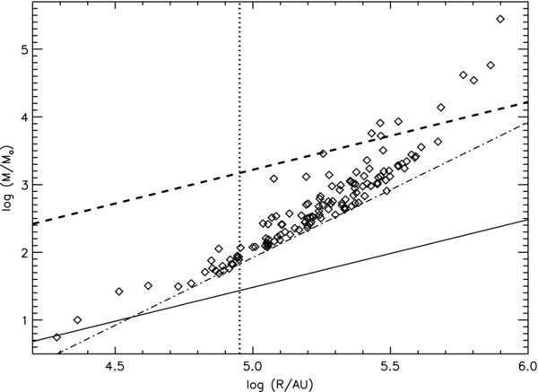
Figure 18. Distribution of the masses of the dust clumps, plotted as a function of radius, using the distances given in Table 6. The dash-dot line shows the minimum observational sensitivity to mass as a function of clump radius, while the vertical dotted line indicates the minimum resolvable clump size at the largest distance range. The solid line shows virial equilibrium for objects with a temperature of 15 K (as assumed for the calculation of the clump masses). The dashed line shows virial equilibrium for objects with a nonthermal line width of 4 km s−1 FWHM.
Download figure:
Standard image High-resolution image7. 12CO (3–2) AND 850 μm EMISSION
It is to be expected that there should be a relationship between the 850 μm flux density and the 12CO (3–2) emission, and for those objects where we have mapping data in the 13CO (3–2) line, this is confirmed. The continuum emission at these wavelengths is optically thin, and thus the flux density scales directly to the dust mass within the beam. For low optical depths, the 12CO and 13CO (3–2) should also exhibit the same behavior, assuming a constant gas-dust ratio. In more extreme circumstances, at very low densities the dust may well be evaporated by stellar radiation, and the relationship would break down. At higher densities the emission from 12CO (3–2) rapidly becomes optically thick with increasing column density, while the 13CO (3–2) line emission remains optically thin to much greater associated continuum column densities. Furthermore, it is highly probable that a significant fraction of the CO contained within these clumps is simply invisible, being frozen out at the low temperatures (we use 15 K in the absence of more complete data) expected in cores, in particular those which do not contain stars. We cannot reliably predict the degree to which this might be occurring in the sample of objects we have examined in this work.
We use the present limited 12CO and 13CO (3–2) observations to illustrate this point, by comparing the peak 850 μm flux density for those clumps for which we obtained molecular line data. We show the results in Figure 19. The 13CO (3–2) data, shown in the frame to the right, exhibit a linear relationship within the probable errors over the range of continuum flux densities up to 10 Jy beam−1. The 12CO data, at left, also indicate a linear relationship with the continuum flux density, but the relationship breaks down at quite low flux densities, probably at less than 2 Jy beam−1.
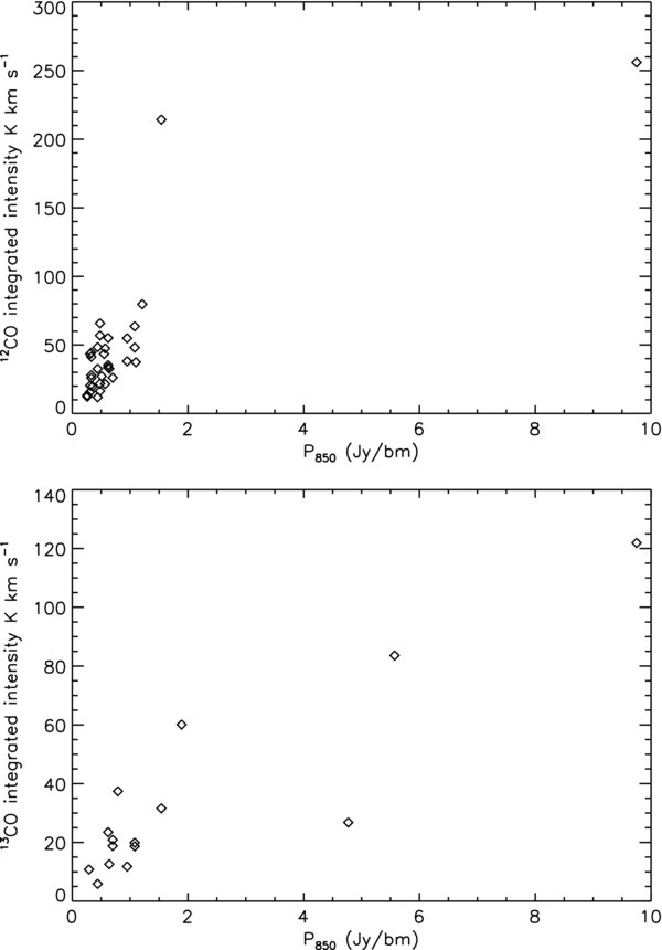
Figure 19. Comparison of the 12CO (at left) and 13CO 3-2 (right) integrated intensities with the 850 μm flux density for objects observed in this program. The majority of the objects were not observed in both CO transitions, with the exception of the strongest source, corresponding to the clump G43.706-0.169.
Download figure:
Standard image High-resolution imageIn this paper, we employ the 13CO (1–0) GRS data as the primary means to obtain kinematic distances of the continuum sources in this part of the Galaxy, if the line and continuum emission can be associated with the same object. However, the 13CO (1–0) transition tends to emphasize relatively cool, more diffuse, material, whereas the millimeter and submillimeter continuum emission arises in compact regions with relatively high column density. Furthermore, the observing beam sizes for the 13CO (1–0) and the 850 μm data sets are substantially different. For these reasons we cannot always be entirely sure of the physical relationship between a given continuum feature and an object seen in the spectral line data.
The 850 μm image shown earlier in Figure 11 also illustrates this point. While there is generally a good correspondence between the continuum emission clumps in the images and structures in the 13CO (1–0) survey data, the converse is not true; there are a number of 13CO features which do not appear in the continuum data. This may be simply a result of the limited sensitivity of the continuum images, or it may be that the dust/gas ratio diminishes when the optical depth in the cloud is relatively low, perhaps due to evaporation of grains due to incident starlight.
8. COMPARISONS WITH OTHER SURVEY DATA SETS
8.1. The Physical Content of Dust Clumps
In order to investigate the nature and range of environments of the dust clumps found in the present small-scale survey, we made use of the Simbad online search engine.14 For each dust clump in Table 2 we searched within a radius of 1' for associated objects. The results of this endeavor are contained in Table 8. Approximately half (64) of the 132 clumps detected at 850 μm are associated with other previously cataloged sources of emission on the basis of this search. Most of the objects identified are characteristic of star-forming regions, exhibiting infrared emission (e.g., IRAS and MSX sources), thermal radio or submillimeter-wavelength emission, maser activity in spectral lines of OH, H2O and CH3OH, and stellar components. However, some caution is needed in assigning associated emission with the cold dust clumps found in this work. In particular, the IRAS catalog positions are quite imprecise when compared with the current work, as are those to be found in a number of the older catalogs.
Table 8. Sources of Emission Probably Associated with Dust Clumps
| Clump | Associationsa |
|---|---|
| 1 | IRAS 19120+1148 |
| 2 | IRAS 19120+1148 |
| 3 | RRF 353 |
| 4 | IRAS 19125+1142 |
| 5 | RRF 353 |
| 6 | MSX6C G046.0599+00.2240 |
| 7 | ⋅⋅⋅ |
| 8 | ⋅⋅⋅ |
| 9 | IRAS 19124+1131 |
| 10 | ⋅⋅⋅ |
| 11 | ⋅⋅⋅ |
| 12 | ⋅⋅⋅ |
| 13 | ⋅⋅⋅ |
| 14 | IRAS 19116+1120 |
| 15 | ⋅⋅⋅ |
| 16 | ⋅⋅⋅ |
| 17 | ⋅⋅⋅ |
| 18 | ⋅⋅⋅ |
| 19 | IRAS 19124+1106, GPSR 45.543-0.007 |
| 20 | ⋅⋅⋅ |
| 21 | ⋅⋅⋅ |
| 22 | ⋅⋅⋅ |
| 23 | MSX5C G045.4780+00.1322; CH3OH 045.49+00.13 |
| 24 | MSX6C G045.4658+00.0457; H2O 045.46+00.05 |
| 25 | ⋅⋅⋅ |
| 26 | MSX5C G045.4780+00.1322; GAL 045.48+00.13 |
| 27 | Caswell OH 045.47+00.05 GAL 045.5+00.0 |
| 28 | Caswell CH3OH 045.47+00.05; MSX6C G045.4658+00.0457 |
| 29 | MSX5C G045.4542+00.0600; G045.455+0.060 |
| 30 | GAL 045.5+00.0: GRSMC 45.46+0.05 |
| 31 | Caswell CH3OH 045.44+00.07; GAL 045.47+00.05 |
| 32 | Caswell OH 045.466+00.045 |
| 33 | GRS 045.40+00.10; Caswell H2O 045.44+00.07 |
| 34 | SNR G045.5+00.1 |
| 35 | ⋅⋅⋅ |
| 36 | ⋅⋅⋅ |
| 37 | ⋅⋅⋅ |
| 38 | GPA 045.16+0.11(radio source) |
| 39 | Caswell OH 045.12+00.13,MSX6C G045.1221+00.1323 |
| 40 | RRF 342 (radio source) |
| 41 | ⋅⋅⋅ |
| 42 | GRS 045.07 +00.14, GAL 045.1+00.1 (H ii region) |
| 43 | G45.07+0.13 1 (maser); KJK G45.07 1 (IR) |
| 44 | KJK G45.07 3 (IR source) |
| 45 | IRAS 19110+1007; RFS 765 (Radio-source) |
| 46 | PSR B1910+10.1 (pulsar) |
| 47 | ⋅⋅⋅ |
| 48 | ⋅⋅⋅ |
| 49 | ⋅⋅⋅ |
| 50 | ⋅⋅⋅ |
| 51 | ⋅⋅⋅ |
| 52 | MSX6CG044.3103+00.0416; IRAS 19098+1002 |
| 53 | ⋅⋅⋅ |
| 54 | IRAS 19092+1004 |
| 55 | ⋅⋅⋅ |
| 56 | ⋅⋅⋅ |
| 57 | ⋅⋅⋅ |
| 58 | [HLB98] Onsala 100 (maser) |
| 59 | HaroChavira 56 (star) |
| 60 | IRAS 19097+0941 |
| 61 | IRAS 19088+0943 |
| 62 | ⋅⋅⋅ |
| 63 | ⋅⋅⋅ |
| 64 | ⋅⋅⋅ |
| 65 | ⋅⋅⋅ |
| 66 | G043.796-00.127 (maser); G043.80-00.13 (sub-mm source) |
| 67 | ⋅⋅⋅ |
| 68 | IRAS 19084+0935 |
| 69 | IRAS 19094+0924 |
| 70 | ⋅⋅⋅ |
| 71 | IRAS 19085+0920 |
| 72 | ⋅⋅⋅ |
| 73 | IRAS 19085+0920 |
| 74 | ⋅⋅⋅ |
| 75 | ⋅⋅⋅ |
| 76 | IRAS 19079+0919 |
| 77 | ⋅⋅⋅ |
| 78 | ⋅⋅⋅ |
| 79 | IRAS 19088+0902; [CF95]39 (maser) |
| 80 | ⋅⋅⋅ |
| 81 | ⋅⋅⋅ |
| 82 | ⋅⋅⋅ |
| 83 | IRAS 19081+0903, G043.24-00.05 (sub-mm) |
| 84 | GAL 043.23-00.05 (H ii region); GPSR 43.237-0.045 (radio source) |
| 85 | 043.2+00.0 (unknown nature) |
| 86 | ⋅⋅⋅ |
| 87 | ⋅⋅⋅ |
| 88 | BD+08 3994 (star); IRAS 19085+0855 |
| 89 | W49 JJ (radio source); GAL 043.2-00.0 (molecular cloud) |
| 90 | W49 B,D,E (H ii regions);GAL 043.17+00.01 (IR source) |
| 91 | G043.165-00.028 (Maser); W49A South (H ii region) |
| 92 | W49 R3 (Radio source); MSX5C G043.1485+00.0126 (IR) |
| 93 | ⋅⋅⋅ |
| 94 | ⋅⋅⋅ |
| 95 | ⋅⋅⋅ |
| 96 | OH 43.13 +0.04 (maser) |
| 97 | ⋅⋅⋅ |
| 98 | ⋅⋅⋅ |
| 99 | ⋅⋅⋅ |
| 100 | ⋅⋅⋅ |
| 101 | IRAS 19077+0856 |
| 102 | IRAS 19077+0856 |
| 103 | ⋅⋅⋅ |
| 104 | ⋅⋅⋅ |
| 105 | IRAS 19076+0852 |
| 106 | ⋅⋅⋅ |
| 107 | ⋅⋅⋅ |
| 108 | ⋅⋅⋅ |
| 109 | ⋅⋅⋅ |
| 110 | IRAS 19077+0839 |
| 111 | ⋅⋅⋅ |
| 112 | ⋅⋅⋅ |
| 113 | ⋅⋅⋅ |
| 114 | IRAS 19075+0832 |
| 115 | ⋅⋅⋅ |
| 116 | ⋅⋅⋅ |
| 117 | IRAS 19076+0827 |
| 118 | ⋅⋅⋅ |
| 119 | IRAS 19073+0826; WSRTGP 1907+0826 (radio source) |
| 120 | IRAS 19073+0825 |
| 121 | ⋅⋅⋅ |
| 122 | ⋅⋅⋅ |
| 123 | GAL 042.44-00.26 (H ii region); 042.435-0.260 (radio source) |
| 124 | WSRTGP 1907+0814 (radio-source); GAL 042.44-00.26 (H ii region) |
| 125 | Onsala 97 (maser); 042.42-0.27; H ii region |
| 126 | (as for object 125) |
| 127 | ⋅⋅⋅ |
| 128 | ⋅⋅⋅ |
| 129 | ⋅⋅⋅ |
| 130 | ⋅⋅⋅ |
| 131 | IRAS 19070+0811 |
| 132 | IRAS 19072+0806 |
Note. aOther sources of emission probably associated with this dust clump, within a radius of 1 arcmin from the dust clump position.
Overall, data from the InfraRed Astronomical Satellite Point Source Catalog (IRAS-PSC) show that there are an average of about 55 far-infrared sources per square degree within an area of about 25 deg2 surrounding the present region observed with SCUBA and SIMBA. As a group IRAS objects are essentially uniformly distributed on this scale, a result of the large extragalactic contribution to the data set. About 120 of these objects lie within the boundary of the SCUBA image. Using the GAIA display tool as an alternative approach, we visually examined an overlay of the two data sets for correspondences between these and 850 μm emission clumps in order to accommodate the lower positional accuracy of the IRAS-PSC images (about 20'') and the larger beam size (about 30'' at 12 μm) relative to the SCUBA data. We found that 39 IRAS objects are potentially associated with dust clumps observed at 850 μm. These objects show a marked preference for association with the brighter 850 μm clumps, as would be expected for star-forming clouds. The larger beamwidth of the IRAS data does not allow us to distinguish multiple cold dust components obtained from the clump-finding analysis within complex regions such as W49.
8.2. Spitzer Images
Data from the Spitzer satellite in particular are of considerable interest in the context of the current work. In a subsequent paper we intend to discuss the present results in light of the 24 μm images from this instrument. For the present, we show two small sections each about 12' square of the field which contain interesting extended structures at the millimeter and submillimeter wavelengths.
The first of these, in Figure 20, shows an object which has an apparent head-tail structure more clearly seen in the 1200 μm image. The single millimeter and submillimeter wavelength clump in the field is seen at 24 μm, and there is evidence at the mid-IR wavelength of associated structure in the region of the tail. Based on the CO velocity, we estimate this object (G45.651 + 0.272) to lie at a distance of about 10 kpc (see Table 6).
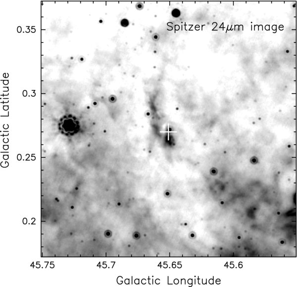
Figure 20. 24 μm image of a region 12' square centered on the 850/1200 μm object G45.651+0.272 (at the position of the cross), also coincident within the errors with IRAS 19116+1120. This position marks the "head" of an apparent head-tail submillimeter continuum structure extending to the north, also visible at 24 μm. In this and the next figure individual star images show the Multiband Imaging Photometer for Spitzer 24 μm instrumental diffraction pattern (Engelbracht et al. 2007)—in most cases this appears as a simple diffraction ring; however, for the brightest stars additional features appear, with hexagonal symmetry arising from the primary and secondary mirrors, while the brightest stars result in 12-fold dotted symmetry and six-fold vanes.
Download figure:
Standard image High-resolution imageThe second object for which we have Spitzer data is the "ridge" of emission centered at about G44.48 − 0.13 (see also the discussion in Section 4.1 and Figures 12 and 13). This consists of about six clumps of millimeter and submillimeter emission, in which the structure is clearly seen at both 850 and 1200 μm. The velocity w.r.t. the LSR for all these clumps is about 60 km s−1, and we conclude that these objects are part of a coherent structure. In this case, the 24 μm image (see Figure 21) shows no obvious counterparts to the millimeter and submillimeter wavelength images; however, a bright stellar object lies off the eastern extremity of the submillimeter wavelength ridge; this object corresponds to IRAS 19110+1007.
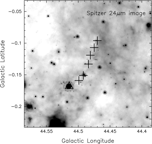
Figure 21. Image obtained by the Spitzer Space Telescope, showing the locations (at the crosses) of six clumps of submillimeter emission which appear to be part of a coherent structure, based on their very similar radial velocities (see Table 3). None of these objects have counterparts at 24 μm, although a pulsar (see Table 8) is coincident within the positional errors with the dust clump G44.499 − 0.158 at the southern extremity. An IRAS object is nearby, at the southern extremity of the emission ridge (at the position of the triangle); no cold dust emission was detected at this position.
Download figure:
Standard image High-resolution image
9. CONCLUSIONS
We have presented the results of parallel efforts to obtain relatively large-scale millimeter and submillimeter wavelength images of continuum emission from cold dust in a section of the Galactic plane 2 deg2 in extent, toward ℓ ∼ 44° ± 2°, using complementary chop-scanning and Fastscanning techniques.
The observed emission from the present region, typical of star-forming clouds in the Galaxy, is strongly clumped. 132 dust clumps were identified, and using distances for these objects derived from CO emission and H i self-absorption data we find that they range in mass from a few M☉ to almost 3 × 10⁵ M☉. We find that the cumulative mass spectral index of these objects is about unity over those distance bins which contain sufficient clumps for a determination. We note also that, for the assumed dust temperature of 15 K, the clumps are too massive to be supported by thermal pressure alone, and hence one can expect that such clouds will naturally form star clusters via fragmentation and subsequent collapse of the individual fragments.
The present observations are a fairly small effort to gain some insight into the behavior of large dust concentrations which are expected to collapse under self-gravity into star-forming clumps. Much more extensive surveys of the submillimeter wavelength continuum emission sky are planned by various groups using the JCMT once the next-generation imaging receiver SCUBA2 becomes fully operational in the near future.
We are grateful to the staff of the JCMT and to various visiting observers at the telescope for assistance in carrying out the 850 μm observations under the flexible service observing scheme. In particular, we thank the telescope operators for their fine attention to detail during the observing periods. We also greatly appreciate the efforts made by local staff during the latter half of this program to maintain SCUBA in working condition at a time when the instrument was having operational difficulties.
The JCMT observations were obtained during the execution of a joint Canada–UK project under programs M03BU18, M04AC15, S04BC11, and M05BC11. The JCMT is operated by the Joint Astronomy Centre, on behalf of the Science and Technology Facilities Council of the United Kingdom, the Netherlands Organization for Scientific Research, and the National Research Council of Canada. The SEST observations made use of SIMBA, a 37-element bolometer array, and the observing program was carried out on site in Chile by several of the co-authors of the present paper.
We are indebted to Alexis Johnson and Julia Duval (formerly term assistants at Boston University) for providing us with distance estimates based on H i self-absorption and 13CO (1–0) data, and for the resolution of problematic cases of disagreement between the CO (1–0) and (3–2) velocities. In addition, we thank Ronak Shah, also formerly at Boston University, for his assistance with processing images from the Boston University/FCRAO Galactic Ring Survey (GRS) data.
We also thank the anonymous referee for providing detailed and helpful comments, which resulted in a substantially improved paper over that originally submitted.
This publication makes use of molecular line data from the Boston University-FCRAO Galactic Ring Survey (GRS). The GRS is a joint project of Boston University and Five College Radio Astronomy Observatory, funded by the National Science Foundation under grants AST-9800334, AST-0098562, and AST-0100793.
Helen Kirk was supported by NSERC CGSD and NRC GSSSP awards (Canada). Doug Johnstone is supported by a Natural Sciences and Engineering Research Council of Canada grant.
Finally, we acknowledge the following organizations and facilities. The National Radio Astronomy Observatory is a facility of the National Science Foundation operated under cooperative agreement by Associated Universities, Inc. GAIA was developed by the Starlink Project and funded by the Particle Physics and Astronomy Research Council (UK). It is a derivative of the SkyCat image display and catalogue browsing tool, developed as part of the VLT project at ESO.
APPENDIX: PREPARATORY OBSERVATIONS OF G34.3+0.2
Prior to obtaining the data presented in this work, we made 850 μm observations with SCUBA at JCMT in 2000 to verify system performance and test our observational procedures. For this, we imaged a region centered on the strong continuum source G34.3+0.2, using the same parameters as we planned to use for individual sections of the Galactic Plane survey (see Section 2.1.1). The results of these observations are presented in Figure 1. The data were reduced using the same procedures as for the 16 individual fields which constitute the JCMT observations in this paper.
Although G34.3+0.2 is frequently used as a calibrator at millimeter and submillimeter wavelengths, there are rather few observations which provide images of the continuum emission from the region on the larger scale. One of the earliest observations of the region obtained with SCUBA imaged the central 2 arcmin (Strong-Jones et al. 1991). At the center of G34.3+0.2 is a cometary nebula which has been imaged at radio wavelengths on arcsecond scales (e.g., van Buren et al. 1990). Our observations show the structure of the region on a much larger angular scale. There are several clumps of cold dust seen in these data, and filamentary structure extends to the southeast from the central region. In the southern part of the image there is a dust clump at the edge of the image, and a clumped filamentary structure extends to the north over a similar projected distance (about 12').
Footnotes
- 13
Graphical Astronomy and Image Analysis Tool (Starlink User Note 214; Draper et al. 2008); see also http://docs.jach.hawaii.edu/star/sun214.htx/sun214.html.
- 14