Using constructed analogs to improve the skill of National Multi-Model Ensemble March–April–May precipitation forecasts in equatorial East Africa

Equatorial eastern Africa (hereafter referred as EA) has been a recent epicenter for food insecurity (Ogallo and Oludhe 2009, Funk et al 2008). Recent declines in rainfall, combined with increases in population, land degradation, and low technological advances, have made this region environmentally vulnerable (Meshesha et al 2012, Ayenew 2007, Garedew et al 2009, Williams and Funk 2011, Funk et al 2010, Lyon and DeWitt 2012, Funk et al 2013a). Over the last few decades, EA has suffered a number of severe drought events (Funk et al 2005, Huho et al 2011, Hillbruner and Moloney 2012) which in some cases have led to humanitarian disasters such as the 2010–11 famine (Lott et al 2013, Mosley 2012, Lautze et al 2012). A recent study estimated that during October 2010–April 2012, the number of lives lost to famine in Somalia alone was about 258 000 (Checchi and Robinson 2013). Using regional rainfall projections based on a mesoscale models, Cook and Vizy (2013) reported that in some regions of EA, such as eastern Ethiopia and Somalia, the boreal spring rains are likely to be cut short by mid-century, whereas in other regions such as Tanzania and southern Kenya, future boreal spring rains will likely be reduced throughout the season. Therefore a proactive approach for agricultural and drought management (involving early warning systems that combine effective climate information with timely action by the local/national governments and relief agencies) is necessary to mitigate socio-economic losses and save human lives in this region (Ogallo and Oludhe 2009, Hillier 2012, Mosley 2012, Funk 2011, Ververs 2012). Using forecasts to identify the potential drought years that produce downward precipitation trends can help famine early warning systems pre-position food aid and provide more coordinated responses, as was the case in 2011 (Ververs 2012).

Most of Equatorial EA experiences bimodal rainfall with two distinct rainfall seasons: the March–April–May (MAM) 'long rains' and October–November–December (OND) 'short rains' (Camberlin and Okoola 2003). In the past, numerous studies have investigated the sources of rainfall predictability over different parts of EA during both seasons (e.g. Omeny et al 2006, Korecha and Barnston 2007, Owiti et al 2008, Omondi et al 2012, Black 2005, Rourke 2011). The general consensus has been that OND rainfall is strongly linked to ENSO conditions and hence is predictable (Ogallo 1988, Indeje et al 2000). Predictability of MAM rainfall, however, has largely been elusive (Hastenrath et al 2010). This consensus is consistent with recent evaluations of European Center of Medium Range Weather Forecasting (ECMWF) forecasts skills (Mwangi et al 2014) who find anomaly correlations of ∼0.2 to 0.3 (∼0.3 to greater than 0.5) in general for the majority of the focus domin for 1 month lead forecasts for long (short) rains season. Camberlin and Philippon (2002) used multiple atmospheric and oceanic parameters as reported in February of a given year to serve as predictors in linear multiple regression and linear discriminant analysis models to forecast EA MAM rainfall. Eden et al (2013) recently showed that principal component-multiple linear regression (PC-MLR) based statistical models that use December Pacific sea surface temperature (SST) as a predictor exhibited reasonable skill (correlations ranging from 0.4 to 0.48) in predicting temporal variability of the February, March, and February–April rainfall in Addis Ababa, Ethiopia. Nicholson (2014) demonstrated that a combination of atmospheric variables (e.g. meridional and zonal wind), SST, and sea level pressure in January and February can be used to predict MAM rainfall in EA (EA in Nicholson 2014 was slightly differently defined than our focus domain). All these studies used 'observed' predictors (e.g. SST, SLP, or atmospheric variables) as of February to forecast MAM rainfall forecasts. In this study, we propose a different approach based on dynamical forecasts of Indo-Pacific precipitation and SST for the MAM season initialized in February to forecast MAM EA precipitation. This 'hybrid' approach combines the National Multi-Model Ensemble (NMME) forecasts with a statistical downscaling method to predict EA MAM precipitation. Here we define the EA region as 2°S to 8°N and 36°E to 46°E, as shown in figure 1. This region contains a large food insecure population (Ogallo and Oludhe 2009). We used six NMME models and a total of 70 ensemble members (section 2.1.1) to implement and evaluate this approach. The constructed analogs (CA) method, described below, was the statistical method used for downscaling.

Zoom In Zoom Out Reset image size

In the remainder of this manuscript we discuss the framework and implementation of the hybrid approach (section 2), an evaluation of the approach (sections 3 and 4), potential caveats (section 5), and finally, major findings and implications (section 6).

The hybrid approach adopted in this study uses the CA method (Hidalgo et al 2008) to predict MAM precipitation over the EA (domain shown within the black rectangle in figure 1) based on NMME models precipitation and SST forecasts (initialized in February) over the domain bounded by latitude 30°S to 30°N and longitude 30°E to 270°E (referred as the analog domain). The training and validation period for this study is 1999–2010. The choice of the training period, as well as the analog domain, is based on a strong teleconnection between precipitation/SST in this region and EA MAM precipitation during the post 1999 period, as documented by various recent studies (Lyon and DeWitt 2012, Lyon et al 2013, Hoell and Funk 2013a, Funk et al 2014a). We discuss those studies and their findings in section 5. The choice of the training period is also guided by the inhomogeneous satellite inputs used to initialize the coupled forecast systems (Kumar et al 2012, Xue et al 2011) and the longest overlap period over which hindcasts of each models were made available at IRI/LDEO Climate data library (http://iridl.ldeo.columbia.edu/).

In the following sections we briefly describe the datasets used for this study, as well as the steps undertaken to provide EA MAM precipitation forecasts using precipitation and SST forecasts in the analog domain.

2.1. Data sources

2.2. CA method

The inherent assumption of the CA method is that if a coarse weather pattern 'A' was forecast in the retrospect for a time step 'N' and a weather pattern 'B' was actually observed at that time step, then in the future if the pattern 'A' is forecasted again, then weather pattern 'B' will be likely to happen. For a perfect forecast, pattern 'A' and 'B' would be the same. In the real-world the likelihood of finding the exact match (i.e. perfect analog) of any weather pattern is zero, due to internal variability of the atmosphere (Lorenz 1969), as well as the small database and high dimensionality of the weather patterns available for such analysis. Therefore, the CA method instead utilizes the linear relationship between the 'best analogs' (closest weather patterns to the target weather pattern at coarse resolution). The target weather pattern itself is used to generate a downscaled forecast by assuming a linear relationship with the finer scale weather patterns that were recorded at the same time steps as the forecasted best analogs. In this analysis we applied the following steps on each of the individual NMME ensemble members (70 total) to generate MAM precipitation forecast ensemble for the focus region:

• (1)  
  We first converted each ensemble member's dynamical precipitation and SST forecasts for the training period (1999–2010) into standardized anomalies using the climatology of 1982–2010 (the longest overlap period among the hindcasts of all NMME models).
• (2)  
  We then calculated the correlation between the standardized anomalies of the observed EA MAM precipitation ,and precipitation and SST forecasts at each grid cell in the domain bounded by latitude 30°S to 30°N and 30°E to 270°E (hereafter referred as the analog domain). Both observation and forecasts were converted to standardized anomaly using 1982–2010 climatology and the correlation was calculated over the period of 1999–2010.
• (3)  
  We then rescaled the standardized anomalies of precipitation and SST forecasts at each of the grid cells in the analog domain over the training period by multiplying them with the absolute values of the correlation as calculated above. Through this step we effectively discard those grid cells in the analog domains that are not correlated with the MAM precipitation in the focus region.
• (4)  
  Next we selected coarse resolution analog patterns for each target year similar to Hidalgo et al (2008). We did so by estimating the similarity between the rescaled dynamical forecasts of the target year with the rescaled forecasts of each year during the training period (leaving the target year out). The similarity metric used in this case was the spatial rank correlation between the two patterns. The top three analog patterns that had the highest values of correlation with the target forecast pattern were then selected as best analogs (referred to as coarse resolution analog patterns in Hidalgo et al 2008).
• (5)  
  We then estimated the linear relationship between those three best analogs ($Z{\rm analogs}$) and the target year forecasts ($Z{\rm obs}$) with the following equation (1) (following Hidalgo et al 2008).

  $$\begin{eqnarray}&&A{\rm analogs}=\left[ {{(Z^{\prime} {\rm analogs}Z{\rm analogs})}^{-{\rm 1}}}Z^{\prime} {\rm analogs} \right]Z{\rm obs}\;{\rm .}\end{eqnarray} \tag{ 1 }$$
• (6)  
  Next we sampled three observed patterns $P{\rm analogs}$, (referred to as fine resolution analog patterns in Hidalgo et al 2008) from the same time steps as the best analog patterns estimated in the previous steps. For example, for a given target year (say 't'), if the best analog patterns found were from the years x, y and z, then the observed analog patterns are simply the observed patterns from the years x, y and z. We then applied the linear relationship estimated in the previous step on observed patterns to generate EA MAM precipitation forecasts $P{\rm downscaled}$ for the target year following equation (2).

$$\begin{eqnarray}&&P{\rm downscaled}=P{\rm analogs}A{\rm analogs}\;{\rm .}\end{eqnarray} \tag{ 2 }$$

We repeated steps 4–5 for each target year during the training period to generate a time series of downscaled MAM precipitation for the focus region.

Applying steps 1–6 on each NMME ensemble members resulted in a total of 70 EA precipitation forecasts for each MAM seasons during 1999–2010. We then used that forecast ensemble to estimate Ranked Probabilistic Skill Score (RPSS) to evaluate the hybrid method proposed in this study.

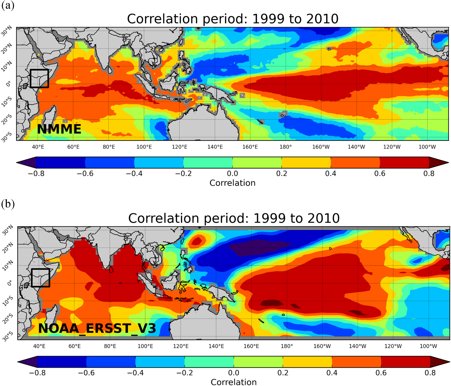
As described in section 2, the hybrid approach proposed in this study primarily harnesses the teleconnection between Indo-Pacific precipitation/SST and EA MAM precipitation. Figures 2(a) and 3(a) show the ensemble median of the spearman rank correlation between the observed EA MAM precipitation (spatially aggregated over the focus domain, within the black rectangle in the figures) and NMME MAM precipitation and SST superensemble (initialized in February) across the analog domain. Also shown is the correlation pattern between EA MAM observed precipitation and Global Precipitation Climatology Project (GPCP) precipitation dataset (Adler et al 2003), as well as NOAA's Extended Reconstructed SST version-3 (Smith et al 2008) (NOAA-ERRST-V3 SST) SST dataset in figures 2(b) and 3(b). Hence these figures demonstrate the 'observed' teleconnection. Comparison of figures 2(a) with (b) and figures 3(a) and (b) reveals that the NMME superensemble generally performs well in terms of capturing the spatial pattern and strength of the teleconnection (with absolute values of the correlation reaching ∼0.8). These also resemble the patterns described by Williams and Funk (2011) and Lyon and DeWitt (2012) linking a cool/dry Indian Ocean plus warm/wet Western Pacific plus a cool/dry central Pacific with EA rainfall declines.

Zoom In Zoom Out Reset image size

Zoom In Zoom Out Reset image size

A noteworthy observation is the negligible correlation over the EA domain itself (shown by black rectangle) (figure 2(a)). This underscores the reason why we cannot directly use the NMME superensemble MAM precipitation forecasts over the EA domain. Another noticeable difference between figures 2(a) and (b) is that NMME superensemble precipitation MAM forecasts over the Indian Ocean do not have as strong a correlation as GPCP precipitation does with EA observed MAM precipitation.

As mentioned in the section 2.2, we used the absolute value of the correlation pattern as shown in figures 2(a) and 3(a) to rescale the standardized anomalies of the NMME hindcasts over the training period. This allowed us to focus (while searching for the 'best analogs' of the target forecasts) only on those grid cells that actually have appreciable correlation with the MAM precipitation in the focus region.

Figure 4 shows a comparison between standardized anomalies of observed EA MAM precipitation and forecasts generated using the hybrid approach. Besides Indo-Pacific precipitation and SST forecasts (each used as a separate predictor) we also used the precipitation forecast over the focus region itself as a predictor. This resulted in three different sets of MAM precipitation forecasts for the focus domain. Blue box-whiskers show the ensemble spread of MAM precipitation forecasts made using Indo-Pacific precipitation as a predictor, whereas brown (faded green color) ones show the same for when Indo-Pacific SST forecasts were used as predictors (NMME superensemble MAM precipitation forecasts over the EA domain itself are referred to as regional precipitation forecasts). From this figure it can be deduced that both ensemble spread and median of MAM precipitation forecasts are much closer to the observed precipitation when Indo-Pacific precipitation or SST forecasts were used as predictors than when regional precipitation forecasts was used as predictors. Although for a number of events the observed precipitation is still beyond the ensemble spread of the MAM precipitation forecasts, the general direction of ensemble spread (i.e. below normal or above normal) aligns with the observation.

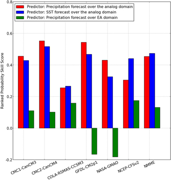
Zoom In Zoom Out Reset image size

In order to provide a quantitative evaluation of the MAM precipitation forecasts made using the hybrid approach, we calculated the RPSS of each forecast set using a climatological forecast as a 'reference forecast' (Wilks 2011). RPSS rewards a forecast for high probability values of a forecast category that is close to the actual event. An RPSS value equal to 1 indicates perfect forecast whereas values between 0 to 1 indicate that forecast is skillful and outperforms simple climatology based forecasts. The RPSS was calculated by separating the precipitation events during 1999–2010 between events below −0.44 standardized anomaly (below normal precipitation events), between −0.44 to 0.44 (near normal events) and above 0.44 (above normal events). Climatological cumulative probability (area between left tail to given Z score) of these events are 0.33, 0.67, and 1, respectively. We calculated the RPSS for the ensemble of each model separately as well as for the NMME superensemble. Figure 5 shows the RPSS values of each of the NMME models as well as the NMME superensemble for each of the three predictors. This figure shows that forecasts generated using Indo-Pacific precipitation or SST forecasts are much better than the ones made using regional precipitation as an indicator. The RPSS for the NMME superensemble was about 0.45 when Indo-Pacific precipitation or SST was used as predictor whereas it was 0.12 when regional precipitation was used as a predictor. The RPSS values for different NMME models vary between 0.25 to 0.55 when Indo-Pacific Precipitation or SST were used as predictors. Despite the variability of RPSS among the models, an RPSS of about 0.45 indicates that hybrid approach does improve the NMME superensemble based MAM precipitation forecasts for the EA region. It is worth mentioning here that the CA method inherently introduces a bias in the downscaled data. Hidalgo et al (2008) also reported a small bias in monthly climatology of downscaled precipitation and average temperature data. A quantile-quantile mapping based correction approach (e.g. Bias correction spatial downscaling method (Maurer et al 2010, Wood et al 2002)) could be used to post process the downscale data to remove the bias from the climatological mean as well as other higher moments.

Zoom In Zoom Out Reset image size

In this manuscript we demonstrate the skill of the 'hybrid approach' over 1999–2010 only. However, we also applied this method over the 1982–1998 period and found that the skill of this approach drops. As mentioned before, the skill of this hybrid approach is primarily based on the teleconnection between Indo-Pacific precipitation/SST and MAM precipitation over the EA region. We found that this teleconnection is not nearly as strong during 1982–1998 (figures S2 and S3) as it is during 1999–2010 (figures 2 and 3 and figures S3 and S4). We see weak teleconnection of EA MAM precipitation with both NMME superensemble (figures S2(a) and S3 (a)) as well as with GPCC (figure S2(b)) and NOAA ERRST V3 SSTs (figure S3(b)).

The strong teleconnection between Indo-Pacific precipitation/SST and EA MAM precipitation during the post 1999 period has been documented by other studies as well. For example, in 1999 an abrupt shift in Pacific SSTs (Lyon et al 2013) and the associated strong teleconnection between Indo-Pacific Precipitation/SST and MAM precipitation in EA (Lyon and DeWitt 2012, Hoell and Funk 2013b, 2013a). Hoell et al (2013) showed that La Nina events with cold SST over the central Pacific and warm SST over the west Pacific after 1999 resulted in an enhanced zonal SST gradient (Hoell and Funk 2013b), led to the dynamical forcing of severe drought over EA during boreal winter and spring. Although none of these studies specifically examined the dynamics responsible for this teleconnection its been hypothesized that teleconnection, post 1999 may be strong due to the combination of positive phase of Pacific Decadal Variability (Lyon et al 2013) and a warming trend in Western Pacific warm pool (Hoell and Funk 2013b, 2013a and Funk et al 2013).

As such, our choice of 1999–2010 as a training period for this analysis seems appropriate, given that our intended application is to predict hydro-climatic extremes over the next few seasons. Nevertheless, the small sample size does pose a challenge and the likelihood of the metric score being sensitive to an extreme year gets higher with a smaller sample. In order to assess the sensitivity of the skill score to a given year in the training period we performed 'leave-one-year-out' cross-validation of the 'hybrid approach' used in this study. We simply reiterated steps 1–6 described in section 2.2 after excluding a single year at a time from the training period as well the climatology used to standardize the values of forecasts and observations. We performed the cross-validation for only two models, CMC2-CanCM4 and GFDL-CM2p1, which showed the highest level of RPSS values in this analysis (figures S4 (a) and (b) respectively). We found that when extreme years such as 2000 and 2010 were excluded from the training period, the RPSS dropped. However, for years such as 2004 and 2006, the RPSS increased to about 0.7. This may be because 2000 and 2010 represent (respectively) strong canonical La Niña and El Niño years, while 2004 and 2006 were extreme dry and wet EA seasons that were likely dominated by Indian Ocean SST.

Given the small sample the variation of the RPSS to a single year is not surprising but still remains a significant improvement over when regional precipitation forecast was used as predictor.

Despite the robust nature of these results, we believe that continued decadal monitoring should accompany the application of this approach; if the current strong dichotomy between EA MAM precipitation and Indo Pacific Precipitation/SST decays the relative skill of this approach may decay rapidly. Furthermore, CO₂-driven changes to the climate are also of great importance but we do not address this topic explicitly; the influence of CO₂ on the Indo-Pacific SST/precipitation-EA relationship would be included nonetheless within these decadal and longer scale changes.

Finally, although the hybrid approach provides clear improvement over the skill of raw NMME forecasts over the EA region, the true test of the usefulness of its skill can only be done by the users of the forecast, which in our case will be the Famine Early Warning Systems Network's (FEWS NET) food analysts.

In this study we implemented and evaluated a simple 'hybrid approach' for providing seasonal forecasts of MAM precipitation in food insecure regions of EA. This approach applies the CA method to dynamical forecasts of precipitation and SST over the Indo-Pacific Ocean to provide the MAM precipitation forecasts over the focus region. Primary findings of this study are:

• (1)  
  Dynamical precipitation and SST forecasts over a large part of the Indo-Pacific ocean (specifically between latitude 30°S to 30°N and longitude 30°E to 270°E, i.e. analog domain) show high levels of absolute correlation with observed MAM precipitation over the EA (focus) region during the post 1999 period.
• (2)  
  EA MAM precipitation forecasts generated using NMME superensemble over the analog domain as predictors demonstrate much higher levels of skill (RPSS of about 0.45) than when NMME superensemble over the EA domain itself was used as predictor (RPSS of 0.12).
• (3)  
  NMME superensemble precipitation forecasts over the analog domain, when used as a predictor for forecasting EA MAM precipitation, generally provided higher levels of skill than when SST forecasts were used as predictors.

This study offers a novel tool for MAM rainfall forecasts in this region. Dynamic forecasts for the long rains exhibit very low levels of skill (Mwangi et al 2014) and the most common existing methods so far have been purely statistical and use surface or atmospheric variables (SST, sea level pressure, wind, etc) in previous months to forecast MAM rainfall (e.g. Nicholson 2014). To our knowledge this is the first study to have used dynamical seasonal forecasts based predictors for forecasting rainfall in this region. Another unique feature of this study is that it harnesses the recent teleconnection between Indo-Pacific precipitation/SSTs and EA MAM rainfall, which has led to abrupt decline in MAM rainfall in the region (Williams and Funk 2011, Lyon and DeWitt 2012), making the hybrid approach arguably more relevant than the previous methods for the current climate state. The implications of our findings could be significant for food insecure regions of EA. Skillful precipitation forecasts can improve the effectiveness of humanitarian responses (Ververs 2012) in this region by enabling aid agencies to pre-position food supplies, organize funding, and set in place appropriate contingency plans. The hybrid approach described in this study offers a definite improvement over raw NMME superensemble MAM forecasts for the EA region and is a promising tool for providing skillful precipitation forecast in this region. This approach is a computationally cheap way of harnessing the teleconnection between Indo-Pacific precipitation and SST with EA MAM precipitation. Furthermore, it provides an appropriate proof-of-concept test for potentially using regional climate models that are forced by NMME models' large-scale boundary conditions to generate precipitation forecasts in EA.

Dr Shukla is currently supported by the Postdoc Applying Climate Expertise (PACE) Fellowship Program, partially funded by the NOAA Climate Program Office and administered by the UCAR Visiting Scientist Programs. This work was also supported through USGS cooperative agreement #G09AC000001 'Monitoring and Forecasting Climate, Water and Land Use for Food Production in the Developing World', with funding from NASA SERVIR award #NNX13AQ95A for 'Leveraging CMIP5 & NASA/GMAO Coupled Modeling Capacity for SERVIR East Africa Climate Projections'; USAID Office of Food for Peace, award #AID-FFP-P-10-00002 for 'Famine Early Warning Systems Network Support'; and the USGS Land Change Science Program.