Table of contents

The recent publication of the summary for policy makers by Working Group I of the Intergovernmental Panel on Climate Change (IPCC) [1] has injected a renewed sense of urgency to address climate change. It is therefore timely to review the notion of preventing 'dangerous anthropogenic interference with the climate system' as put forward in the United Nations Framework Convention on Climate Change (UNFCCC). The article by Danny Harvey in this issue [2] offers a fresh perspective by rephrasing the concept of 'dangerous interference' as a problem of risk assessment. As Harvey points out, identification of 'dangerous interference' does not require us to know with certainty that future climate change will be dangerous—an impossible task given that our knowledge about future climate change includes uncertainty. Rather, it requires the assertion that interference would lead to a significant probability of dangerous climate change beyond some risk tolerance, and therefore would pose an unacceptable risk.

In his article [2], Harvey puts this idea into operation by presenting a back-of-the-envelope calculation to identify allowable CO₂ concentrations under uncertainty about climate sensitivity to anthropogenic forcing and the location of a temperature threshold beyond which dangerous climate change will occur. Conditional on his assumptions, Harvey delivers an interesting result. With the current atmospheric CO₂ concentration exceeding 380 ppm, a forcing contribution from other greenhouse gases adding an approximate 100–110 ppm CO₂ equivalent on top of it, and a global dimming effect of aerosols that roughly compensates for this contribution (albeit still subject to considerable uncertainty) ([1], figures SPM-1 and 2), we are on the verge of or even committed to dangerous interference with the climate system if we (1) set the risk tolerance for experiencing dangerous climate change to 1% and (2) allocate at least 5% probability to the belief that climate sensitivity is 4.5 °C or higher. In the language of the IPCC, the latter would mean that such a high climate sensitivity is anything but extremely unlikely ([1], footnote 6 and p 9), a view that is shared by many in the scientific community. Even if the risk tolerance is increased to 10%, the maximum allowable CO₂ equivalent concentration remains below 460 ppm ([2], figure 7(c)). We are bound to reach that concentration in the near future, as it can be surpassed both by addition of new greenhouse gases and by a reduction of global dimming.

Given the potential significance of this result, let us take a step back, and investigate its underlying assumptions. The concept of 'dangerous anthropogenic interference' is inextricably linked to the idea of a threshold beyond which climate change can be labeled dangerous. This idea enters Harvey's analysis in the form of a probability distribution for the—as he calls it—'harm threshold' measured in terms of global mean temperature increase since preindustrial time. It might be due to the presumption of such a threshold that climate science and society at large have had a difficult relationship with the concept of 'dangerous anthropogenic interference' (Dessai et al [3]). Nevertheless, I want to argue here, as many have done before (see Oppenheimer and Petsonk [4] for an overview), that this concept is not ill-defined. First of all, it is clear that 'dangerous interference' and the stipulation of a 'harm threshold' carry a value judgment, and therefore cannot be decided upon purely by science. This does not prevent science, however, from providing information and conceptual frameworks to facilitate such judgment (Schellnhuber et al [5]). Secondly, it is certainly true that our interference with the climate system emanates from local and national action, and that the consequences of such interference will first and foremost be felt on the local to regional scale. However, this does not need to conflict with the assessment of a global 'harm threshold'. The nexus of climate policy is inevitably global since our interference with the climate system is determined by the sum total of greenhouse gas emissions. In addition, we are living in a highly interconnected world, and it would be foolish not to take global patterns of drivers and impacts of climate change into account. Finally, some may find the assumption of a harm threshold at odds with a cost–benefit approach, since the latter implies trading off avoided climate damage with the costs of mitigation measures. However, even if such a trade-off is made, harm thresholds will occur if damage rises sharply beyond some critical amount of climate change. A look into the climate history will convince us that this is not a far-fetched idea. Climate changes in the past have often exhibited highly non-linear behaviour (see figure 1). Although the paleoclimatic record does not provide a perfect analogue to the current situation, it offers little comfort that abrupt climate change in response to our massive and rapid increase of atmospheric CO₂ concentrations might not happen in the future. Consequently, cost–benefit analyses accounting for the prospect of dangerous climate change have surfaced in recent years (e.g. Keller et al [6]). In addition, society has been prepared to set thresholds, e.g., to limit exposure to contaminants, even in situations where no clear jump in damage could be identified. And often such identification of thresholds was aided by cost–benefit analysis (e.g. Gurian et al [7]).

Is it appropriate to offer a deep time perspective on climate change such as presented in figure 1 in a discussion of 'dangerous anthropogenic interference'? Yes, because the magnitude of the anthropogenic perturbation of the carbon cycle forces us to go back far into the past, if we want to look for clues of what might happen in the future. Certainly, some of the climate changes reflected in figure 1 are a result of volcanism and continental drift, in particular the opening and closing of sea passages. However, recent data indicate that the carbon cycle was a major player in the transition from the Eocene hothouse to the modern-day icehouse world (e.g. Moran et al [11], Zachos et al [12]). The studies by Zachos et al [12] and Pearson and Palmer [13] found that carbon dioxide concentrations in the atmosphere decreased from well above 1000 ppm during the Eocene to below or around 300 ppm during the Mio-, Plio- and Pleistocene. On the basis of their data, it is likely that present-day levels of atmospheric carbon dioxide have not occurred for the last 23 million years. Moreover, projections of the growing anthropogenic perturbation of the carbon cycle in the 21st century, including scenarios that aim at stabilizing atmospheric CO₂ concentration at twice its preindustrial value, carry us to carbon dioxide levels that were last seen during the Oligocene, where major restructuring of the climate system occurred.

But what about time scales? Certainly, climate policy cannot be concerned with climate changes that unravel over millions of years. However, the slowest processes in the climate system, i.e., heat penetration into the deep ocean and changes in ice sheet volume, operate on time scales of thousands of years, with deglaciation potentially occurring much faster within hundreds of years. Hence, if the driver is sufficiently fast, rapid climate change can occur. This is evidenced in the paleoclimatic record shown in figure 1 by the event called Paleocene–Eocene Thermal Maximum (PETM) 55 million years ago. During the PETM, global temperatures rose by 5–10 °C to presumably the hottest conditions during the Cenozoic era in a matter of several thousand years (Zachos et al [14]) due to a large perturbation of the carbon cycle (Zachos et al [15]) of hitherto unknown cause (Pagani et al [16]). A millennial time scale is still far beyond the time horizon of current socio-economic activity, but this is just the time scale for the system to equilibrate (bar the removal of carbon dioxide from the atmosphere–ocean-biosphere reservoir which proceeds much more slowly [15]). Significant changes will be felt much earlier. And when it comes to assessing 'dangerous anthropogenic interference with the climate system' that has the potential to change the face of the planet for a hundred thousand or more years to come, an extension of our time horizon to several hundred years seems to be appropriate.

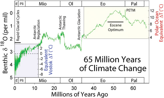
Figure 1. Any harm threshold here? Shown are δ¹⁸O stable isotope ratios (¹⁸O:¹⁶O relative to standard mean ocean water) in benthic foraminifera for the last 65 million years from Zachos et al [8]. The stable isotope ratio of the oxygen contained in the calcium carbonate of the foram shells depends on the water temperature in which they calcified (the warmer the water, the smaller δ¹⁸O). A complication arises from the fact that it also depends on the δ¹⁸O of the surrounding sea water, which is affected by latitude, evaporation and rainfall, and the presence or absence of large ice sheets. Therefore, these measurements can only be tied uniquely to past ocean temperatures for the early Cenozoic hothouse (Paleo- and Eocene) where no ice sheets existed, and for the most recent period by observing that the oxygen isotope measurements by Lisiecki and Raymo [9] are tightly correlated to temperature changes identified in the Vostok ice core (Petit et al [10]). Present day is indicated as 0. The large shifts of isotope ratio during the Oligocene also reflect changes in ice sheet volume. The figure was prepared by Robert A Rohde from published and publicly available data, and is distributed under the GNU free documentation license at www.globalwarmingart.com/wiki/Image:65_Myr_Climate_Change_Rev_png.

While the paleoclimatic record in figure 1 can inform us that 'dangerous interference with the climate system' may be in store for a species that evolved during icehouse conditions, it can not yet point us to specific harm thresholds in the climate system. Our knowledge about the climate in the past is still too sparse, and the analogy to present-day conditions too limited. In order to get a better idea about harm thresholds as the global mean temperature continues to increase, we need to turn to model projections of future climate change and associated impacts, as well as our own normative assessment of what might be labeled dangerous and what not. Given the imperfection of state-of-the-art model projections, e.g., in terms of extreme event statistics (although some have become available, see Tebaldi et al [17]), agreement on the regional scale (although improving, see [1], p 12 and figure SPM-6), and ability to model abrupt climate change, and the foreseeable disagreement between societal groups on what might be dangerous, this will certainly be an exercise in guestimating and consensus finding on some sort of uncertainty measure for the location of thresholds to dangerous climate change. In his article, Harvey offers his own take on the problem by presenting two different harm-threshold probability distributions: a stringent variant with median at 1.5 °C and 95% quantile at 2.7 °C of global mean temperature increase since preindustrial time, and a more lenient variant with median at 2.5 °C and 95% quantile at 3.8 °C. Whether or not one believes the temperature values attached to the list of impacts that Harvey offers in support of his harm assessment, there is still a value judgment about the 'dangerousness' of these impacts to be made. As Harvey points out himself, this is a question that can be informed, but not answered by science. Consequently, the allowable CO₂ concentrations to prevent dangerous anthropogenic interference with the climate system presented in Harvey's article reflect a value judgment. So it is for you, the reader, and society at large to decide whether or not these findings are significant. If your judgment about the onset of dangerous climate change lies somewhere in the range of Harvey's harm-threshold probability distributions, his results will carry meaning for you. I, for my part, can certainly answer this question in the affirmative.

Once we accept this range of harm-threshold probabilities, the natural question emerges whether Harvey's result indicating that we are on the verge of dangerous anthropogenic interference with the climate system is inevitable. Is there an easy way out by adjusting the methodological framework that would present us considerably larger allowances of carbon in the atmosphere? It does not seem so. The virtue of Harvey's back-of-the-envelope calculation is that it includes the dominant factors in a simple, but fairly robust manner, which makes it hard to significantly alter the outcome by changing the details. Harvey has considered a wide range of medians and 95% quantiles for the probability distribution of climate sensitivity, but what if we changed the shape of both the climate sensitivity and harm-threshold probability density function (PDF)? After all, there is no particular reason why they should follow a lognormal distribution as Harvey assumed. The answer to this question is harbored by equation (1) of his article. The smaller the overlap between the climate sensitivity PDF and the harm-threshold CDF, the greater the carbon allowance available without committing dangerous interference with the climate system will be. And in this respect, Harvey's assumption of lognormality for both distributions goes some way in minimizing the overlap across possible shapes for fixed median and 95% quantiles.

So what about peaking concentrations that can reach higher carbon dioxide levels because the part of the equilibrium warming they would entail will never be realized due to the time lag of the temperature response? Harvey has included this—as he calls it—climate-disequilibrium credit in his analysis, and thus his dire assessment of the proximity of dangerous interference extends to the case of transient climate change. True, he has not considered uncertainty in the heat uptake of the ocean that dominates the time lag of the temperature response along with climate sensitivity. But assuming a larger heat uptake and a slower temperature response within the confidence bounds allowed by the 20th century temperature and ocean heat content records is unlikely to change the carbon allowance by more than a few tens of ppm. Thus, Harvey's findings seem to stand firm once we underwrite the value judgment that the probability of dangerous climate change lies somewhere in the range of the harm-threshold probability distributions put forward in his article. The new sense of urgency to address climate change mirrors this judgment.

References

[1] IPCC 2007 Climate Change 2007: The Physical Science Basis - Summary for Policymakers. Contribution of Working Group I to the Fourth Assessment Report of the Intergovernmental Panel on Climate Change (Cambridge: Cambridge University Press) in preparation (available for download at http://www.ipcc.ch)

[2] Harvey L D D 2007 Allowable CO₂ concentrations under the United Nations Framework Convention on Climate Change as a function of the climate sensitivity probability distribution function Environ. Res. Lett.2 014001

[3] Dessai S, Adger W N, Hulme M, Turnpenny J, Köhler J and Warren R 2004 Defining and experiencing dangerous climate change Clim. Change64 11–25

[4] Oppenheimer M and Petsonk A 2005 Article 2 of the UNFCCC: historical origins, recent interpretations Clim. Change73 195–226

[5] Schellnhuber H J, Cramer W, Nakicenovic N, Wigley T and Yohe G (ed) 2006 Avoiding Dangerous Climate Change (Cambridge: Cambridge University Press) pp 392

[6] Keller K, Hall M, Kim S R, Bradford D F and Oppenheimer M 2005 Avoiding dangerous anthropogenic interference with the climate system Clim. Change73 227–38

[7] Gurian P L, Small M J, Lockwood J R and Schervish M J 2001 Benefit-cost estimation for alternative drinking water maximum contaminant levels Water Resources Res.37 2213–16

[8] Zachos J C, Pagani M, Sloan L, Thomas E and Billups K 2001 Trends, rhythms, and aberrations in global climate 65 Ma to present Science292 686–93

[9] Lisiecki L E and Raymo M E 2005 A Pliocene–Pleistocene stack of 57 globally distributed benthic δ¹⁸O records Paleoceanography20 PA1003

[10] Petit J R, Jouzel J, Raynaud D, Barkov N I, Barnola J M, Basile I, Bender M, Chappellaz J, Davis J, Delaygue G, Delmotte M, Kotlyakov V M, Legrand M, Lipenkov V, Lorius C, Pépin L, Ritz C, Saltzman E and Stievenard M 1999 Climate and Atmospheric History of the Past 420 000 years from the Vostok Ice Core, Antarctica Nature399 429–36

[11] Morgan K and the ACEX expedition team 2006 The Cenozic paleoenvironment of the Arctic Ocean Nature441 601–5

[12] Pagani M, Zachos J C, Freeman K H, Tipple B and Bohaty S 2005 Marked decline in atmospheric carbon dioxide concentrations during the paleogene Science309 600–3

[13] Pearson P N and Palmer M R 2000 Atmospheric carbon dioxide concentrations over the past 60 million years Nature406 695–9

[14] Zachos J C, Wara M W, Bohaty S, Delaney M L, Petrizzo M R, Brill A, Bralower, T J and Premoli-Silva I 2003 A transient rise in tropical sea surface temperature during the Paleocene–Eocene Thermal Maximum Science302 1551–4

[15] Zachos J C, Röhl U, Schellenberg S A, Sluijs A, Hodell D A, Kelly D C, Thomas E, Nicolo M, Raffi I, Lourens L J, McCarren H and Kroon D 2005 Rapid acidification of the ocean during the Paleocene–Eocene Thermal Maximum Science308 1611–5

[16] Pagani M, Caldeira K, Archer D, Zachos J C 2006 An ancient carbon mystery Science314 1556–7

[17] Tebaldi C, Hayhoe K, Arblaster J M and Meehl G A 2006 Going to the extremes: an intercomparison of model-simulated historical and future changes in extreme events Clim. Change79 185–211

Elmar Kriegler received a diploma (MS equivalent) degree in physics from the Albert-Ludwigs-University of Freiburg, Germany, in 1998, and a PhD degree in physics from the University of Potsdam, Germany, in 2005. He worked for seven years as a graduate/post-doctoral researcher at the Potsdam Institute of Climate Impact Research on topics relating to the integrated assessment of climate change. He is now a visiting researcher at Carnegie Mellon University in Pittsburgh, USA, where he works—with support by a Marie-Curie Outgoing International Fellowship from the European Union—on the evaluation of climate policies under large uncertainty about climate change.

There is a new urgency to improve the accuracy of predicting climate change impact on crop yields because the balance between food supply and demand is shifting abruptly from surplus to deficit. This reversal is being driven by a rapid rise in petroleum prices and, in response, a massive global expansion of biofuel production from maize, oilseed, and sugar crops. Soon the price of these commodities will be determined by their value as feedstock for biofuel rather than their importance as human food or livestock feed [1]. The expectation that petroleum prices will remain high and supportive government policies in several major crop producing countries are providing strong momentum for continued expansion of biofuel production capacity and the associated pressures on global food supply.

Farmers in countries that account for a majority of the world's biofuel crop production will enjoy the promise of markedly higher commodity prices and incomes^Note1. In contrast, urban and rural poor in food-importing countries will pay much higher prices for basic food staples and there will be less grain available for humanitarian aid. For example, the developing countries of Africa import about 10 MMt of maize each year; another 3–5 MMt of cereal grains are provided as humanitarian aid (figure 1). In a world where more than 800 million are already undernourished and the demand for crop commodities may soon exceed supply, alleviating hunger will no longer be solely a matter of poverty alleviation and more equitable food distribution, which has been the situation for the past thirty years. Instead, food security will also depend on accelerating the rate of gain in crop yields and food production capacity at both local and global scales.

Figure 1. Maize imports (yellow bar) and cereal donations as humanitarian aid to the developing countries of Africa, 2001–2003. MMT = million metric tons. Data source: faostat.fao.org/site/395/default.aspx.

Given this situation, the question of whether global climate change will have a net positive, negative, or negligible impact on crop yields takes on a larger significance because additional hundreds of millions of people could be at risk of hunger and the window of opportunity for mounting an effective response is closing. To answer this question, Lobell and Field use an innovative empirical/geostatistical approach to estimate the impact of increased temperature since 1980 on crop yields—a period when global mean temperature increased ∼0.4 °C [2]. For three major crops—maize, wheat, and barley—there was a significant negative response to increased temperature. For all six crops evaluated (also including rice, soybean, and sorghum), the net impact of climate trends on yield since 1980 was negative.

While the approach used by Lobell and Field can be questioned on several points^Note2, the body of their work represents an ambitious global assessment of recent climate impact on crop yields. Most noteworthy is their conclusion that: the combined effects of increased atmospheric CO₂ concentration and climate trends have largely cancelled each other over the past two decades. They contrast their finding with the conclusion of the International Panel on Climate Change (IPCC) that CO₂ benefits will exceed temperature-related yield reductions up to a 2 °C increase in mean temperature [3]. It should be noted, however, that the IPCC is coming out with a new assessment to be released in April 2007 (www.ipcc.ch/), and it remains to be seen if this conclusion still holds.

The purpose here is not to support or challenge the conclusions of either Lobell and Field or the IPCC, but rather to highlight the fact that there are substantive differences between results obtained from geostatistical assessments based on recent climate trends and actual crop yields versus assessments based on results from controlled experiments in growth chambers, greenhouses, and field enclosures and crop modeling. And while there appears to be good agreement on the predicted impact of atmospheric CO₂ enrichment on crop yields across a wide range of studies conducted using different approaches [4], there is less convincing evidence on the impact of warming temperatures.

There are three reasons for greater uncertainty about temperature effects. First, it is logistically more difficult to control temperature at elevated levels in studies that allow crops to grow in an 'open-air' environment comparable to field-grown plants. The 'free-air carbon dioxide enrichment' (FACE) systems were specifically designed to avoid such problems for study of CO₂ effects and appear to have been largely successful [4]. In contrast, growth chamber, greenhouse, and small-enclosure studies used for temperature-effect experiments have confounding effects associated with differences in humidity, air turbulence, and reduced light intensity that result from the need to more fully enclose experimental units with a transparent barrier to achieve adequate temperature control. Second, unlike CO₂ effects, yield response to temperature is often discontinuous. In many crops, pollination fails if temperatures rise above a critical threshold, which can result in dramatic yield reductions due to very small changes in temperature. Also, because climate change is predicted to increase both average temperature and temperature variability, changes in both factors must be evaluated in experiments with realistic growth conditions to fully understand climate change impact on crop yields. Such experiments would require expensive infrastructure with creative new designs—studies that have yet to be conducted, in part due to lack of adequate funding. A third factor is the interactive effect of temperature and plant nitrogen (protein) content on respiration, which is poorly understood.

In the absence of such studies, it is sobering to note that one long-term field study in which the effect of temperature on rice yield could be isolated from other factors documented a 15% decrease in yield for every 1 °C increase in mean temperature [5]. The magnitude of this decrease is considerably larger than predictions of yield decreases from higher temperature obtained from crop simulation models. Like the results of Lobell and Field [2], we see a discrepancy between estimates of the effects of warmer temperatures on crop yields based on the relationship between crop yields and temperature under field conditions versus those derived from modeling and experiments conducted under controlled conditions. As we make the historic transition from an extended period of surplus food production to one in which demand for staple crop commodities exceeds supply, there is a vital need to better understand the impact of warming temperatures on current and future crop yields.

References

[1] Council for Agricultural Science and Technology 2006 Convergence of agriculture and energy: Implications for Research and Policy CAST Commentary QTA 2006-3 (Ames, Iowa: CAST) (www.cast-science.org)

[2] Lobell D B and Field C B 2007 Global scale climate-crop yield relationships and the impacts of recent warming Environ. Res. Lett.2 014002

[3] Intergovernmental Panel on Climate Change, Working Group 2 Climate Change 2001 Impacts, Adaptation and Vulnerability IPCC Working Group 2, Third Assessment (New York: Cambridge University Press)

[4] Tubiello F N et al 2006 Crop response to elevated CO₂ and world food supply: A comment on 'Food for Thought...' by Long et al, Science 312:1918-1921, 2006 Eur. J. Agron.26 215–23

[5] Peng S, Huang J, Sheehy J E, Laza R, Visperas R M, Zhong X, Centeno G S, Khush G and Cassman K G 2004 Rice yields decline with higher night temperature from global warming Proc. Natl Acad. Sci.101 9971–5

Notes

Note1 USA (40% of global maize, 56% of global maize exports), Brazil (33% of global sugar, 36% of global sugar exports), Indonesia and Malaysia (81% of global palm oil, 88% of global palm oil exports)—2005 data from FAOSTAT: faostat.fao.org/site/395/default.aspx.

Note2 For example, the use of a 'global season' for calculating temperatures is problematic. In the case of soybean, a substantial portion of global soybean production occurs in the southern hemisphere, mostly in Brazil and Argentina, yet the global season for temperature was July–August—a time when soybean is not grown in these countries. Likewise the global season for rice was January–October, a period in which two consecutive rice crops are grown in tropical and subtropical irrigated systems of Asia—systems that account for a large portion of global rice production.

Dr Cassman is Director of the Nebraska Center for Energy Science Research at the University of Nebraska and the Heuermann Professor of Agronomy. His work focuses on ensuring local and global food security while improving environmental quality in many of the world's most productive cropping systems. Previous positions include: research agronomist in Brazil, Egypt and the Philippines; faculty member at the University of California-Davis; division/department head at the International Rice Research Institute and the University of Nebraska. He received a PhD from the University of Hawaii's College of Tropical Agriculture (1979) and a BS in Biology from the University of California, San Diego (1975).

Article 2 of the United Nations Framework Convention on Climate Change (UNFCCC) calls for stabilization of greenhouse gas (GHG) concentrations at levels that prevent dangerous anthropogenic interference (DAI) in the climate system. Until recently, the consensus viewpoint was that the climate sensitivity (the global mean equilibrium warming for a doubling of atmospheric CO₂ concentration) was 'likely' to fall between 1.5 and 4.5 K. However, a number of recent studies have generated probability distribution functions (pdfs) for climate sensitivity with the 95th percentile of the expected climate sensitivity as large as 10 K, while some studies suggest that the climate sensitivity is likely to fall in the lower half of the long-standing 1.5–4.5 K range. This paper examines the allowable CO₂ concentration as a function of the 95th percentile of the climate sensitivity pdf (ranging from 2 to 8 K) and for the following additional assumptions: (i) the 50th percentile for the pdf of the minimum sustained global mean warming that causes unacceptable harm equal to 1.5 or 2.5 K; and (ii) 1%, 5% or 10% allowable risks of unacceptable harm. For a 1% risk tolerance and the more stringent harm-threshold pdf, the allowable CO₂ concentration ranges from 323 to 268 ppmv as the 95th percentile of the climate sensitivity pdf increases from 2 to 8 K, while for a 10% risk tolerance and the less stringent harm-threshold pdf, the allowable CO₂ concentration ranges from 531 to 305 ppmv. In both cases it is assumed that non-CO₂ GHG radiative forcing can be reduced to half of its present value, otherwise; the allowable CO₂ concentration is even smaller. Accounting for the fact that the CO₂ concentration will gradually fall if emissions are reduced to zero, and that peak realized warming will then be less than the peak equilibrium warming (related to peak radiative forcing) allows the CO₂ concentration to peak at 10–40 ppmv higher than the limiting values given above for a climate sensitivity 95th percentile at 4.5 K. Even allowing for the difference between peak realized and peak equilibrium warming, and assuming that present non-CO₂ GHG forcing can be cut in half, a CO₂ concentration of 410 ppmv or less constitutes DAI for every combination of harm-threshold pdf and risk tolerance considered here if the 95th percentile of the climate sensitivity pdf is 4.5 K or greater.

Changes in the global production of major crops are important drivers of food prices, food security and land use decisions. Average global yields for these commodities are determined by the performance of crops in millions of fields distributed across a range of management, soil and climate regimes. Despite the complexity of global food supply, here we show that simple measures of growing season temperatures and precipitation—spatial averages based on the locations of each crop—explain ∼30% or more of year-to-year variations in global average yields for the world's six most widely grown crops. For wheat, maize and barley, there is a clearly negative response of global yields to increased temperatures. Based on these sensitivities and observed climate trends, we estimate that warming since 1981 has resulted in annual combined losses of these three crops representing roughly 40 Mt or $5 billion per year, as of 2002. While these impacts are small relative to the technological yield gains over the same period, the results demonstrate already occurring negative impacts of climate trends on crop yields at the global scale.

An increasingly diverse set of hybrid-electric vehicles (HEVs) is now available in North America. The recent generation of HEVs have higher fuel consumption, are heavier, and are significantly more powerful than the first generation of HEVs. We compare HEVs for sale in the United States in 2007 to equivalent conventional vehicles and determine how vehicle weight and system power affects fuel consumption within each vehicle set. We find that heavier and more powerful hybrid-electric vehicles are eroding the fuel consumption benefit of this technology. Nonetheless, the weight penalty for fuel consumption in HEVs is significantly lower than in equivalent conventional internal combustion engine vehicles (ICEVs). A 100 kg change in vehicle weight increases fuel consumption by 0.7 l/100 km in ICEVs compared with 0.4 l/100 km in HEVs. When the HEVs are compared with their ICEV counterparts in an equivalence model that differentiates between cars and sports-utility vehicles, the average fuel consumption benefit was 2.7 l/100 km. This analysis further reveals that a HEV which is 100 kg heavier than an identical ICEV would have a fuel consumption penalty of 0.15 l/100 km. Likewise, an increase in the HEV's power by 10 kW results in a fuel consumption penalty of 0.27 l/100 km.