


Abstract
The recent detection of Earth-sized planets in the habitable zone of Proxima Centauri, Trappist-1, and many other nearby M-type stars has led to speculations whether liquid water and life actually exist on these planets. To a large extent, the answer depends on their yet unknown atmospheres, which may, however, be within observational reach in the near future by JWST, ELT, and other planned telescopes. We consider the habitability of planets of M-type stars in the context of their atmospheric properties, heat transport, and irradiation. Instead of the traditional definition of the habitable zone, we define the biohabitable zone, where liquid water and complex organic molecules can survive on at least part of the planetary surface. The atmospheric impact on the temperature is quantified in terms of the heating factor (a combination of greenhouse heating, stellar irradiation, albedo, etc.) and heat redistribution (horizontal energy transport). We investigate the biohabitable domain (where planets can support surface liquid water and organics) in terms of these two factors. Our results suggest that planets orbiting M-type stars may have life-supporting temperatures, at least on part of their surface, for a wide range of atmospheric properties. We apply this analyses to Proxima Cen b and the Trappist-1 system. Finally, we discuss the implications for the search of biosignatures and demonstrate how they may be used to estimate the abundance of photosynthesis and biotic planets.
Export citation and abstract BibTeX RIS
1. Introduction
Recent data of the Kepler mission show that 10%–50% of M dwarfs have small planets orbiting within their habitable zone (HZ; Batalha et al. 2013; Dressing & Charbonneau 2015), which implies that such planets could be found within less than 10 light years from Earth (Wandel 2015, 2017a). A high abundance of Earth-size volatile-rich planets close to low-mass M-stars is also supported by theoretical arguments and planetary formation models (Alibert & Benz 2017). Transiting planets of M-type stars are also easier targets for the detection of biosignatures (Seager & Deming 2010). The detection of an Earth-sized planet within the HZ of Proxima Centauri (Anglada-Escudé et al. 2016) and the Trappist-1 system (Gillon et al. 2017) has driven much interest in the question of whether planets orbiting red dwarf stars could support life, despite such planets being gravitationally locked with eternal day and eternal night hemispheres (Heller et al. 2011; Leconte et al. 2015). Other threats to life come from the enhanced EUV radiation and X-ray flares of the host star (e.g., Ribas et al. 2016), atmospheric erosion (Zendejas et al. 2010), runaway greenhouse, and water loss (Kopparapu 2013; Luger & Barnes 2015). Over the last decade, many authors have suggested that these factors would be less severe than previously thought (Scalo et al. 2007; Tarter et al. 2007; Seager & Deming 2010; Gale & Wandel 2017). Although planets in the HZ of M-type stars are irradiated by much higher EUV and X-ray fluxes than Earth, many evolutionary models of M dwarfs lead to water-rich planets. Furthermore, a prime atmosphere that is massive enough could survive the extended erosion during the energetic early evolution of M dwarfs (e.g., Tian 2009), while recent simulations show that even terrestrial atmospheres could survive for billions of years on some habitable planes orbiting M dwarfs, e.g., in the case of Trappist-1 (Dong et al. 2018).
A major condition for the evolution of life is the capability to support liquid water and surface temperatures in the range adequate for complex organic molecules. This condition depends not only on the irradiation from the host stat, but to a large extent on the effect of the planet's atmosphere. Global climate models (GCMs) using radiative transfer, turbulence, convection, and volatile phase changes can calculate the conditions on planets, depending on the properties of their atmospheres. Such 3D climate models of M-dwarf planets show the presence of liquid water for a variety of atmospheric conditions (e.g., Pierrehumbert 2011a; Wordsworth 2015). Climate modeling studies have shown that an atmosphere only 10% of the mass of Earth's atmosphere can transport heat from the day side to the night side of tidally locked planets, enough to prevent atmospheric collapse by condensation (Joshi et al. 1997; Scalo et al. 2007; Tarter et al. 2007; Heng & Kopparla 2012). On locked planets, the water may be trapped on the night side (e.g., Leconte et al. 2013), but on planets with enough water or geothermal heat, part of the water remains liquid (Yang et al. 2014). Three-dimensional GCM simulations of planets in the HZ of M dwarfs support scenarios with surface water and moderate temperatures (Yang et al. 2014; Leconte et al. 2015; Owen & Mohanty 2016; Turbet et al. 2016; Kopparapu et al. 2016; Wolf 2017 to name a few). A variety of surface temperature distributions emerges. Although rocky planets with no or little atmosphere, like Mercury, have an extremely high day–night contrast and planets with a thick, Venus-like atmosphere tend to be nearly Isothermal, intermediate cases, with up to 10 bar atmospheres conserve significant surface temperature gradients (e.g., Selsis et al. 2011). Wolf et al. (2017) find (for F-K type hosts) that stable habitable ocean worlds can be maintained for global mean surface temperatures in the range of 235–355 K.
It is instructive to consider whether similar results can be obtained more generally, using basic principles. Lower-order climate models for synchronously rotating planets have been discussed by several authors (Haberle et al. 1996; Pierrehumbert 2011a; Heng & Kopparla 2012; Mills & Abbot 2013; Wordsworth 2015; Koll & Abbot 2016).
Rather than the usual treatment of the HZ, defined as the region around a star where planets can support liquid water (e.g., Kasting et al. 1993), we investigate the biohabitable zone, where surface temperatures can support, in addition to liquid water, complex organic molecules also.1
As the properties that affect the atmosphere and surface temperature distribution are complex, entangled, and difficult for observational determination and delineation, we combine them in merely two factors: redistribution and atmospheric heating. In this two-dimensional parameter space, we chart the domain where liquid water and life-supporting temperatures are present on at least part of the planet's surface.
In Section 2, we derive a simple model for the surface temperature distribution of tidally locked planets in terms of the radiative and atmospheric heating and the horizontal heat transport. In Section 3, we define the heating factor of the planet's atmosphere. Section 4 demonstrates the model parameters for the terrestrial planets in the solar system, and Section 5 applies the model to the Trappist-1 planets. In Sections 6 and 7, we define the biohabitable zone and investigate its dependence on the atmospheric properties in terms of the heating factor and the heat transport. Finally, in Sections 8 and 9, we consider the implications for biosignature detection and estimate the abundance of biotic planets.
2. Thermal Models for Tidally Locked Planets
Planets within the HZ of M dwarfs are often close enough to their hosts to be tidally locked. In synchronously orbiting planets, horizontal energy transport has a major impact on the surface temperature, as it determines the horizontal temperature gradient and the temperature on the night hemisphere. Overall, the surface temperature is determined by three major factors: irradiation from the host star (insolation), atmosphere (transmission and greenhouse effect), and horizontal heat transport. Energy redistribution due to convection can in principle be determined from the atmospheric properties (atmospheric pressure, heat capacity and wind speed, global circulation patterns), which may be identified with broadband thermal phase curves; see, e.g., Wang et al. (2014). However, these data may be difficult to obtain and disentangle in exoplanets. Hence, we describe the heat redistribution in a parametric form, with a global redistribution parameter (f) and a local one (b). We subsequently show that these two parameters are related.
Following previous works (Haberle et al. 1996; Goldblatt 2016), we separate the energy balance into day and night hemispheres, with advective interchange of energy.
Atmospheric temperatures of aquatic locked planets may be nearly uniform horizontally, as approximated by the Weak Temperature Gradient model (Joshi et al. 1997; Merlis & Schneider 2010), while dry, low surface pressure, tidally locked planets may have larger horizontal temperature differences, in particular between the day and night sides (Koll & Abbot 2016). Intermediate cases can be described by a global energy redistribution scheme (e.g., Pierrehumbert 2011a). In addition to global redistribution, we consider local heat transport, representing small-scale advection and turbulence in the atmospheric surface layer, which has been demonstrated by 3D models to be essential for the global energy balance on tidally locked planets (Wordsworth 2015).
2.1. Tidally Locked Planets with Global Redistribution
Without an atmosphere, the surface temperature of a slowly rotating planet is determined only by the irradiation from the host star and the latitude, that is, the angular distance θ from the substellar point,

Here, σ is the Stefan Boltzman constant, A is the Bond albedo, and F = cos(θ). The irradiation or insolation is given by S = L*/4πa2, where a is the distance of the planet from its host star and L* is the host star's luminosity.2
Planets with an efficient horizontal heat spread or rapidly rotating ones are nearly isothermal, the equilibrium surface temperature being

The atmosphere has two main effects on the surface temperature: vertical energy exchange between the atmosphere and the surface, and horizontal heat transport. The former can be described by an energy balance equation of the form (e.g., Mills & Abbot 2013)

where Ta is the atmospheric temperature, ea is the atmospheric long-wave emissivity, and ca is the surface-to-atmosphere exchange constant. In the following, we replace the two unknown parameters ea and ca by a single one (the heating factor H; Section 2.2), in which we include also the insolation and the albedo. We reduce the extra variable Ta by assuming the atmosphere is horizontally isothermal (the Weak Temperature Gradient model, which has been shown to be a very good approximation in slowly rotating planets; Pierrehumbert 2011a, 2011b), and by implicitly replacing the last term on the right-hand side (rhs) with the horizontal redistribution mechanism.3
Horizontal energy redistribution transports heat across the temperature gradient created by latitude-dependent irradiation. We describe this effect by assuming that at every latitude of the day side, a fixed fraction f of the heat due to the radiation from the host star is removed and homogeneously distributed over the entire planet,
where θ is the latitude, measured from the substellar point (there, θ = 0, while θ = 90° is the terminator, separating the day and night hemispheres). The global redistribution parameter may be in the range 0 ≤ f ≤ 1 and is primarily determined by the atmospheric pressure and circulation. Three-dimensional climate models show that f is influenced also by the planet's rotation, size, and surface friction (e.g., Carone et al. 2015).
Geothermal heating of the order of that of Earth, 0.1 W m−2 (Davies & Davies 2010), may be ignored, as it is less than 10−3 of Earth's irradiation. However, for planets in the inner HZ of M-type stars, tidal heating may be important (Dobbs et al. 2017). This issue will be considered in a subsequent work.
Solutions of Equation 1(a) are shown in Figure 1. We have used the insolation of Proxima Centauri b (Anglada-Escudé et al. 2016), S = 0.65S⊕, where S⊕ = 1362 Watt m−2 is the solar constant at Earth's orbit. We have assumed an albedo of A = 0.1 (like the Moon). Cloud (or ice) coverage (e.g., Yang et al. 2014) would raise the albedo, lowering the temperature. For example, if A = 0.3 (like Earth), the curves in Figure 1 need to be multiplied by 0.94.

Figure 1. Surface temperature distribution for various global heat redistribution rates, with the insolation of Proxima Cen b. Equilibrium temperature is plotted vs. latitude for different values of the global redistribution factor f. When f = 1 (full global redistribution), the planet becomes isothermal. A small amount of local heat redistribution has been assumed in order to avoid unrealistically sharp temperature changes.
Download figure:
Standard image High-resolution image2.2. The Atmospheric Impact
The atmosphere can have a major impact on the surface temperature. We follow the analyses of Guillot (2010), adapting it to rocky planets. Part of the stellar irradiation is absorbed and scattered by the atmosphere, which may be described by the parameter α, defined as the fraction of short-waveband irradiation at the top of the atmosphere reaching the surface.
Strictly speaking, α = exp[−τSW/cos(θ)], where τSW is the vertical optical depth of the atmosphere in the short waveband. However, assuming the atmosphere is relatively transparent in the short waveband, this expression may be simplified by taking a weighted average over latitude. The values of α for the terrestrial planets of the solar system are given in Table 1.
Table 1. Data and Calculated Atmospheric Parameters for the Terrestrial Planets of the Solar System
| Earth | Venus | Mars | Mercury | |
|---|---|---|---|---|

|
1 | 0.723 | 1.52 | 0.387 |
 (K) (K) |
278 | 327 | 225 | 447 |
 (K) (K) |
288 | 737 | 210 | 100–700 |

|
0.28 | 0.9 | 0.25 | 0.068 |

|
0.48 | 0.1 | 1 | 1 |

|
2.3 | 2500 | 0.003 | 0 |

|
6 | 50 | 0.3 | 0 |

|
0.95 | 1 | 0.85 | 0.003 |

|
1.15 | 50 | 0.33 | 6.2 |

|
1.15 | 26 | 0.75 | 0.93 |
Note. Teq is the equilibrium surface temperature without an atmosphere, T is the measured surface temperature, and A is the Bond albedo. The greenhouse heating Hg or the long-wave optical depth τLW are derived from the measured albedo and transmissivity. Then, the heating factors are given by Hatm = (T/Teq)4 and H = Hatm/a2.
Download table as: ASCIITypeset image
The atmospheric attenuation of the planet's radiative cooling, mainly in the infrared, is determined by the abundance (partial pressure) of greenhouse gases, such as CO2, CH4, N2O, and H2O. We define the greenhouse heating parameter Hg as the amount of increase in the thermal energy at the surface due to the greenhouse effect. It can be shown (e.g., Guillot 2010) that the greenhouse heating is related to the optical depth,

where τLW is the optical depth of the atmosphere in the long wavelength regime. A planet with no atmosphere, or with no greenhouse gases, has Hg = 1. For an optically thick atmosphere, f ≈ 1, and the planet becomes nearly isothermal, with

and Teq is the equilibrium isothermal surface temperature (Equation 1(b)). This result resembles the scaling relation derived by Pierrehumbert (2011b) for the surface temperature of an isothermal planet with an optically thick atmosphere.4 The lowest temperature on the night side (at the point opposite to the substellar one, θ = 180°), from Equations 1(b) and (c), is given by

Since in the long-waveband radiation is scattered in all directions, the greenhouse effect redistributes heat not only vertically but also horizontally. For an optically thin atmosphere, τLW < 1, αHg ∼ 1, and the effective redistribution is approximately f ∼ τLW, hence Equation 2(b) gives

A similar lower limit, Tmin = Teq(τLW/2)1/4, has been found by Wordsworth (2015) for the night-side temperature of locked planets with optically thin atmospheres.
2.3. Local Heat Redistribution
In addition to governing global heat redistribution, atmospheric advection can transport heat locally by small-scale advection. Altogether we add to Equation 1(a) a term of local heat transport (LHT) denoted by  , in addition to the factors of atmospheric screening (α) and greenhouse heating (Hg) discussed above, giving

LHT transports energy in the direction perpendicular to the temperature gradient, hence the heat flux at a given latitude is proportional to the negative derivative of the temperature. The overall energy flow is proportional to  , or
, or  , where x is the horizontal coordinate, R is the planet's radius, and the sine term gives the dependence of the surface area element on the latitude. The net heating is the derivative of the energy flow,
where B is the advection parameter (cf., Haberle et al. 1996; Goldblatt 2016),

Here, ps is the surface atmospheric pressure, cp is the heat capacity (e.g., for air cp = 1 kJ Kg−1 K−1), u is the wind speed, and g is the surface gravity. For example, on Earth at sea level, B = 15 (u/10 m s−1) Wm−2 K−1.
Substituting these expressions for  , Equation (3) gives

Solving Equation (5) for the temperature at θ = 0 (the substellar point, using Equation 1(c)) gives
while at the opposite point (Equation 2(b))

2.4. The Dimensionless Energy Balance Equation
Equation (5) can be written in a dimensionless form. Defining a normalized temperature y = T/T0 and dividing by  give
give

where the dimensionless local heat transport parameter b is given by

Equation (7) can be solved numerically (Figures 2, 3) with the boundary condition y(0) = 1, y'(0) = 0. Physically, b is the advection parameter multiplied by the ratio of temperature to radiative heating at the substellar point. This choice of normalization is supported by 3D simulations which suggest that the local advection increases with radiative heating (Wordsworth 2015). As an example, the Earth atmosphere at sea level has b ≈ 6. Typical values of b for the terrestrial planets of the solar system are listed in Table 1.
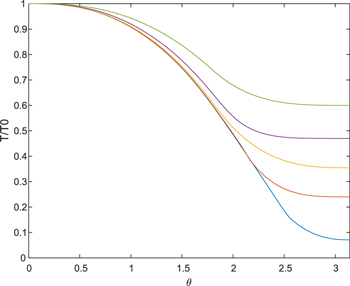
Figure 2. Normalized temperature profiles for different values of the global redistribution parameter (marked on the right axis, f = 10−4, 0.01, 0.05, 0.2, 0.5) with moderate LHT (b = 0.5). For large global redistribution (f > 0.3), the normalization factor T0 depends on f.
Download figure:
Standard image High-resolution image
Figure 3. Normalized temperature profiles for several values of the local transport coefficient (b = 0.1, 0.5, 1, 2, 5, 10, and 20; some are marked on the right axis), with f = 0. The dashed–dotted curve corresponds to Equation 1(a) with zero redistribution. Note that for b > 1, the normalization factor T0 depends on b.
Download figure:
Standard image High-resolution imageUnlike5 f, b is not a free parameter, as the local advective heat transport is determined by the planetary and atmospheric properties (Equation (4)). To some extent, global and local heat redistribution are related; when the LHT is not small (b > 1), heat is globally redistributed (cf., Figure 3), hence large LHT may be approximated by increasing the global heat redistribution parameter. The two processes are complementary, as global redistribution may have sources other than advection, while LHT smoothens temperature gradients on smaller scales. Although in some cases the two parameters, f and b, can be combined, for the sake of generality we retain both heat redistribution terms in Equations (5) and (7).
When b ≪ 1 (LHT is small compared to radiative heating),  can be ignored and Equation (3) can be solved analytically,

where a is the semimajor axis of the planet's orbit expressed in astronomical units and L is the host's luminosity. For a nearly circular orbit, the insolation relative to Earth is given by  . Equations 2(a) and 9 give
where H is defined by Equation (12). At the substellar point (θ = 0°), Equation (9) coincides with Equation 6(a). When the LHT is small (b < 1), its impact on the global energy balance is small, and the night side is nearly isothermal. This can be seen in Figures 1 and 2. Far from the terminator, the night-side temperature approaches T = (f/4)1/4T0, hence y(180°) = (f/4)1/4. Similar results are obtained by GCM calculations (e.g., Wordsworth 2015; Koll & Abbot 2016).
Numerical solutions of Equation (7) are shown in Figures 2 and 3. Note that in general, T0 depends on f (Equation 6(a)). While for f < 0.3 this dependence is negligible, for larger values of f, global heat redistribution can significantly reduce the substellar temperature.
Figure 3 shows that when the LHT is comparable to or larger than the radiative heating from the host star (b > 1), its impact on the energy balance cannot be ignored, as it transports significant amounts of energy from the day hemisphere to the night one. Energy conservation implies

When b ≪ 1, T0 is given by Equation 6(a), and Equation (10) is satisfied. In general, Equation (10) gives
where

and H is the heating factor (Equation (12)).
For large LHT (b ≫ 1), the planet becomes nearly isothermal (y = 1), as in the case of f = 1 (Equation 2(a)). Also in this case, it is easy to see that Equations (10) and (11) are satisfied, and we may replace b with an effective global heat redistribution f, as discussed after Equation (8).
3. The Heating Factor
The albedo and atmospheric transmissivity can be combined to give an effective reflectivity (1 – A)α. In Equations (8) and (9), this term appears together with the greenhouse factor and the insolation. Hence, it is convenient to combine the albedo, the atmospheric screening and heating effects, and the insolation into a single dimensionless parameter (already used above), which we call the heating factor,

Here, s = S/S⊕ is the insolation relative to Earth, and Hg is the greenhouse factor. Figure 4 shows the surface temperature profiles for various values of the heating factor.

Figure 4. Temperature profiles for several values of the heating factor (from below, H = 0.1, 0.3, 1, 3, 10). A global heat transport of f = 0.2 and a moderate (b = 0.5) LHT are assumed. The liquid water temperature range at 1 bar is indicated by the shaded blue area.
Download figure:
Standard image High-resolution imageAs the planet's insolation is usually known, it is useful to leave it out of the total heating, and define the atmospheric heating factor, which describes only the atmospheric impact (and the albedo),

Figure 4, as well as Figures 6–7 below, can be modified to use the atmospheric heating factor rather than H, scaling the temperatures by s1/4, namely T(Hatm) = s−1/4T(H). For example, for Proxima Cen b, this factor is (0.65)−1/4 = 1.1. This adjustment is applied to the Trappist-1 planets in Figure 6.
Atmospheric heating can have a strong influence on the existence of liquid water, but other processes may also play a role. Under certain conditions, water on tidally locked planets may be transported from the day side and deposited by precipitation at the night side, where it is trapped as ice (Leconte et al. 2013; Menou 2013; Yang et al. 2014). However, as noted by these authors, complete trapping will occur only for planets with low water content and geothermal heat flux lower than that of Earth.
4. The Solar System
We demonstrate some values of the heating factors and the other parameters defined above for different atmospheres and insolations by calculating them for the terrestrial planets of the solar system, for which the albedo and atmospheric data are well-known (Table 1). The atmospheric heating factor can be determined by comparing the effective surface temperature to the equilibrium temperature (the planet's surface temperature calculated without the atmospheric effects) and A = 0, that is, Hatm = 1. For L = L⊙, the equilibrium temperature is given by Teq = 278a−2 K, where a is the average distance from the Sun in astronomical units.
Some indicative values of the albedo for common planetary surfaces are A = 0.15 (bare rock), 0.3 (patch water clouds, as in present Earth), and 0.6 (complete water cloud coverage). The greenhouse factor is calculated using the relation
where the atmospheric heating factor is given by Hatm = (T/Teq)4. For example, Earth's atmosphere (0.78 bar N2, 0.21 O2, and 375 ppm CO2) has Hatm = 1.15, and its short-wave transmissivity is α = 0.48, hence Hg = 3.3 and τLW = 2.3.
The larger the partial atmospheric pressure and the abundance of greenhouse gases, the stronger is the greenhouse effect. For example, for Venus we get αHg = 250. In order to estimate the greenhouse factor of the Venusian atmosphere (∼90 bar CO2), we assume α = 0.1. For the airless Mercury, we assume α = Hg = 1, and f may be determined from Equation 15(a) below.
The relatively fast rotating terrestrial planets (Earth and Mars) are nearly isothermal, so they may be considered to have an effective global redistribution parameter near unity (actually slightly less, because of the day–night differences). Also, Venus is nearly isothermal, despite its synchronous rotation, because of its dense atmosphere and cloud cover, which efficiently smoothen surface temperature gradients. For Mercury, an effective global redistribution parameter is estimated from the lowest surface temperature on the night side and Equation 2(b). The parameter b is calculated from Equation (8), with u assumed to be 5 m s−1 for Earth, 20 m s−1 for Mars, and 1 m s−1 for Venus.
For exoplanets, the amount of heat redistribution and the albedo may be estimated by observing the thermal phase variation, which could be measured by JWST (Kreidberg & Loeb 2016). The albedo may also be determined by high-contrast spectroscopy, which can be accomplished by just one night of the planned ELT (Snellen et al. 2015).
Figure 5 shows the four terrestrial planets of the solar system in the T versus H diagram. Note that Venus, Earth, and Mars have average temperatures consistent with the equilibrium (isothermal surface) green curve, while Mercury's temperature gradient is larger than that of a locked planet with a global redistribution parameter of f = 0.1 (the dashed curves), consistent with the effective value of f calculated above.

Figure 5. Locations of the four terrestrial planets of the solar system in the T vs. H diagram. The green solid curve shows the equilibrium temperature for an isothermal planet, while the dashed curves show the highest and lowest surface temperatures of a tidally locked planet with 10% global redistribution (f = 0.1).
Download figure:
Standard image High-resolution image5. The Trappist-1 System
We demonstrate the derivation of the parameter values for extra solar planets with a given irradiation but an unknown atmosphere, by calculating the biohabitable range6 for the Trappist-1 planets, in terms of the heating factor. The insolations of the Trappist-1 planets can be determined from their measured periods (determining the distances from the host star). The insolation is calculated using the bolometric luminosity. As a caveat, note that if the τLW of the planet's atmosphere is not small, only a fraction of the irradiative flux penetrates the atmosphere and reaches the surface, as most of the luminosity in Trappist-1 host is in the long-waveband range. The habitability and climate calculation of the Trappist-1 planets have been attempted by several authors using GCM-codes. For global ocean planets, Wolf (2017) concludes that only Trappist-1e is likely to be habitable. However, our model also takes into account local habitability on semi-dry planets, e.g., in water-belt worlds.
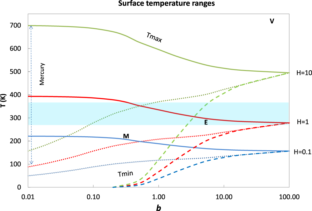
Figure 6 shows the surface temperature distribution for each of the six inner planets of the Trappist-1 system, assuming a 10% global heat redistribution (f = 0.1) and an atmospheric heating factor Hatm = 1, similar to that of Earth's atmosphere. We note that the five inner planets could support liquid water and organic molecules on some part of their surface. Trappist-1g could be marginal, being almost entirely frozen, with an eyeball configuration of liquid water at the substellar point. With an atmosphere of a heating factor four times lower than that of Earth (Hatm = 0.3; shown in Figure 6 by the lower dashed curve for Trappist-1g), all planets except f and g could support a biohabitable region. For an atmospheric heating factor ∼3 times larger than that of Earth (Hatm = 3; upper dashed curve for Trappist-1b) without moist greenhouse runaway, the five outer planets could support a biohabitable region, with Trappist-1b being marginal, having a night-side temperature of nearly 373K.
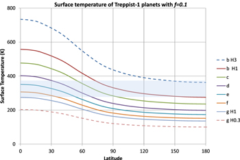
Figure 6. Surface temperature profiles for the six inner Trappist-1 planets. The global heat transport parameter is taken as f = 0.1 and the LHT parameter as b = 0.5. The continuous curves denote an atmospheric heating factor of Hatm = 1. Dashed curves mark the coldest (g) and hottest (b) planets with Hatm = 0.3 and Hatm = 3, respectively. The temperature range of liquid water at 1 bar is indicated by the shaded blue area.
Download figure:
Standard image High-resolution imageAn increased Hatm may be due to a larger greenhouse factor (i.e., larger τLW). As noted above, scattering of the incoming long-waveband radiation from the host may reduce the amount of stellar radiation actually arriving at the planet surface, lowering the atmospheric screening parameter α and producing a negative feedback on the heating factor. For example, if the atmospheric scattering in the long waveband reduces the effective heating factor a by a factor of 3, we may see from Figure 6 that atmospheres with Hatm as high as ∼10 could support biohabitable conditions for the six inner Trappist-1 planets.
6. The Biohabitable Zone
The traditional habitable zone is associated with the existence of liquid water on the planetary surface. The extent of the liquid water zone around the host star may be described by the Kombayashi–Ingersoll radiation limit (Kombayashi 1967; Ingersoll 1969; Kasting et al. 1993), also called the "runaway greenhouse" limit. The inner edge of the habitable zone is located at the distance from the host star, where surface water is completely vaporized or at which water reaches the upper atmosphere, where it can be dissociated by ultraviolet radiation (unless, as in Earth's atmosphere, there is cold-trapping of water at a tropopause-like layer). Runaway greenhouse processes may push this inner edge outwards, while cloud coverage may push it inwards to radii as small as about 0.5 au for a Sun-like host (e.g., Kasting et al. 1993; Yang et al. 2016). The outer edge of the HZ is determined by water being completely frozen on the planet surface. For planets with a present Earth atmosphere and Sun-like host, this limit may be not much larger than Earth's orbit, because of the positive feedback of the runaway snowball effect. The outer limit may, however, be increased considerably, beyond 2 au for a Sun-like host, by increasing the CO2 atmospheric abundance, e.g., by outgassing and geological CO2 enrichment of the atmosphere (Froget 2013). The freezing point of water may also be lowered by high salinity.
In the following, we will define the HZ not in the spatial sense, but rather in the climatic sense, quantified in the parameter space spanned by the heating factor and heat redistribution. Wolf et al. (2017) find four stable climate states defined by their global mean surface temperatures (Ts): snowball (Ts < 235 K), water belt (235 K < Ts < 250 K), temperate (275 K < Ts < 315 K), and moist greenhouse (Ts > 330 K), with the latter three able to maintain habitable ocean worlds. It has been claimed that the outer boundary of the HZ may be reduced by snowball limit cycles, but Haqq-Misra et al. (2016) find that those cannot occur on K- or M-star planets.
We define the "Biohabitable zone," which differs from the usual HZ in two ways. First, rather than quantifying the spatial boundaries where planets can globally support liquid water, we consider the domain in the parameter space, defined by atmospheric heating and heat redistribution, where liquid water and life-supporting temperatures occur at least on part of the surface of a tidally locked planet.
Depending on the pressure, water may be liquid at temperatures far beyond the temperatures allowing organic complex molecules, and the Kombayashi–Ingersoll limit may not be relevant for biohabitability, in particular if oxygenic photosynthesis is considered (cf., Gale & Wandel 2017). We adopt 373 K as a conservative upper temperature. On the one hand, this value may be on the low side, as organic molecules and even life may survive at somewhat higher temperatures, as demonstrated, e.g., by extremophile life forms found near thermal vents in the bottom of Earth's oceans. On the other hand, moist greenhouse runaway may start at average global surface temperatures as low as 355 K (Wolf et al. 2017). In any case, our results are not very sensitive to minor variations of the temperature range.
The lower temperature limit is naturally chosen as the freezing point of water, which is only weakly dependent on pressure, and is widely accepted as a lower limit for organic processes. Of course, this limit is also somewhat conservative, as high salinity can lower the freezing point. Still, lower surface temperatures do not exclude liquid water and life under an ice cover, e.g., in the case of geothermal or tidal heat like in Europa and Enceladus. As mentioned above, tidal heating may be important in habitable planets of M-type stars (Dobbs et al. 2017).
On synchronously orbiting planets, the highest surface temperature, T0, occurs at the substellar point, θ = 0. When b < 1, T0 is given by Equation 6(a). If b > 1, it needs to be modified using Equation (11). The lowest surface temperature occurs at the far end of the night hemisphere, the opposite side of the substellar point, θ = 180°. When b < 1, it is given by (Equations 6(a) and (b))

When b > 1, LHT cannot be ignored and Tmin must be calculated numerically. However, also for moderate values of f and b, Equation (14) turns out to be a good approximation. Combining Equations 6(a), 6(b), (12), and (14), the lowest and highest temperatures can be written as

The corresponding values of the dimensionless temperature are ymax = 1 and

When the LHT is large (b > 10), it dominates global heat redistribution (cf., Wordsworth 2015). In that case, the planet is nearly isothermal: y ∼ 1 and

Figures 7 and 8 show the highest and lowest surface temperatures as a function of the heat redistribution parameters f and b, respectively, for a few values of the heating factor H. The f and b values of the terrestrial planets of the solar system are taken from Table 1.

Figure 7. Highest and lowest surface temperatures Tmin (dashed) and Tmax (solid), vs. the global redistribution parameter, f (with b = 0), for three values of the heating factor H, marked on the right axis. The liquid water range for 1 bar is shown by the shaded blue area. Letters indicate the terrestrial planets of the solar system.
Download figure:
Standard image High-resolution image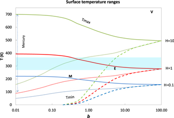
Figure 8. Surface temperatures Tmin (dashed) and Tmax (solid), vs. the local transport parameter, b, for three values of the heating factor H, marked on the right axis. The dotted curves represent a more realistic approximation, allowing for a modest global redistribution when local heat transport is low (see text). The liquid water range for 1 bar is shown by the shaded blue area. Letters indicate the terrestrial planets of the solar system.
Download figure:
Standard image High-resolution imageFor moderate LHT (1 < b < 10), the curves in Figure 8 were calculated numerically from Equation (10). The assumption of f = 0 in Figure 8 may not be realistic. When b < 1 (low LHT), little energy reaches the night side, so its temperature would be near zero. This yields large temperature gradients, which in turn induce global redistribution, producing an effective f < 0. This effect is approximately described by an interpolation between the f and b curves in the regime 1 < b < 10 (dotted curves in Figure 8). For weak local redistribution (b ≪ 1), the dotted curves are set to the value given by Equation 15(a), replacing f by b.
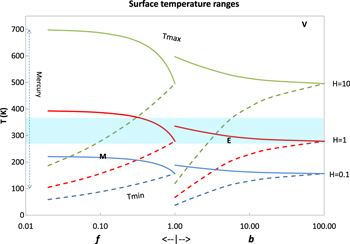
Figure 9. Combined chart of the extreme temperatures on locked planets in the H–f–b parameter space. The temperatures Tmin (dashed) and Tmax (solid) vs. the global redistribution parameter f (left side, assuming b = 0) and vs. the local transport parameter, b (right side, assuming f = 0). The liquid water range for 1 bar is shown by the shaded blue area. Letters indicate the terrestrial planets of the solar system; for Mars and Mercury, f is assigned the value of b.
Download figure:
Standard image High-resolution image7. The Biohabitable Domain in the Parameter Space
As described above, rather than using the spatial boundaries of the usual HZ, we define the range of surface temperatures allowing liquid water and the evolution of organic life, that is, complex organic molecules. The lower temperature boundary is obviously the freezing point of water, which only slightly depends on the pressure. The upper temperature boundary would be the highest temperature allowing complex organic molecules and life. On Earth, extremophiles near hydrothermal vents have been observed to survive and multiply at temperatures as high as ∼400 K,7 but much higher temperatures would be inimical to complex organic molecules and processes. Depending on the atmospheric pressure, this may be lower or higher than the temperature allowing liquid water. Conservatively, we take the temperature range allowing the evolution of life to be 273 K < T < 373 K. Minor variations of the upper boundary would slightly alter the range for the heating factor (Equation (18)), but would not substantially change our results.
Biohabitability requires the coldest region on the planet's surface to remain below the upper limit, namely Tmin < 373 K, and the hottest region to stay above freezing, that is, Tmax > 273 K. Note, however, that high salinity, water trapping and runaway warming or glaciation may modify these values, as discussed above. In terms of the heating factor H and the global redistribution parameter f, this condition can be written as

Combining these two conditions with Equations (14) and (15) gives

This range is shown in Figure 12 below. As H = Hgs, these relations may be transformed into a condition on the greenhouse heating (or equivalently, on the optical depth τLW) as a function of insolation, or, for a given host luminosity, as a function of the distance from the host. With Equation (12), the boundaries in Equation (19) can be written in the form
The two frames of Figure 10 show the biohabitability ranges of the greenhouse factor for two values of host star luminosity. For clarity, instead of the greenhouse factor Hg, we plot τLW = Hg–1 versus the planet's distance from its host star. The allowed range corresponding to Equation (20) is the vertical span between the curves of highest possible greenhouse factor (red curves) and minimal value (blue) for a fixed value of the redistribution parameter f.
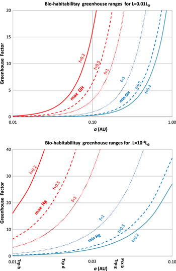
Figure 10. Maximal (red) and minimal (blue) biohabitable zone boundaries of the greenhouse factor (τLW = Hg–1) vs. semimajor axis, for three values of the heat redistribution parameter: f = 0.2 (solid), 0.5 (dashed), and 1 (dotted). The host luminosity is assumed to be L = 10−4 L⊙ (lower frame) and L = 0.01 L⊙ (upper frame). The locations of Proxima Cen b and three of the Trappist-1 planets are marked on the x-axis of the lower frame.
Download figure:
Standard image High-resolution imageThe luminosity used in the lower frame of Figure 10 is of the order of that of Trappist-1,8 hence, the orbital distances of the planets are indicated on the horizontal axis of that frame. For example, for Trappist-1d, the biohabitable range with a redistribution of f = 0.5 is 2 < τLW < 30, significantly larger than in the isothermal case (f = 1), where 4 < τLW < 15.
Equation (19) may be written in terms of the atmospheric heating and the insolation,
The corresponding ranges of the atmospheric heating factor can be seen in Figure 11, which shows the same boundaries as Figure 10 but in the parameter space defined by the atmospheric heating versus the insolation (calculated with the bolometric luminosity). As in the previous example, the biohabitable range for Trappist-1d with redistribution f = 0.5 is 0.3 < Hatm < 6, while the analogous range in the isothermal case is only 0.7 < Hatm < 2.5.

Figure 11. Maximal (red) and minimal (blue) biohabitable zone boundaries of the atmospheric heating factor vs. insolation, for three values of the heat redistribution parameter: f = 0.2 (solid), 0.5 (dashed), and 1 (dotted). The locations of Proxima Cen b and three of the Trappist-1 planets are marked on the x-axis.
Download figure:
Standard image High-resolution imageFigure 11 shows that in a significant part of the parameter space, spanned by the atmospheric properties (heating factor) and insolation, temperatures supporting liquid water and organic molecules may exist at least on part of the surface of locked planets. The size of this domain in the parameter space is smaller for nearly isothermal planets and significantly increases when global heat transport is less efficient.
Equations (18)–(19) also define the biohabitable range of the heating factor, as a function of the global redistribution parameter, as shown in Figure 12. For example, for f = 0.2, Equation (19) gives 0.24 < H < 14. This is consistent with Figure 4: on the curve H = 0.3, the highest temperature Tmax is barely above 273 K, while for the curve H = 10, the lowest temperature Tmin is just below 373 K.

Figure 12. Biohabitable ranges of the heating factors vs. f. Solid curves denote H, dashed ones Hatm. Upper curves indicate the maximal value, beyond which the planet is too hot, lower ones indicate the minimal value, below which the planet is too cold. Letters indicate the terrestrial planets in the solar system.
Download figure:
Standard image High-resolution imageAlthough the vertical lines in Figure 11 give the biohabitable range of the atmospheric heating factor for a fixed insolation, analogously to Equation (18), we may define the boundaries of the biohabitable domain for varying insolations. Combining Equation (13) with the spatial boundaries of the habitable zone gives an insolation-independent condition in the parameter space defined by the heat redistribution parameters and the atmospheric heating factor. If we adopt the boundaries in the classical HZ, e.g., for the inner edge the insolation of Venus and the outer edge at the insolation of Mars, the insolation relative to Earth is in the range 0.52 < s < 2.3 (cf., the habitable zone boundaries and their dependence on the atmospheric pressure and composition; Froget 2013; Vladilo et al. 2015). Since Hatm = Hs−1 we have
where Hmin and Hmax are the lowest and highest values of the heating factor (for a given value of f) in Equation (19) that permit liquid water and organic molecules to exist at some point of the surface of a tidally locked planet. Substituting the Venus-to-Mars HZ limits in Equation (19) gives

A similar analysis can be done for the LHT parameter (b). When 1 < b < 10, a condition on H analogous to Equation (19) may be calculated numerically using Equation (10), giving modified temperature ranges, as shown in Figure 13. For large LHT, b ≫ 10, as well as for f ∼ 1, the planet is isothermal. In that case, Equation (17) can be substituted in Equation (18), yielding 0.93 < H < 3.2.
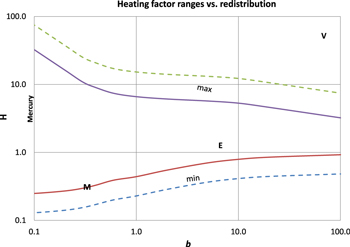
Figure 13. Biohabitable ranges of the heating factors vs. b. Solid curves denote H, dashed ones represent Hatm. The lower curves indicate the minimum value, below which the planet is too cold. The upper curves indicate the maximum value of H or Hatm, beyond which the planet is too hot (see text). Letters indicate the terrestrial planets in the solar system.
Download figure:
Standard image High-resolution imageSimilarly, for the atmospheric heating factor, a condition analogous to Equation (21) may be calculated numerically when 1 < b < 10, by using Equation (10). For b > 10 (as well as for f ∼ 1), the planet is nearly isothermal and Equation (17) gives 0.40 < Hatm < 6.15.
The upper curves (maximum values of the heating factors) in Figure 13 are calculated with the conservative night hemisphere temperatures (dotted curves in Figure 8).
The biohabitable constraints on the heating factor may be used to constrain the allowed range of atmospheric heating factor for a specific planet. For example, consider Proxima Cen b. Since Proxima Cen b has s = 0.65, substituting Hatm = Hs−1 in Equation (18) gives

As in Figure 9, we note that a large fraction of the Hatm−f or Hatm−b parameter space apparently supports liquid water and biohabitability on part of the planet's surface. This is true also for particular planets, as seen in Figure 14 for Proxima Cen b.
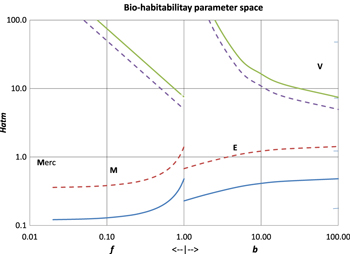
Figure 14. Combined chart of the conservative (273 K < T < 373 K) life-supporting temperature domain in the diagram of the atmospheric heating factor Hatm vs. the heat redistribution parameters. Left panel: Hatm vs. the global parameter (0 < f < 1). Solid curves denote the boundaries of the biohabitable domain (Equation (22)). Right panel: Hatm vs. the local transport parameter (1 < b < 100) with f = 0. The dashed curves refer to Proxima Cen b (Equation (23)). Letters indicate the terrestrial planets of the solar system (for Mars and Mercury, the f coordinate is taken as the value of b).
Download figure:
Standard image High-resolution image8. Biosignatures of M-dwarf Planets
The condition for life is often considered as liquid water on the planet surface. We have added the biotic temperature constraint, which may narrow the life-supporting region. In the previous section, we have charted the parameter space of tidally locked M-dwarf planets, showing that such planets can have liquid water and life-supporting local surface temperatures for a wide range of atmospheric properties. On the other hand, as has been pointed out, liquid water may actually be absent even on planets within the HZ, due to processes such as water trapping, greenhouse runaway evaporation, snowball runaway, limit cycling, or atmosphere erosion.
Liquid water may be a precursor of photosynthesis and atmospheric oxygen, also on planets of M stars (e.g., Gale & Wandel 2017). Spectral information about the planet's atmosphere may assess the presence of life, by identifying atmospheric biosignatures. Although a large abundance of water vapor in the atmosphere of a planet may well indicate an ocean or liquid water in a limited part of the surface, oxygen in the atmosphere is not necessarily a biotic indicator. Oxygen-rich atmospheres may evolve on M-dwarf planets by abiotic processes, giving a false-positive oxygen signature (Domagal-Goldman et al. 2014; Harman et al. 2015; Luger & Barnes 2015). Oxygen may be produced by abiotic processes such as photolysis of water or pre-main-sequence evolution of the M-dwarf host (Tian 2009; Tian et al. 2014; Wordsworth & Pierrehumbert 2014). However, massive photolysis also has a spectral signature, as it would produce detectable byproducts (Meadows et al. 2016) such as O4. To associate oxygen absorption features with photosynthesis, it would be necessary to back up oxygenic signatures with other biomarkers (Seager et al. 2016) such as CHN and CH4, or exclude the water photolysis mechanism by detecting significant quantities of non-condensing gases such as N2. A relatively robust potential biosignature is considered to be the detection of oxygen (O2) or ozone (O3) simultaneously with methane (CH4) at levels indicating fluxes from the planetary surface in excess of those that could be produced abiotically. For example, simultaneous detection of methane, ozone, and O2 may exclude abiotic production (Domagal-Goldman et al. 2014).
If the evolution of life on Earth is typical, a high level of oxygen in the atmosphere is reached 2–3 Gyr after the appearance of early life. As many red dwarfs are older than our Sun, and as shown in the previous chapters, a wide range of atmospheres allow liquid water and organic life within the HZ of M dwarfs, it is not unlikely that a large fraction of planets in the HZ of M stars have oxygen-rich atmospheres of biotic origin.
Oxygen and other biosignatures may be detected in transiting exoplanets by observing atmospheric absorption lines in the transmitted spectrum of the host star. The smaller the host star, the easier this can be accomplished, so M dwarfs are the most suitable candidates. TESS is likely to find dozens of transiting Earth or super-Earth-size planets possibly close enough for spectroscopic biosignature detection by JWST (Seager 2015).
By the same argument, it would be even easier to detect biomarkers in planets of white dwarfs (Loeb & Maoz 2013). Due to their low luminosity, HZs of white dwarfs are relatively small and hence planets in the HZ of a white dwarf are also likely to be tidally locked. It is likely that as much as 30% of the white dwarfs have planetary systems (Zuckerman et al. 2010). However, because of the small dimensions of the host, transiting planets around white dwarfs may be less frequent, unless the planetary material is extended, as in the case of WD 1145+017 (Vanderburg et al. 2015). Planets near a white dwarf would probably not be able to maintain their water and atmosphere over the violent past of their host, but planets may migrate from a larger distance or accrete new water from the debris of the parent planetary nebula phase.
9. The Abundance of Biotic Planets
How abundant are habitable M-dwarf planets that actually have biotic oxygen? What is the fraction of planets with liquid water that develop oxygenic photosynthesis and detectable levels of oxygen? In order to tackle these questions, we need first to estimate the abundance of candidates. Then, using the latest Kepler statistics, we estimate the relative abundance of planets for which we might find such biosignatures.
Assuming that biotic life is long lived, as on Earth (∼4 Gyr for monocellular life), the number of biotic planets can be expressed in a Drake-like equation (Wandel 2015),

where N* is the number of stars in the Galaxy, Fs is the fraction of stars suitable for evolution of life, and FEHZ is the fraction of such stars that have Earth-size planets within their HZ. The last parameter, Fb, is the (yet unknown) biotic probability namely that a habitable planet actually becomes biotic within a few billion years. The average distance db between biotic neighbor planets can then be shown to be (Wandel 2015, 2017a, 2017b)

where  is the stellar number density in the solar neighborhood. For red dwarf stars, n* ∼ 0.2 pc−3 and Fs ∼ 0.7 (Winters et al. 2015; Henry et al. 2006).
The abundance factor FEHZ of Earth-size habitable planets can be estimated from the Kepler data (e.g., Dressing & Charbonneau 2015). Within a conservative definition of the HZ (based on the moist greenhouse inner limit and maximum greenhouse outer limit), there are  Earth-size planets (1–1.5 R⊕) and
  super-Earths (1.5–2 R⊕) per red dwarf. With broader HZ boundaries (present Venus–Mars insolation), these estimates increase by ∼50%. This gives a minimum of 0.09 Earth-size planets to a maximum of 0.75 habitable Earth- or super-Earth-size planets per red dwarf. Hence, FEHZ ∼ 0.1–0.75, depending on the definition of the HZ.
Substituting these values into Equation (25) gives

For example, assuming one in ten Earth-size habitable planets of M stars becomes biotic (Fb = 0.1), Equation (26) gives db ∼ 1.5–3 pc. The results of the previous sections could place the actual value of FEHZ (the fraction of Earth-sized planets in the biohabitable zone) closer to unity, as well as increase the expected value of Fb.
The expected number of biotic planets within a distance d may be derived from Equation (25) by substituting the values of n* and Fs,

Figure 15 shows the expected number Nb as a function of the distance and the product FEHZFb. Biohabitability, as defined in Sections 6–7 (surface temperatures supporting liquid water and organics), allows the evolution of oxygenic photosynthesis9 (Gale & Wandel 2017; see also footnote 1) and an oxygenic biosignature. This gives a direct relation between the observed number of planets with oxygenic signatures and the biotic probability Fb, with the caveat of abiotic false-positive oxygen signatures discussed earlier.
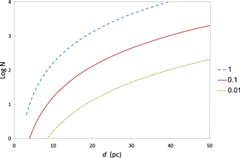
Figure 15. Number of red dwarf planets with oxygenic biosignatures expected within a distance d, for several values of the product FEHZFb (marked on the right), where Fb is the biotic probability (see text) and FEHZ is the fraction of M stars with Earth-sized HZ planets.
Download figure:
Standard image High-resolution imageTESS, scheduled for launch in 2018, is projected to find hundreds of transiting Earth-to-super-Earth size planets, many of them in the HZs of nearby M dwarfs (Ricker et al. 2015; Seager 2015). By geometrical and statistical arguments, only a small fraction of the habitable red dwarf planets are expected to be transiting. The transiting angular range depends mainly on the size of the host star (R*) and the distance of the planet from its host star (a). For R* ≪ a, the transiting probability is ∼R*/a, which for planets in the HZ of a red dwarf turns out to be 1%–2%. Hence, we need to find a large enough number of transiting planets in order to produce a statistically significant subset of candidates.
In order to assess the number of candidates, given the spectral signature detection distance appropriate for the particular method and platform, we can determine the number of expected candidates by calculating the cumulative number of biotic planets as a function of distance (Wandel 2017b).
From Equation (27) and in Figure 15 we can, substituting Fb = 1, calculate the expected number of candidate planets within a given distance (the biosignature detection range) and subsequently estimate the number of transiting planets. For example, assuming that the M-dwarf habitability fraction is FEHZ = 0.5, one could expect ∼2000 habitable planets of red dwarfs within 30 pc. With a transiting probability of 1%–2%, TESS can be expected to detect 20–40 transiting ones.10 As an example, let us assume that out of 30 candidates, JWST finds oxygen signatures in 20 planets, and half of them have other supporting biosignatures. One could then estimate the biotic probability to be Fb ∼ 0.3 ± 0.05. As JWST will probably be marginally capable of detecting biosignatures and may need long exposures, at least as a pilot it would be better to concentrate on a short list of best candidates (nearby systems with several planets in the biohabitable zone, such as Trappist-1).
10. Summary
We use a simple climate model in order to investigate the surface temperature distribution and habitability of gravitationally locked planets, taking into account irradiation, albedo, horizontal heat transport, and atmospheric effects such as screening and the greenhouse effect. We show that HZ planets of M-dwarf stars may have a surface temperature distribution supporting liquid water and complex organic molecules on at least part of their surface, for a wide range of atmospheric properties and heat transport. We apply these results to Proxima Cen b and to the Trappist-1 system and discuss the implications for searching for oxygen and other biosignatures in transiting habitable planets of nearby M dwarfs (cf., Gardner et al. 2006; Seager 2015). From the Kepler data, we estimate that within 30 pc, TESS may find ∼10–40 transiting candidates. We show how detecting a few planets with atmospheric oxygen one may estimate the abundance of photosynthesis and biotic planets (or an upper limit, if none are detected), providing evidence for life (Spiegel & Turner 2012).
The author thanks an anonymous referee for careful reviewing and useful comments, Joe Gale for useful discussions, and the organizers of the Astrobiology 2017 and 51ESLAB meetings, where parts of this work have been presented.
Footnotes
- 1
Wandel, A., & Gale, J. 2017, IAU commission F3 meeting Astrobiology, https://www.youtube.com/watch?v=BtDv-o0b_0c
- 2
Alternatively, S may be expressed in the form
 , where T* and R* are the host star's surface temperature and radius, respectively. The temperature can then be expressed in the form Teq = T*(R*/2a)1/2(1 − A)1/4.
 - 3
The combined effect of a vertical energy exchange with the atmosphere and an atmospheric horizontal circulation can be shown to have the approximate effect of horizontal heat redistribution; see, e.g., Koll & Abbot (2016).
- 4
For an optically thick atmosphere, Hg ∼ τLW, hence Equation 2(a) gives
. Pierrehumbert's relation is , where β depends mainly on the molecular weight. Typical values for N2 or CO2 atmospheres are β ∼ 0.1–0.3. - 5
Obviously, global heat transport is also determined by the atmospheric and planetary properties, as may be calculated by GCMs, but the relation is less explicit, depending on the vertical transport and on global circulation currents.
- 6
See Section 6 for the definition of biohabitability.
- 7
- 8
The bolometric luminosity of Trappist-1a is 0.0052L⊙, but as most of it is in the long wavelength (visual luminosity only 3.7 × 10⁻⁶ L⊙), the radiation flux at the surface depends on τLW and may significantly lower; e.g., if τLW = 3, it would be ∼10−4L⊙.
- 9
For gravitationally locked planets, photosynthesis may exclude the regime where only the night hemisphere is biohabitable, unless the atmosphere is sufficiently dense to scatter light from the day hemisphere.
- 10
Applying the above range 0.1 < FEHZ < 0.75 would give an expectation of 4–60 transiting M-dwarf planets, but conservatively we narrow this range to 10–40.


