Wide-spectral-band Nuller Insensitive to Finite Stellar Angular Diameter with a One-dimensional Diffraction-limited Coronagraph

We use the pupil coordinates α = (α, β) normalized by the telescope diameter D and the focal coordinates x = (x, y) normalized by λ/D, where λ donates the light wavelength to be observed: the normalization factors D and λ/D scale with the magnification factors of pupils and images. The following function definitions work throughout this paper:

$$\begin{eqnarray}&&\mathrm{rect}\left[v\right]=\left\{\begin{array}{l}1\quad \left(\left|v\right|\lt \displaystyle \frac{1}{2}\right)\\ \displaystyle \frac{1}{2}\quad \left(\left|v\right|=\displaystyle \frac{1}{2}\right)\\ 0\quad \left(\left|v\right|\gt \displaystyle \frac{1}{2}\right)\end{array}\right.\end{eqnarray} \tag{ 1 }$$

and

$$\begin{eqnarray}&&\mathrm{sinc}\left(x\right)=\displaystyle \frac{\sin \left(\pi x\right)}{\pi x}.\end{eqnarray} \tag{ 2 }$$

In the 1DDLC, the focal-plane mask modulates the amplitudes and phases of light so that the light from the on-axis source has no transmittance through the Lyot Stop and that light from off-axis sources transmits through the Lyot Stop. The 1DDLC has the following pupil aperture function P( α ), Lyot stop aperture function L( α ), and focal-plane mask function M( x ):

$$\begin{eqnarray}&&P({\boldsymbol{\alpha }})=L({\boldsymbol{\alpha }})=\mathrm{rect}\left[\alpha \right]\mathrm{rect}\left[\beta \right]\end{eqnarray} \tag{ 3 }$$

and

$$\begin{eqnarray}&&M({\boldsymbol{x}})=a\left(1-2\mathrm{sinc}\left(2x\right)\right),\end{eqnarray} \tag{ 4 }$$

where the constant factor a takes 0.697... so that $\left|M({\boldsymbol{x}})\right|\leqslant 1$. We see how the coronagraph works using the following orthonormal complete base functions $\left\{{b}_{\mathrm{kl}}\left({\boldsymbol{\alpha }}\right)\left|k,l\in {\mathbb{Z}}\right.\right\}$:

$$\begin{eqnarray}&&{b}_{\mathrm{kl}}\left({\boldsymbol{\alpha }}\right)=P({\boldsymbol{\alpha }}){e}^{2\pi i\left(k\alpha +l\beta \right)}.\end{eqnarray} \tag{ 5 }$$

Expanding an arbitrary pupil amplitude v( α ) on the pupil aperture with the base functions leads to the following expression:

$$\begin{eqnarray}&&v\left({\boldsymbol{\alpha }}\right)=\displaystyle \sum _{k=-\infty }^{\infty }\,\displaystyle \sum _{l=-\infty }^{\infty }{w}_{\mathrm{kl}}{b}_{\mathrm{kl}}\left({\boldsymbol{\alpha }}\right),\end{eqnarray} \tag{ 6 }$$

where

$$\begin{eqnarray}&&{w}_{\mathrm{kl}}={\int }_{-\infty }^{\infty }d\alpha {\int }_{-\infty }^{\infty }d\beta \ {b}_{\mathrm{kl}}{\left({\boldsymbol{\alpha }}\right)}^{* }v\left({\boldsymbol{\alpha }}\right).\end{eqnarray} \tag{ 7 }$$

The coronagraph defined by Equations (3) and (4) acts as the following linear transformation:

$$\begin{eqnarray}&&{w}_{\mathrm{kl}}\to a\left(1-{\delta }_{k0}\right){w}_{\mathrm{kl}},\end{eqnarray} \tag{ 8 }$$

where the symbol δ_kl means Kronecker delta. Hence, the coronagraph nulls the weights $\left\{{w}_{0l}\left|l\in {\mathbb{Z}}\right.\right\}$ and transmits the weights $\left\{{w}_{\mathrm{kl}}\left|k,l\in {\mathbb{Z}},k\ne 0\right.\right\}$ multiplying the constant factor a of the focal-plane mask.

We can express a tilt aberration of tiny-amount direction cosines of (Δθ_x , Δθ_y ) on the pupil plane as the following expression:

$$\begin{eqnarray}&&{v}_{\mathrm{tilt}}\left({\boldsymbol{\alpha }}\right)=P({\boldsymbol{\alpha }}){e}^{2\pi i\left({\rm{\Delta }}{\theta }_{x}\alpha +{\rm{\Delta }}{\theta }_{y}\beta \right)}\end{eqnarray} \tag{ 9 }$$

$$\begin{eqnarray}&&\sim {b}_{00}\left({\boldsymbol{\alpha }}\right)+2\pi {iP}({\boldsymbol{\alpha }})\left({\rm{\Delta }}{\theta }_{x}\alpha +{\rm{\Delta }}{\theta }_{y}\beta \right).\end{eqnarray} \tag{ 10 }$$

The coronagraph defined by Equations (3) and (4) works to the input amplitude ${v}_{\mathrm{tilt}}\left({\boldsymbol{\alpha }}\right)$ as the following transformation:

$$\begin{eqnarray}&&{v}_{\mathrm{tilt}}\left({\boldsymbol{\alpha }}\right)\to {v}_{\mathrm{tilt}}^{\mathrm{out}}\left({\boldsymbol{\alpha }}\right)=2\pi {iaP}({\boldsymbol{\alpha }}){\rm{\Delta }}{\theta }_{x}\alpha .\end{eqnarray} \tag{ 11 }$$

The Fourier transform of the output amplitude on the Lyot stop yields focal amplitude u( x ) on the detector plane:

$$\begin{eqnarray}&&u({\boldsymbol{x}})={\int }_{-\infty }^{\infty }d\alpha {\int }_{-\infty }^{\infty }d\beta \ {v}_{\mathrm{tilt}}^{\mathrm{out}}\left({\boldsymbol{\alpha }}\right){e}^{-2\pi i\left(x\alpha +y\beta \right)}.\end{eqnarray} \tag{ 12 }$$

The pupil amplitude $\ {v}_{\mathrm{tilt}}^{\mathrm{out}}\left({\boldsymbol{\alpha }}\right)$ is an odd function about the coordinate α and an even function about the coordinate β. Since the Fourier transform keeps parity (whether the function is even or odd) of operand functions, the focal amplitude u( x ) on the detector plane is also an odd function about the coordinate x and an even function about the coordinate y:

$$\begin{eqnarray}\begin{array}{rcl}u(-x,y) & = & -u(x,y),\\ u(x,-y) & = & u(x,y).\end{array}\end{eqnarray} \tag{ 13 }$$

Since the pupil amplitude $\ {v}_{\mathrm{tilt}}^{\mathrm{out}}\left({\boldsymbol{\alpha }}\right)$ is proportional to the magnitude of the tilt aberration Δθ_x , the intensity of the leak on the detector plane is proportional to ${\left({\rm{\Delta }}{\theta }_{x}\right)}^{2}$. Hence, the 1DDLC system shows the second-order sensitivity to the tilt aberration due to the nonzero diameter of the central stars.

When the observation wavelength λ differs from the design wavelength λ_d of the focal-plane mask, we must change the mask function from Equation (4) to the following:

$$\begin{eqnarray}&&{M}_{{\rm{\Lambda }}}({\boldsymbol{x}})=a\left(1-2\mathrm{sinc}\left(2{\rm{\Lambda }}x\right)\right),\end{eqnarray} \tag{ 14 }$$

where we defined that Λ = λ/λ_d . Since the deviation M_Λ( x ) − M₁( x ) of the mask function from the ideal case (Λ = 1) is an even function about x and y, the leak amplitude v(x, y) caused by this deviation is also an even function about x and y on the focal plane after the Lyot stop:

$$\begin{eqnarray}\begin{array}{rcl}v(-x,y) & = & v(x,y),\\ v(x,-y) & = & v(x,y).\end{array}\end{eqnarray} \tag{ 15 }$$

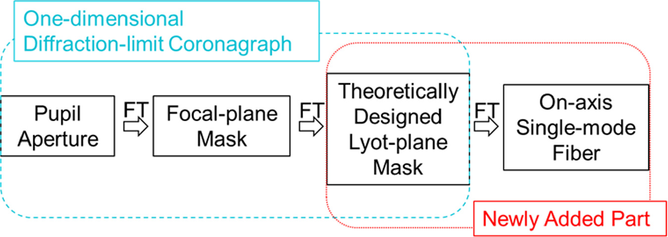
The new method consists of the 1DDLC (Appendix 2.1) and newly added parts: a theoretically designed Lyot-plane mask and a single-mode fiber located at the on-axis point (Figure 1). The 1DDLC transmits the stellar leaks (due to nonzero stellar angular diameter and spectral bandwidth) to its pupil plane where the Lyot stop is located (Lyot plane). We design the Lyot-plane mask so that it removes these leaks achromatically and delivers sufficient planetary light to spectrometers through the on-axis single-mode fiber.

Zoom In Zoom Out Reset image size

We focus on the parity of the amplitude-spread functions to design the appropriate Lyot-plane mask and build the new method. The Fraunhofer diffraction integral of a pupil function is a Fourier transform, which scales with the wavelength of light. This scaling by the wavelengths limits the bandwidths of phase-mask coronagraphy to narrow bands. Parity is a concept independent of the scales of the focal-plane amplitude-spread function, in other words, the wavelength of light, thus it is worth focusing on the parity of the amplitude-spread functions to design a method less dependent on the wavelength of light.

We can write any amplitude-spread function on pupil and focal planes as the sum of its four different components. The first component is a function that is an even function for the first and second arguments (we refer to this as EE component), the second is even for the first argument but is odd for the second arguments (EO component), the third is odd for the first and even for the second arguments (OE component), and the fourth is odd for both arguments (OO component). Formally, we can expand an arbitrary amplitude-spread function f(s, t) as a sum of the four components concerning their parities as follows:

$$\begin{eqnarray}&&f(s,t)={f}_{\mathrm{EE}}(s,t)+{f}_{\mathrm{OE}}(s,t)+{f}_{\mathrm{EO}}(s,t)+{f}_{\mathrm{OO}}(s,t),\end{eqnarray} \tag{ 16 }$$

where

$$\begin{eqnarray}&&{f}_{\mathrm{EE}}(s,t)=\displaystyle \frac{f(s,t)+f(-s,t)+f(s,-t)+f(-s,-t)}{4},\end{eqnarray} \tag{ 17 }$$

$$\begin{eqnarray}&&{f}_{\mathrm{OE}}(s,t)=\displaystyle \frac{f(s,t)-f(-s,t)+f(s,-t)-f(-s,-t)}{4},\end{eqnarray} \tag{ 18 }$$

$$\begin{eqnarray}&&{f}_{\mathrm{EO}}(s,t)=\displaystyle \frac{f(s,t)+f(-s,t)-f(s,-t)-f(-s,-t)}{4},\end{eqnarray} \tag{ 19 }$$

$$\begin{eqnarray}&&{f}_{\mathrm{OO}}(s,t)=\displaystyle \frac{f(s,t)-f(-s,t)-f(s,-t)+f(-s,-t)}{4},\end{eqnarray} \tag{ 20 }$$

and the coordinates (s,t) represents the focal coordinates (x,y) or the pupil coordinate (α, β). The subscripts p₁ p₂ in the notation of the above components ${f}_{{{\rm{p}}}_{1}\ {{\rm{p}}}_{2}}(s,t)$ (${{\rm{p}}}_{1},\ {{\rm{p}}}_{2}\in \left\{{\rm{E}},{\rm{O}}\right\}$) express the parity (E: even, O: odd) about the first argument s and the second arguments t, respectively. Since the Fourier transform does not change the parity of an arbitrary function, Fraunhofer diffraction between the focal and pupil plane preserves the parities of the light amplitudes. We can achieve at least the fourth-order null by erasing the leak amplitude of the least-order term of tilt aberration; this least-order term of tilt aberration contains only the OE component (Section 2.1). The deviation of the actual wavelength from the design wavelength of the focal-plane mask creates only the EE component (Section 2.1).

In the new method, we use a single-mode fiber such that the fiber center matches the focal-plane origin ${\boldsymbol{x}}=\left(0,0\right);$ we assume that the stellar center matches the origin if no starlight-removing optical device including coronagraph exists. We assume that the transmission mode function g( x ) of the single-mode fiber is a function with only an EE component. We can calculate the fiber-transmitted intensity I using the following expression (Wagner & Tomlinson 1982):

$$\begin{eqnarray}&&I={\left|{\int }_{-\infty }^{\infty }{dx}{\int }_{-\infty }^{\infty }{dy}\ g(x,y)f(x,y)\right|}^{2}.\end{eqnarray} \tag{ 21 }$$

Substituting Equations (16)–(21) leads to the intensity transmitted through the single-mode fiber for an arbitrary focal amplitude $f\left({\boldsymbol{x}}\right)$ as follows:

$$\begin{eqnarray}\begin{array}{rcl}I & = & \left|{\int }_{-\infty }^{\infty }{dx}{\int }_{-\infty }^{\infty }{dy}\ g(x,y)\left({f}_{\mathrm{EE}}(x,y)\right.\right.\\ & & {\left.\left.+{f}_{\mathrm{OE}}(x,y)+{f}_{\mathrm{EO}}(x,y)+{f}_{\mathrm{OO}}(x,y)\right)\right|}^{2}\\ & = & {\left|{\int }_{-\infty }^{\infty }{dx}{\int }_{-\infty }^{\infty }{dy}\ g(x,y){f}_{\mathrm{EE}}(x,y)\right|}^{2},\end{array}\end{eqnarray} \tag{ 22 }$$

where we used the odd-function nature of f_OE(x, y), f_EO(x, y), and f_OO(x, y). Equation (22) shows that the amplitudes belonging to the OE, EO, and OO components fail to transmit the single-mode fiber located at the origin.

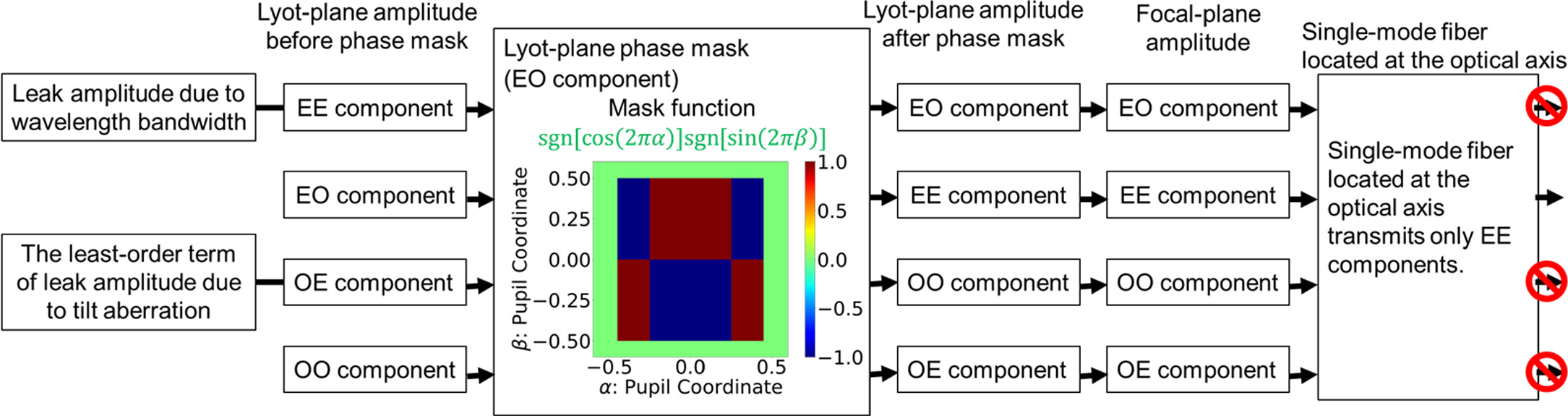
To achieve the wideband fourth-order null by eliminating OE components (the leak from the least-order term of the tilt aberration) and EE components (the leak due to the wavelength deviation from the design wavelength), we need to change the OE and EE components to components other than EE components. Multiplying a function that has only an EO component to the functions of OE and EE components leads to the function of OO and EO components, respectively; this multiplication satisfies the above requirement. Hence, the mask function of the Lyot-plane phase mask must include only an EO component to achieve the wideband fourth-order null. We compiled how the new concept works to remove undesirable leak amplitudes as a block diagram in Figure 2.

Zoom In Zoom Out Reset image size

The additional requirement for the Lyot-plane phase mask concerns the planetary throughput. To secure the planetary throughput via the single-mode fiber located at the optical axis, we can use the following sinusoidal modulation pattern with only an EO component:

$$\begin{eqnarray}\begin{array}{rcl}{s}_{{qr}}^{\mathrm{sinu}}\left({\boldsymbol{\alpha }}\right) & = & \cos \left(2\pi q\alpha \right)\sin \left(2\pi r\beta \right)\\ & = & \displaystyle \frac{1}{4i}\left({e}^{2\pi {iq}\alpha }+{e}^{-2\pi {iq}\alpha }\right)\left({e}^{2\pi {ir}\beta }+{e}^{-2\pi {ir}\beta }\right),\end{array}\end{eqnarray} \tag{ 23 }$$

where q and r are the design parameters of the mask. The modulation pattern ${s}_{{qr}}^{\mathrm{sinu}}\left({\boldsymbol{\alpha }}\right)$ works as a two-dimensional diffraction grating with nonzero diffraction efficiency for only the diffraction orders of (1, 1), (−1, 1), (1, − 1), and (−1, − 1). The single peak of the focal amplitude exists at the optical axis and transmits the single-mode fiber efficiently (Figure 3).

Zoom In Zoom Out Reset image size

Adopting the following rectangular-wave-like phase-modulation pattern improves the planetary throughput and the easiness of manufacturing the mask compared to the case with the sinusoidal pattern:

$$\begin{eqnarray}\begin{array}{rcl}{s}_{{qr}}^{\mathrm{rect}}\left({\boldsymbol{\alpha }}\right) & = & \mathrm{sgn}\left[\cos \left(2\pi q\alpha \right)\right]\mathrm{sgn}\left[\sin \left(2\pi r\beta \right)\right],\end{array}\end{eqnarray} \tag{ 24 }$$

where the symbol $\mathrm{sgn}\left[...\right]$ means the sign function. We define the sign function as follows:

$$\begin{eqnarray}&&\mathrm{sgn}\left[z\right]=\left\{\begin{array}{l}-1\,\,\left(z\lt 0\right)\\ 0\,\,\left(z=0\right)\\ 1\,\,\left(z\gt 0\right).\end{array}\right.\end{eqnarray} \tag{ 25 }$$

Since the modulation pattern ${s}_{\mathrm{qr}}^{\mathrm{rect}}\left({\boldsymbol{\alpha }}\right)$ takes the values of only −1 or 1 (i.e., e^{π i} or e⁰ⁱ ), the modulation includes only π-radian phase modulation, resulting in the high planetary throughput and the mask-manufacturing simplicity. See also Appendix concerning another expression of the Lyot-plane phase mask function.

For a realistic performance evaluation of the new concept, we have to apply the following instrumental conditions. (1) We use the 1DDLC summarized in Section 2.1. (2) We utilize the Lyot-plane phase-mask function shown in Equation (24) with the following parameters: (q, r) = (1, 1). Because we are most interested in the performance of the case with the innermost planetary angular separation from the perspective of complementarity to other coronagraphs, we adopt the above mask parameters. (3) We assume the following transmission mode function of the single-mode fiber located at the optical axis of the final focal plane: g(x, y) = sinc(x)sinc(y). The heart of this assumption is only the parity of the transmission mode function. We are not interested in the precise functional form of the transmission mode function here.

To evaluate the theoretically achievable performance of the new concept, we perform a numerical simulation with the following setup. The simulation includes the following parameters expressing different simulation cases.

• 1.  
  The spectral bandwidth $\tfrac{{\rm{\Delta }}\lambda }{{\lambda }_{c}}$ serves as a simulation parameter; we assume that the light source has a center wavelength λ_c of 700 nm and the uniform spectral distribution from ${\lambda }_{c}-\tfrac{{\rm{\Delta }}\lambda }{2}$ to ${\lambda }_{c}+\tfrac{{\rm{\Delta }}\lambda }{2}$, where Δλ denotes a wavelength width.
• 2.  
  We use the stellar angular diameter as a simulation parameter; we assume the uniform intensity distribution of the light source within its angular diameter.
• 3.  
  We take the planetary x- and y-directional separation angles (θ_x , θ_y ) (normalized by λ_c /D) as simulation parameters.

For the numerical Fourier transform, we use the same calculation method as the one shown in Appendix B of the paper Itoh & Matsuo (2022).

Figure 4 shows the simulation result concerning the planetary throughput. The left panel of Figure 4 indicates the planetary throughputs (including the fiber-coupling efficiency) over different planetary separations assuming monochromatic light. Our original design philosophy of the Lyot-plane mask expected that the throughput map of the left panel of Figure 4 has peak values when

$$\begin{eqnarray}\begin{array}{rcl}\left({\theta }_{x},{\theta }_{y}\right) & = & (q,r),(-q,r),(q,-r),(-q,-r)\\ & = & (1,1),(-1,1),(1,-1),(-1,-1).\end{array}\end{eqnarray} \tag{ 26 }$$

However, the result in the left panel of Figure 4 shows that the throughput map peaks when

$$\begin{eqnarray}&&\left({\theta }_{x},{\theta }_{y}\right)=(Q,R),(-Q,R),(Q,-R),(-Q,-R),\end{eqnarray} \tag{ 27 }$$

where (Q, R) ∼ (1.125, 0.750); the peak value reaches about 11%. The right panel of Figure 4 shows the planetary throughputs for different spectral bandwidths. We can observe the constancy of the planetary throughputs against the change in the spectral bandwidth.

Zoom In Zoom Out Reset image size

Figure 5 shows the simulation result concerning the achievable raw contrast. In Figure 5, we can find that the new method can achieve the raw contrast of about 4 × 10⁻⁸ (Δλ/λ_c = 0.25) and 5 × 10⁻¹⁰ (Δλ/λ_c = 0.10) when the star has the angular diameter of 3 × 10⁻² λ_c /D. We can also see that in the monochromatic case (Δλ/λ_c = 0.00), the raw contrast seems proportional to the about sixth power of the stellar angular diameter. In the cases with nonzero spectral bandwidths, the raw contrast and the stellar diameters exhibit no simple power-law relations, but when we focus only on the region of the stellar angular diameters less than 3 × 10⁻² λ_c /D, the relation approximately obeys power laws with the power-law exponent of about two and the constant coefficients depending on the spectral bandwidths. On the other hand, when the stellar angular diameters overvalue 3 × 10⁻¹ λ_c /D, the raw contrasts have little dependency on the spectral bandwidth. When we focus only on the intermediate region, we can infer that, in this region, the relations have different power-law exponents depending on the spectral bandwidths.

Zoom In Zoom Out Reset image size

4.1.1. Factor-specific Discussion on the Planetary Throughput

4.1.2. Azimuthal-angle Dependency of Planetary Throughput

In Figure 4, we observe that the planetary throughput of this method has a nonuniform dependency on the azimuthal angle for a given radius of the planetary separation. We extracted and plotted the azimuthal-angle dependence of the planetary throughput in Figure 6. 

Zoom In Zoom Out Reset image size

Here, we discuss the impact of the nonuniform throughput on planetary detection and spectroscopic observation.

Planetary Detection—without anticipation of the planetary location, the azimuth dependence degrades the exploration efficiency (the left panel of Figure 6). However, from a practical point of view, how much additional time we need is a more important measure than the degradation rate of the exploration efficiency. In the right panel of Figure 6, we show that we can acquire an almost azimuthally homogeneous throughput with a throughput of about 18% by summing the four exposures with the image rotation by 0°, 45°, 90°, and 135°. Based on this scanning strategy, we can estimate the increase of the observation time Δt_p required for S/N = p in the following manner:

$$\begin{eqnarray}&&{\rm{\Delta }}{t}_{p}=(Q-1){t}_{p},\end{eqnarray} \tag{ 28 }$$

where the degradation rate Q of the observation efficiency satisfies Q = 4 (the number of exposures required for the complete azimuthal scan) and t_p denotes the observation time required for S/N = p in the case with no azimuth dependence of the throughput (Q = 1). Using the effective throughput τ (∼0.18 from the right panel of Figure 6) and the number of planetary photons that reach the telescope aperture per hour $\dot{n}$, we can express the requirement time t_p in the case with no degradation in the observation efficiency as follows:

$$\begin{eqnarray}&&{t}_{p}=\displaystyle \frac{{p}^{2}}{\tau \dot{n}},\end{eqnarray} \tag{ 29 }$$

where we ignored the photons of the stellar leak because the number of them falls less compared to the planetary photons thanks to the nuller's contrast-mitigation ability presented in Figure 5. In Table 1, we show per-an-hour numbers $\dot{n}$ of planetary photons that reach inside the telescope aperture for the possible target examples under a given condition (D = 6 m, λ_c = 700 nm, and Δλ/λ_c = 0.10) assuming detecting potentially habitable planets around different types of host star. Using the values $\dot{n}$ in Table 1, we can estimate the increase of the observation time Δt₅ required for S/N = 5 as follows:

$$\begin{eqnarray}&&\begin{array}{l}{\rm{\Delta }}{t}_{5}=\left\{\begin{array}{l}0.28\,\mathrm{hr}\ \ \left({T}_{\mathrm{eff}}=3900\,{\rm{K}}\right)\\ 0.32\,\mathrm{hr}\ \ \left({T}_{\mathrm{eff}}=3500\,{\rm{K}}\right).\end{array}\right.\end{array}\end{eqnarray} \tag{ 30 }$$

Hence, even though exposure time quadruples, for typical target system of the 1DDLC, the overall detection time to achieve that S/N = 5 remains under an hour To change the planetary azimuthal angle with respect to the coronagraphic instruments, for example, we can rotate the entire telescope around the optical axis (Gaudi et al. 2020) or use an image-rotation unit made with a Dove prism (Moreno et al. 2003).

Table 1. Typical Observation Requirement for Detecting Potentially Habitable Planets Around Different Types of Host Stars

Assumed Parameters				Calculated Values
Teff (K)	d (pc)	θ* (mas)	θ* (λc /D)	θsep (mas)	θsep (λc /D)	C	$\dot{n}$ (h−1)
3900	10	0.56	2.3 × 10−2	27	1.1	2.9 × 10−9	1500
3500	10	0.36	1.6 × 10−2	15	0.62	1.0 × 10−8	1300

Note. The effective temperature T_eff, distance d, and stellar angular diameter θ_* characterize the assumption of the host stars. The first, second, and third column in the table means the cases of an early-M dwarf (T_eff = 3900 K) and mid-M dwarf (T_eff = 3500 K), respectively. We referred to the values of the stellar physical radii R_* in Boyajian et al. (2012) to assume the values of θ_*. As values determining instrumental requirements, we show the planetary angular separation θ_sep, planet–star contrast ratio C, and the number of photons that reach the telescope aperture per hour after reflected at the planetary surfaces $\dot{n}$ (D = 6m, λ_c = 700nm, and Δλ/λ_c = 0.10) in the table. To evaluate θ_sep, we used the following equation determining the planet–star physical distance r_p such that the planet receives the same amount of radiation flux as the Earth: ${r}_{p}=(1\,\mathrm{au})\times ({R}_{* }/{R}_{\odot }){\left({T}_{\mathrm{eff}}/{T}_{\odot }\right)}^{2}$. The contrast C comes from the following equation assuming Earth-sized face-on planets: $C={A}_{g}{\left({R}_{\oplus }/{r}_{p}\right)}^{2}/\pi$, where A_g denotes the geometric albedo of the Earth. We derived $\dot{n}$ by multiplying the contrast C by the number of stellar photons that reach the telescope aperture per hour evaluated with Planck's law.

Download table as:  ASCIITypeset image

Possibility of a Calibration Method for Planetary Detection—the azimuth dependence of the planetary throughput may work as a key to further contrast mitigation through data analyses. The curves in Figure 6 show that the planetary signals have their inherent profile as functions of the azimuthal angles of the planetary separation. On the other hand, the stellar leak is constant for the change of the planetary azimuthal angle in principle. Hence, for example, we can expect that using the cross-correlation method between the model profile of the signal and measured data set along the azimuthal angles will lead to higher signal-to-noise ratios compared to ones expected from the raw contrast of Figure 5. A similar data filtering technique appears in observing mid-infrared thermal emissions emitted from Earth-like planets with nulling interferometer (Mennesson & Mariotti 1997), but the present one and nulling interferometers have a difference in the point that the present one will remove stellar leaks (speckle noises) while the nulling interferometers will remove exozodiacal emissions.

Spectroscopic Observation—after detecting the location of a promising target, we can use a fixed image-rotation angle optimized to the target to perform the spectroscopic observation with the highest throughput (11%). Since we need no image rotation during this observation mode, we can secure sufficient detected-photon number for each resolvable spectrum element with a practical integration time.

4.2.1. Mathematical Interpretation

The numerical simulation suggests that the raw contrast approximately obeys a linear combination of some power-law functions consistently to the following mathematical interpretation. Using Taylor expanding for functions with two variables, we can rewrite Equation (9) as the following expression:

$$\begin{eqnarray}&&{v}_{\mathrm{tilt}}\left({\boldsymbol{\alpha }}\right)=P({\boldsymbol{\alpha }})\displaystyle \sum _{N=0}^{\infty }\displaystyle \sum _{K=0}^{N}{g}_{K;N-K}(\alpha ,\beta ),\end{eqnarray} \tag{ 31 }$$

where

$$\begin{eqnarray}&&{g}_{K;N-K}(\alpha ,\beta )=\displaystyle \frac{{\left(2\pi i\right)}^{N}}{N!}\left(\displaystyle \genfrac{}{}{0em}{}{N}{K}\right){\left({\theta }_{x}\alpha \right)}^{K}{\left({\theta }_{y}\beta \right)}^{N-K}.\end{eqnarray} \tag{ 32 }$$

Since the function g_K;N−K (α, β) is a power function, the parity of the function g_K;N−K (α, β) concerning the arguments α and β match the parity as integers of power exponents K and N − K, respectively. Thus, only when K is even and N − K is odd, the term g_K;N−K (α, β) transmits the optical system of the new method (Figures 2 and 7). As reviewed in Section 2.1, the 1DDLC erases the terms where K = 0 perfectly when the spectral bandwidth has no width (Figure 7). Conversely, in the cases with nonzero spectral bandwidths, the terms where K = 0 can produce the leak amplitudes depending on the spectral bandwidths; we show the terms where K = 0 with blue-filled squares in Figure 7. From Figure 7, we can observe that, in the case with zero spectrum bandwidth, the term where (K, N − K) = (2, 1) corresponds to the least-order term (N = 3) that can transmit the system. We can also find that, in the case with nonzero spectrum bandwidth, the term where (K, N − K) = (0, 1) emerges as the least-order term (N = 1) that can transmit the system. Hence, because a term where N = d can contribute to the 2d-order sensitivity in the intensity leak, we can infer that the raw contrast C(Θ) as the function of the stellar angular diameter Θ approximately obeys the following functional form:

$$\begin{eqnarray}&&C({\rm{\Theta }})={c}_{2}{{\rm{\Theta }}}^{2}+{c}_{6}{{\rm{\Theta }}}^{6},\end{eqnarray} \tag{ 33 }$$

where the symbols c₂ and c₆ denote constants; we can expect that only the constant c₂ depends on the spectral bandwidths from the above discussion.

Zoom In Zoom Out Reset image size

4.2.2. Fitting with a Parametric Curve

We fit the functional form of Equation (33) to the simulation results in Figure 5, adopting the weighted least-square method with the weight that is inversely proportional to the raw contrast data themselves. The curves in the left panel of Figure 8 show the values of the fitting functions to exhibit how much the fitting functions fit the data set. We plot the resultant values of the fitting parameters as functions of the spectral bandwidth in the right panel of Figure 8. In the right panel of Figure 8, we can find that the parameter c₂ is approximately proportional to the fourth power of the spectral bandwidth. In contrast, the parameter c₆ is practically independent of the spectral bandwidth.

Zoom In Zoom Out Reset image size