
Abstract
This paper comprehensively analyses dual integration of approximate random weight generator (ARWG) and computation-in-memory for event-based neuromorphic computing. ARWG can generate approximate random weights and perform multiply-accumulate (MAC) operation for reservoir computing (RC) and random weight spiking neural network (SNN). Because of using device variation to generate random weights, ARWG does not require any random number generators (RNGs). Because RC and random weight SNN allow approximate randomness, ARWG only needs to generate approximate random weights, which does not require error-correcting code to correct weights to make the randomness accurate. Moreover, ARWG has a read port for MAC operation. In this paper, the randomness of random weights generated by the proposed ARWG is evaluated by Hamming distance and Hamming weight. As a result, this paper reveals that the randomness required for ARWG is much lower than that for physically unclonable functions and RNGs, and thus the proposed ARWG achieves high recognition accuracy.
Export citation and abstract BibTeX RIS
1. Introduction
Event-based neuromorphic computing, 1–3) such as reservoir computing (RC) 4–7) and random weight spiking neural network (SNN), 8–11) is superior in processing event data because RC and random weight SNN process time-series data. Figure 1 shows event-based RC and random weight SNN using random weights. Because event data are recorded by an event-based vision sensor 12–16) that detects only brightness changes of pixels, the volume of event data is small. In RC, input weights WIN and recurrent weights WREC are initially set to random weights and are not trained. Only output weights WOUT in the final fully connected layer are trained by linear regression that is used as a classifier. RC has the advantage of easy training due to random weights, which remove frequent weight updates. Random weight SNN is inspired by RC and employs random weights in a convolution layer. By applying random weights to the convolution layer, feature extraction is focused on temporal direction rather than spatial direction. Although random weights remove frequent weight updates and make training easy, to implement RC and random weight SNN on edge devices, generating random weights can be problematic in terms of the quality of random weights and the circuit area for random number generators (RNGs). 17–20) Therefore, approximate random weight generator (ARWG) 21) is proposed. The proposed ARWG can generate approximate random weights and perform multiply-accumulate (MAC) operation for RC and random weight SNN. 22) If RC or random weight SNN is implemented in edge devices, the conventional circuit area requires RNGs and error-correcting code (ECC) for random weights and computation-in-memory (CiM) for MAC operation. However, because the proposed ARWG uses device variation to generate random weights, the proposed ARWG does not require any RNGs. Because RC and random weight SNN allow approximate randomness, the proposed ARWG only needs to generate approximate random weight, which does not require ECC to correct weights to make the randomness accurate. Moreover, the proposed ARWG has a read port for MAC operation.

Fig. 1. Event-based RC and random weight SNN.
Download figure:
Standard image High-resolution imageIn this paper, dual integration of ARWG and CiM is comprehensively analyzed. The proposed ARWG is discussed and compared with physically unclonable functions (PUFs) and RNGs in terms of their use, function, and randomness. 23–30) The randomness of random weights generated by the proposed ARWG is analyzed with device and circuit variations. Furthermore, the requirements of random weights from RC and random weight SNN are evaluated by Hamming distance and Hamming weight, which are indicators of repeatability and uniqueness of the randomness. The evaluation of the randomness from the network side can be used as the criteria for the requirements of randomness when fabricating chips. As a result, this paper reveals that the proposed ARWG for RC and random weight SNN can allow a lot lower repeatability and uniqueness of the randomness than the requirement from PUFs and RNGs.
The remainder of this paper is organized as follows. Section 2 describes the use, function and circuit operation of ARWG. Section 3 discusses the randomness of random weights that are generated by ARWG with device and circuit variation. Section 4 evaluates the requirements of random weights from RC and random weight SNN. Finally, Sect. 5 summarizes this study.
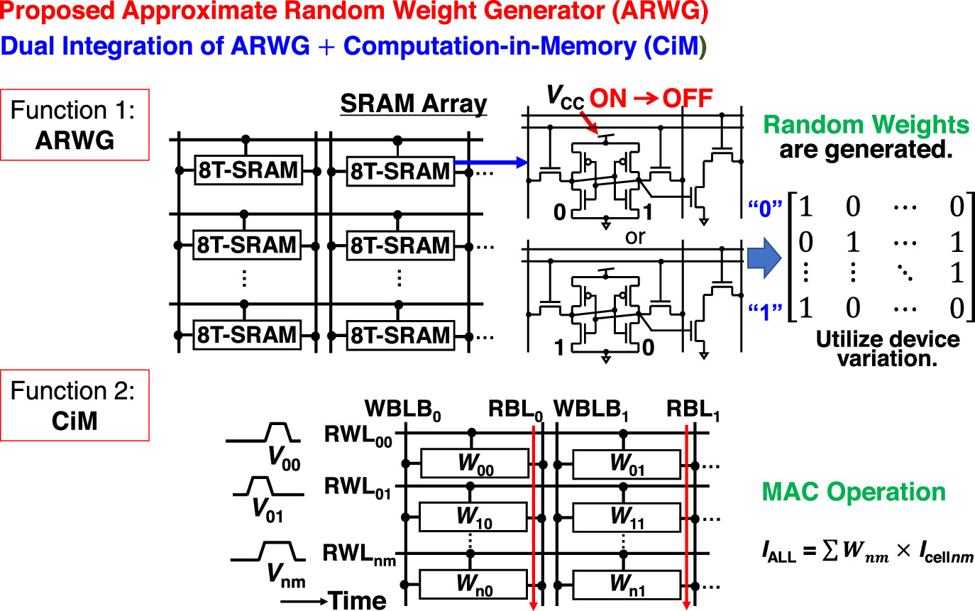
2. Proposed ARWG
Figure 2 shows the proposed ARWG. ARWG integrates generating random weights by utilizing device variation and CiM for MAC operation. The proposed ARWG is composed of 8T-SRAM. Unlike conventional PUFs, the proposed ARWG has a read port. As a result, the proposed ARWG not only generates random weights, but also performs MAC operation. For RC, random weights are used for WIN and WREC, while for random weight SNN random weights are used in the convolution layer. Since random weights are not trained, the proposed ARWG only needs to generate random weights once for 8T-SRAM array (Function 1: ARWG) and uses the generated random weights for MAC operation in both training and inference (Function 2: CiM). As shown in Fig. 3, the conventional circuit configuration consists of RNG for generating random weights and CiM for MAC operation for RC and random weight SNN. In addition, to realize a perfect match, ECC is employed in a controller. However, the proposed ARWG does not require ECC since it does not need to correct weights to make the randomness accurate because RC and random weight SNN allow approximate randomness. Thus, the conventional circuit area is more than twice as large as the proposed ARWG.

Fig. 2. Proposed ARWG.
Download figure:
Standard image High-resolution image
Fig. 3. Circuit area comparison between the conventional circuit configuration and the proposed ARWG for RC and random weight SNN.
Download figure:
Standard image High-resolution imageFigure 4 describes the operation of the proposed ARWG with (a) input events and VCC relative to time and (b) circuit operation in the 8T-SRAM array. There are four phases of the operation. Phase 1 is random weight setting. When VCC starts up, the proposed ARWG generates random weights based on the uniqueness of SRAM device variation. If power is supplied to VCC, an 8T-SRAM generates either "1" or "0" depending on device variation. SRAM device variation makes randomness in the weights of RC or random weight SNN. Phase 2 is MAC operation. Since VCC remains supplied, the random weights generated in Phase 1 are kept stored in the 8T-SRAM array. Therefore, the proposed ARWG can use the random weights for MAC operation. If input events occur, read word-lines become high. The results of MAC operation are obtained by sensing read bit-lines. Phase 3 is random weight resetting. Phase 3 shows when VCC is turned off, such as in cases where users stop using ARWG or change ARWG from training to inference. When power is off in VCC, the random weights used during Phases 1 and 2 cannot be kept stored in the 8T-SRAM array. Phase 4 is random weight setting. Phase 4 indicates how the random weights are restored to perform MAC operation again because ARWG is powered off in Phase 3. Although the random weights are reset in Phase 3, because VCC is turned off the 8T-SRAM requires the random weights to be the same as those during Phases 1 and 2 for MAC operation. In Phase 4, utilizing SRAM device variation, random weights are restored. If power is again supplied to VCC, the 8T-SRAM generates the same weights of "1" or "0" as in Phase 1 because the SRAM device variations are device-specific.

Fig. 4. ARWG operation with (a) input events and VCC and (b) circuit operation in 8T-SRAM.
Download figure:
Standard image High-resolution imageOperation of the proposed ARWG does not imply that device-specific randomness is required for each network but suggests that device-specific randomness can satisfy the random weights in RC and random weight SNN.
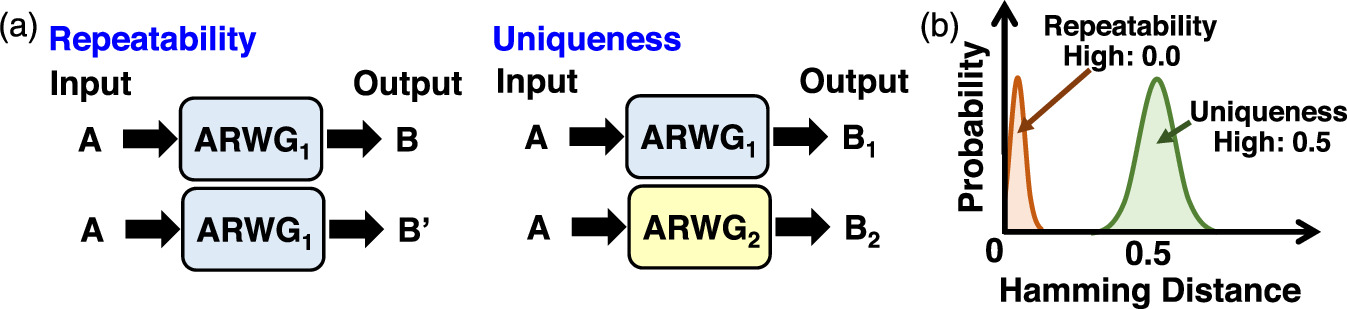
The proposed ARWG is used for RC and random weight SNN. On the other hand, PUFs are used for identification, individual authentication, and security technology. RNGs are used for encryption and security technology. Because they have different uses, their randomness requirements are different. To evaluate randomness compared with PUFs and RNGs, repeatability and uniqueness are defined, as shown in Fig. 5(a). Repeatability is defined as a property that reproduces the same output to the same device. Uniqueness is defined as a property that returns a different output for a given input to the different devices. As shown in Fig. 5(b), when the Hamming distance is close to 0.0, repeatability increases, whereas when the Hamming distance is close to 0.5, uniqueness increases. Table I shows the ideal requirements for repeatability and uniqueness from the intended use of PUFs, RNGs and ARWG. PUFs require high repeatability and do NOT allow errors by providing ECC in the controller. RNGs must not reproduce the same output. For the proposed ARWG, the requirements from the network side of RC and random weight SNN are shown. The requirements can be used as the criteria that the proposed 8T-SRAM ARWG must satisfy in its fabrication. For repeatability, the proposed ARWG allows a Bit-error rate as high as 0.1%. 4,8) The proposed ARWG generates once random weights for the 8T-SRAM array and uses the random weights for MAC operation. Repeatability for the proposed ARWG is considered as the Bit-error rate when random weights generated once in Phase 1 are restored for MAC operation in Phase 4. In other words, random weights with a Bit-error of less than 0.1%, approximate random weights, are allowed when restoring random weights using SRAM device variations. For uniqueness, PUFs and RNGs require high uniqueness, 0.5 of the Hamming distance. For example, according to a paper, 26) the measured HD of the SRAM array is approximately 0.485–0.497. Although SRAM array is used for PUFs and RNGs, the quality of the randomness requires improvement. However, RC and random weight SNN can allow the value of the measured HD, which is revealed in the following section. In the next section, the randomness of random weights generated by the proposed ARWG is analyzed. Although the randomness is focused on in the following sections, it is important to keep in mind that the proposed ARWG is not just a random weight generator but can also perform CiM function.

Fig. 5. Definition of (a) repeatability and uniqueness with (b) Hamming distance.
Download figure:
Standard image High-resolution imageTable I. Comparison between PUF, RNG and the proposed ARWG.
| Physically unclonable function (PUF) | Random number generator (RNG) | Prop. ARWG | |
|---|---|---|---|
| Repeatability | Required w/ECC a) | Must not | Acceptable Bit-error rate |
| < 0.1% [4, 8] | |||
| Uniqueness | Required | Required | Approximate |
3. Randomness of random weight generated by ARWG
In this section, the randomness of random weights generated by the proposed 8T-SRAM ARWG are discussed. Figure 6 shows the circuit configuration of the proposed 8T-SRAM ARWG (a) without a dummy cell and (b) with a dummy cell. While PUFs or RNGs use a 6T-SRAM to generate random numbers, the 6T-SRAM responses are either "1" or "0" due to the difference between the threshold voltages (Vth) of both PMOS transistors. The proposed ARWG has extra 2T-SRAM for MAC operation. Figure 7 shows Monte Carlo simulation results from 0–2 ms with (a) VCC, (b) VQ without a dummy cell and (c) VQ with a dummy cell. To show further details, Figs. 7(d) and 7(e) describe the results from 0–120 μs with (d) VQ without a dummy cell and (e) VQ with a dummy cell. Figure 8 shows the probability of response "1" or "0" from the proposed ARWG with and without a dummy cell. For the proposed ARWG without a dummy cell, the probability of response "1" is higher than response "0". Because QB is connected to N6, QB is subject to N6, and tends to become low. As a result, the probability of response "1" increases. To improve the responses from the proposed ARWG, a dummy cell is applied. Due to the dummy cell, the proposed ARWG improves the probability of the response by 19.2%. Figure 9 shows the probability of responses "1" and "0" from the proposed ARWG without a dummy cell when the width of the read port is changed. The read port consists of N5 and N6 for MAC operation as the function of CiM. If a dummy cell is not used, the capacity of Q is smaller than the capacity of QB. Therefore, the probability of response "1" increases. Increasing the width of the read port increases the capacity of QB. As shown in Fig. 9, it can be said that the probability of response "1" increases as the capacity of QB increases. When the read port is wide, the probability of responses between "1" and "0" become extremely unbalanced. To return highly random responses of "1" and "0", where the probability of response is 0.5, a dummy cell is very useful. Although the read port consists of two transistors, one dummy cell is effective, and thus, the circuit area can be reduced.

Fig. 6. Circuit configuration of the 8T-SRAM ARWG (a) without a dummy cell and (b) with a dummy cell.
Download figure:
Standard image High-resolution image
Fig. 7. Monte Carlo simulation results from 0–2 ms with (a) VCC and (b) VQ without a dummy cell. Monte Carlo simulation results from 0–120 μs with (c) VQ with a dummy cell, (d) VQ without a dummy cell and (e) VQ with a dummy cell.
Download figure:
Standard image High-resolution image
Fig. 8. Probability of response "1" and "0" from the proposed ARWG with and without a dummy cell.
Download figure:
Standard image High-resolution image
Fig. 9. Probability of response "1" and "0" from the proposed ARWG without a dummy cell when the width of the read port is changed.
Download figure:
Standard image High-resolution imageThe randomness of random weights is affected by variation of temperature. Figure 10 shows the probability of responses "1" and "0" from the proposed ARWG with a dummy cell with different temperatures. Although the temperature increases, the probability of response "1" slightly decreases. The difference between the probability of "1" and "0" is within 1.0% randomness of the proposed ARWG, which can be changed due to process variations. Figure 11 shows the probability of responses from the proposed ARWG with a dummy cell with corner variations. In the case of SS, where both pMOS and nMOS are slow, this results in the most unbalanced probability between responses "1" and "0". However, the difference in probability is less than 1.0%. Finally, Fig. 12 shows the Hamming distance calculated from 1000 Monte Carlo simulations assuming an 8×8 8T-SRAM array. The distribution is centered at 0.5, which can be said to be ideal. As discussed above, the proposed 8T-SRAM ARWG improves the randomness of random weights by applying a dummy cell and generates high quality of random weights within 1.0% error.

Fig. 10. Probability of response "1" and "0" from the proposed ARWG with a dummy cell with different temperatures.
Download figure:
Standard image High-resolution image
Fig. 11. Probability of response "1" and "0" from the proposed ARWG with a dummy cell with corner variations.
Download figure:
Standard image High-resolution image
Fig. 12. Hamming distance calculated from 1000 Monte Carlo simulations assuming 8×8 8T-SRAM Array.
Download figure:
Standard image High-resolution image4. Evaluation of randomness required from event-based neuromorphic computing
4.1. Iteration period and Hamming weight for RC and random weight SNN
To evaluate the randomness of random weights for RC and random weight SNN, random weights are generated by specifying the iteration period and Hamming weight. Figure 13 shows examples of random weights where each weight has 3-bit precision generated by specifying (a) the iteration period and (b) Hamming weight. The iteration period is defined as the unit of a pattern. Random weights are generated by repeating the iteration period. To correlate the evaluation from the network side with the proposed 8T-SRAM array, the iteration period is converted to Hamming distance, which is generally used for the evaluation of SRAM chips. Hamming weight is defined as the probability of "1" in the element of a vector. Figure 14 shows the relationship between the Hamming distance and iteration period of (a) 3, (b) 10, (c) 100 and (d) 1000. Figure 15 shows the relationship between the Hamming distance and Hamming weight of (a) 0.01, (b) 0.1, (c) 0.3 and (d) 0.5. The Hamming distance is calculated from two WREC in 1000 trials if reservoir size N = 1000 and there is 3-bit precision for WREC in RC. As the iteration period becomes longer, variance becomes smaller and closer to 0.5 of the Hamming distance, resulting in better uniqueness of random weights. Similarly, as the Hamming weight becomes closer to 0.5, the average value of the Hamming distance becomes closer to 0.5, better uniqueness of random weights. In this study, DVS128 31) Gesture Dataset is employed for the gesture recognition task using RC and random weight SNN. In the gesture recognition task, event-based data are classified into 11 categories such as "arm roll" and "right-hand clockwise." The input size of event-based data during training and inference is 128 (height) × 128 (width) for ON and OFF events, respectively. Note that 80% of recognition accuracy is used as the criterion.

Fig. 13. Random weights generated by specifying (a) the iteration period and (b) Hamming weight.
Download figure:
Standard image High-resolution image
Fig. 14. Relationship between the iteration period and Hamming distance. Frequency at Hamming distance with iteration period of (a) 3, (b) 10, (c) 100 and (d) 1000.
Download figure:
Standard image High-resolution image
Fig. 15. Relationship between the Hamming weight and Hamming distance. Frequency at Hamming distance with Hamming weight of (a) 0.01, (b) 0.1, (c) 0.3 and (d) 0.5.
Download figure:
Standard image High-resolution image4.2. Evaluation of randomness for RC
In RC, the input layer has 162 inputs by leaky integrate-and-fire pooling the event-based data. For the reservoir layer, reservoir sizes of 1000, 500 and 200 are analyzed, respectively. Linear regression is used as the classifier and the output layer has 11 outputs. The reservoir layer and output layer are fully connected and only WOUT between the reservoir layer and output layer is trained. 4) Figure 16 shows the recognition accuracy of RC with different iteration periods (a), (c), (e) in WIN, and (b), (d), (f) in WREC. In evaluating WIN and WREC, the weights of WREC and WIN are set to Gaussian distribution, respectively. Reservoir size N is (a), (b) 1000, (c), (d) 500, and (e), (f) 200. For reservoir size N = 1000 and 500, more than 102 and 103 iteration periods are required for both WIN and WREC, respectively. For reservoir size N = 200, although more than 103 iteration period is required for WIN, it can be said that recognition accuracy with different iteration periods in WREC is unstable. When the iteration period is less than 102 in WIN, recognition accuracy significantly decreases.

Fig. 16. Recognition accuracy with different Iteration periods of RC in (a), (c), and (e) in WIN and (b), (d), and (f) in WREC. Reservoir size N is (a), (b) 1000, (c), (d) 500, and (e), (f) 200.
Download figure:
Standard image High-resolution imageFigure 17 shows the recognition accuracy of RC with different Hamming distances (a), (c), (e) in WIN, and (b), (d), (f) in WREC. Reservoir size N is (a), (b) 1000, (c), (d) 500, and (e), (f) 200. For WIN, acceptable Hamming weights are between 0.1 and 0.9 for reservoir size N of 1000 and between 0.1 and 0.8 for reservoir size N of 500. As the reservoir size decreases to 200, the range of acceptable Hamming weights is smaller, from 0.1–0.7. For WREC, Hamming weight from 0.01–0.99 is acceptable regardless of reservoir size. The results indicate that WIN is more sensitive than WREC.

Fig. 17. Recognition accuracy with different Hamming weight of RC in (a), (c), and (e) in WIN and (b), (d), and (f) in WREC. Reservoir size N is (a), (b) 1000, (c), (d) 500, and (e), (f) 200.
Download figure:
Standard image High-resolution imageFigure 18 shows recognition accuracy with different Hamming weights in both WIN and WREC. If the Hamming weight is extremely small or large, recognition accuracy decreases significantly. When Hamming weights are 0.1 for WIN and between 0.1 and 0.5 for WREC, recognition accuracy is high.

Fig. 18. Recognition accuracy with different Hamming weights in both WIN and WREC.
Download figure:
Standard image High-resolution imageFigure 19 shows extreme examples with reservoir state transitions. Figure 19(a) shows the reservoir state transitions when (a) the Hamming weights of WIN and WREC are 0.5. The random weights of both WIN and WREC are unique. Figure 19(b) shows the reservoir state transitions when WIN is initialized to a positive value and the Hamming weight of WREC is 0.5, while Fig. 19(c) shows when the Hamming weight of WIN is 0.5 and WREC is initialized to a positive value. As shown in Fig. 19(b), almost all reservoir states stick to +1 and are no longer functional. However, Fig. 19(c) shows that the reservoir state transitions properly despite all positive values of WREC. The results indicate that the function of WIN is to transmit input, while WREC is only intended to assist short-term memory.
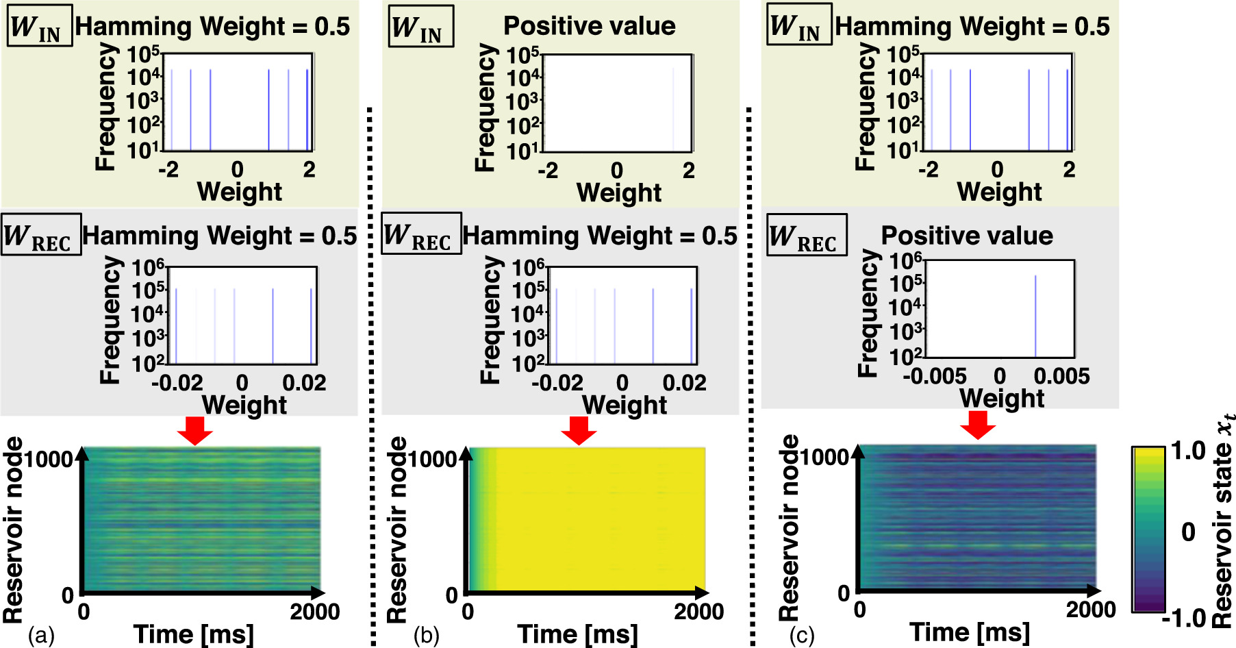
Fig. 19. Extreme examples with reservoir state transitions when (a) the Hamming weights of WIN and WREC are 0.5. (b) WIN is initialized to a positive value while the Hamming weight of WREC is 0.5. (c) Hamming weight of WIN is 0.5 while WREC is initialized to a positive value.
Download figure:
Standard image High-resolution image4.3. Evaluation of randomness for random weight SNN
In random weight SNN, random weights are used in the convolution layer. The size of the convolution layer is 17  17.
8) Under the same conditions as RC, linear regression for the classifier and 11 outputs are used. For random weight SNN, 102 or more Iteration period [Fig. 20(a)] and Hamming weight between 0.01 to 0.9 [Fig. 20(b)] are required in convolutional weights. Compared with RC, both the iteration period and Hamming weight of random weight SNN have similar trends to WIN of RC.
17.
8) Under the same conditions as RC, linear regression for the classifier and 11 outputs are used. For random weight SNN, 102 or more Iteration period [Fig. 20(a)] and Hamming weight between 0.01 to 0.9 [Fig. 20(b)] are required in convolutional weights. Compared with RC, both the iteration period and Hamming weight of random weight SNN have similar trends to WIN of RC.

Fig. 20. Recognition accuracy with different (a) iteration periods and (b) Hamming weights.
Download figure:
Standard image High-resolution image
As a result, the randomness required for RC and random weight SNN is significantly lower than that of PUFs and RNGs. This means that approximate random weights are allowed for RC and random weight SNN.
Table II. Summary of this study.
| ARWG for reservoir computing | |||||||||
|---|---|---|---|---|---|---|---|---|---|
| Reservoir size N = 200 | Reservoir size N = 500 | Reservoir size N = 1000 | ARWG for random weight SNN | ||||||
| W IN | W REC | W IN | W REC | W IN | W REC | PUF | RNG | ||
| Uniqueness (HD) | 0.45 < HD < 0.55 | — | 0.45 < HD < 0.55 | 0.45 < HD < 0.55 | 0.3 < HD < 0.7 | 0.3 < HD < 0.7 | 0.3 < HD < 0.7 | 0.5 | — |
| Hamming weight (HW) | 0.1 < HW < 0.7 | 0.01 < HW < 0.99 | 0.1 < HW < 0.8 | 0.01 < HW < 0.99 | 0.1 < HW < 0.9 | 0.01 < HW < 0.99 | 0.01 < HW < 0.9 | 0.5 | 0.5 |
5. Conclusion
In this paper, dual integration design of ARWG and CiM is proposed for event-based RC and random weight SNN. This paper discusses the functions and circuit operation of the proposed ARWG, and the randomness of the random weights generated by the proposed ARWG. For the circuit design of the proposed ARWG, a dummy cell is proposed in order to improve the probability of response "1" or "0" for generating random weights. With this proposed dummy cell, the probability of response "1" or "0" has an error of less than 1.0% of the ideal value of 0.5. Table II shows a comparison of the randomness with Hamming distance and Hamming weight for ARWG, PUFs and RNGs. For uniqueness, a Hamming distance between 0.3 and 0.7 is accepted for ARWG in the case of RC (N = 1000) and random weight SNN, while the Hamming distance for PUFs must be 0.5. For Hamming weight, although 0.5 is required for PUFs and RNGs, ARWG for RC and random weight SNN accepts Hamming weight between 0.01 and 0.99 and Hamming weight between 0.01 and 0.9, respectively. Because low randomness is allowed for RC and random weight SNN, the proposed dual integration of ARWG and CiM can facilitate event-based RC and random weight SNN training by generating approximate random weights and performing CiM operations.
Acknowledgments
This study was supported by JST CREST, Japan (Grant No. JPMJCR20C3).