


Abstract
Estimating smallholder crop yields robustly and timely is crucial for improving agronomic practices, determining yield gaps, guiding investment, and policymaking to ensure food security. However, there is poor estimation of yield for most smallholders due to lack of technology, and field scale data, particularly in Egypt. Automated machine learning (AutoML) can be used to automate the machine learning workflow, including automatic training and optimization of multiple models within a user-specified time frame, but it has less attention so far. Here, we combined extensive field survey yield across wheat cultivated area in Egypt with diverse dataset of remote sensing, soil, and weather to predict field-level wheat yield using 22 Ml models in AutoML. The models showed robust accuracies for yield predictions, recording Willmott degree of agreement, (d > 0.80) with higher accuracy when super learner (stacked ensemble) was used (R2 = 0.51, d = 0.82). The trained AutoML was deployed to predict yield using remote sensing (RS) vegetative indices (VIs), demonstrating a good correlation with actual yield (R2 = 0.7). This is very important since it is considered a low-cost tool and could be used to explore early yield predictions. Since climate change has negative impacts on agricultural production and food security with some uncertainties, AutoML was deployed to predict wheat yield under recent climate scenarios from the Coupled Model Intercomparison Project Phase 6 (CMIP6). These scenarios included single downscaled General Circulation Model (GCM) as CanESM5 and two shared socioeconomic pathways (SSPs) as SSP2-4.5and SSP5-8.5during the mid-term period (2050). The stacked ensemble model displayed declines in yield of 21% and 5% under SSP5-8.5 and SSP2-4.5 respectively during mid-century, with higher uncertainty under the highest emission scenario (SSP5-8.5). The developed approach could be used as a rapid, accurate and low-cost method to predict yield for stakeholder farms all over the world where ground data is scarce.
Export citation and abstract BibTeX RIS

Original content from this work may be used under the terms of the Creative Commons Attribution 4.0 licence. Any further distribution of this work must maintain attribution to the author(s) and the title of the work, journal citation and DOI.
1. Introduction
Smallholder farms are increasing around the world, particularly in arid and semi-arid regions, despite regular natural disasters and food insecurity [1, 2]. Accurate and timely estimation of smallholder production is crucial for agronomic management optimization, investment guidance, yield gap analyses, and policy formulation to improve food security [3, 4]. Furthermore, climate change [5], management practices, and land fragmentation all contribute to considerable heterogeneity in yield productivity by smallholders in arid and semi-arid areas [6]. Yield estimates necessitate massive ground observations and specialized technologies, yet field scale yield and weather observations are sometimes unavailable, making smallholder yield assessment a challenge.
Satellite remote sensing (RS) can be utilized to estimate smallholder yield in a fast and low-cost approach on a spatial explicit system [7–10]. RS can be used in crop type mapping and estimating yield using various vegetative indices (VIs) [11–13]. Among these indices are normalized difference vegetation index (NDVI), and enhanced vegetation index (EVI), both of which are widely used [14–16]. However, the applicability of using NDVI and EVI to estimate crop yield has some limitations due to their dependence on crop types and region conditions, requiring the development of other indices such as green chlorophyll vegetation index (GCVI), wide dynamic range vegetation index (WDRVI), and Green Normalized Difference Vegetation Index (GNDVI) [17–20]. In the current study, we used all five VIs, NDVI, EVI, GCVI, WDRVI, and GNDVI, to estimate wheat crop yield with low constraints.
However, relying solely on VIs to estimate yield is insufficient because they do not consider the effects of environmental stresses on crop growth and development [21, 22]. This emphasizes the significance of incorporating other variables such as climate, soil qualities, and terrain. Weather variables such as air temperature and rainfall are commonly utilized to predict agricultural productivity [23]. Because of the relevance of gridded weather data as crucial inputs for yield prediction systems, the use of direct weather data has lately spread [24, 25]. Furthermore, climate change has a negative impact on crop production [26], necessitating ongoing research to investigate these impacts and create viable solutions. Thus, considering weather data variables in yield prediction systems is not only important for current yield predictions, but also in the future predictions. Because of the complex relationships between soil properties and crop yield [27], soil properties are also important variables in crop yield predictions [28], necessitating the best understanding of landscape and soil property variability and their effect on crop yield, which is a critical component of site-specific and sustainable management systems [29, 30]. Topography is considered one of the most important factors affecting crop yield [31], yet it has less attention so far to be used in crop yield predictions at scale. Elevation, slope, and aspect are topography factors that are important for characterizing spatial heterogeneity and the abiotic environment in a given region [32]. Nevertheless, integrating these multivariate variables of RS, climate data, soil properties and topography in a fusion approach to predict crop yield at scale has less attention so far, confirming the importance of the current study to develop this approach to predict wheat yield spatially in Egypt.
Yield prediction is often done dynamically using crop models [33–35], or statistically using statistical regression models [36, 37], depending on the dataset availability and user knowledge. Crop models are powerful tools in predicting yield and attributed physiological processes of crop growth and development under different Genotype (G) × Environment (E), and Management (M) [38–40]. Crop models, on the other hand, require high-quality inputs such as soil, weather, management practices, genetics, and costly computations [41], restricting their application in yield prediction at scale and presenting uncertainties [42, 43]. Furthermore, crop models have restricted inputs, and integrating extra variables such as remote sensing indices and geographic characteristics necessitated subroutine development, which might take a long time [44]. Machine learning (ML) uses training and testing methods to estimate crop production based on crop yield and region characteristics (i.e., RS, climate, soil, and topography), demonstrating their ability to include broad and diverse dataset [45, 46]. ML often beats traditional linear regression because it can separate the effects of co-linear factors and examine hierarchical and nonlinear interactions between predictors and target variables [47, 48]. Furthermore, ML offers additional benefits such as, but not limited to, decreased computation requirements, working simply and quickly in big data at spatial explicit routine, explore the important features (predictors), and the ability to include different variables influencing the response variable [49]. Thus, AutoML could be used as a fast, robust and cheaper tool to help decision makers with yield predictions at scale. There are different ML models which could be used in crop yield predictions such as Neural Networks [50], clustering, random forest and support vector machines [51, 52], and deep learning [53].
Integrating several ML models is crucial in applications to enhance prediction and minimize uncertainty, requiring an integrated library for rapidly and robustly using numerous ML models. Previously, the development of traditional ML focused on design procedure of ML models (i.e., feature engineering, model selection, algorithm selection, hyperparameter tuning, etc), which are time-consuming and cannot be easily redesigned by non-experts [54]. To this end, several AutoML frameworks include Auto-Sklearn [55], tree-based pipeline optimization tool [56], Genetic automated machine learning assistant [57], AutoGluon [58], and H2O AutoML [59] has been proposed to automatically compare and deploying high-performance ML models. These AutoML frameworks have been applied in various disciplines including the estimation of crash severity [60], classification [61], and epidemiology predictions [62]. Nevertheless, AutoML has not been tested in yield predictions based different data sources of remote sensing, field surveys, soil grids and weather conditions, emphasizing the current study novelty. Creating straightforward, uniform interfaces to a range of machine learning algorithms was one of the first steps towards simplification of machine learning (e.g. H2O) [63]. H2O's AutoML can be used to automate the machine learning workflow, which includes automatic model training and tuning within a user-specified time constraint [64], outperforming the traditional ML techniques. Because of the importance of employing a stacked ensemble model (a combination of several machine learning models) in improving predictions, H2O's AutoML can prepare it automatically in a limited number of scripts code and in a straightforward manner. Nonetheless, this library was newly launched and has received less attention in agricultural systems and crop yield estimates thus far. Furthermore, integrating various predictors such as RS, soil properties, topography, and weather data into ML to predict crop yield at scale still need much attention, particularly in arid and semi arid regions.
Therefore, the overall objective of this work is to develop a fusion approach in H2O's AutoML that combines various variables of RS, soil, weather, and topography dataset to predict wheat yield at scale in Egypt (area of interest). To achieve such goal, different objectives were considered and included: (I) collection of ground truth points of winter crops and farmer wheat yield; (II) crop type mapping using ground truth points, and random forest classification; (III) developing fusion approach of yield predictions at spatial explicit manner; and (IV) determining wheat yield based on RS indices and climate change scenarios.
2. Materials and methods
2.1. Study region
Egypt is the area of interest (figure 1) as it is the largest wheat importer country worldwide, its strategic location between three continents (Africa, Asia, and Europe), its rapid population growth, land fragmentations, and its arid climate. The geographical boundary of Egypt is latitude 22°–32° N and longitude 25°–35° E (figure 1). Wheat is the dominant winter crop in Egypt, and the total cultivation area of wheat is around 1.5 M ha. In general, Egypt's climate is dry and hot in summer (April-September) and somewhat damp and cold in winter (October to March) [65]. Temperature increases from North to South of Egypt and the average increase of mean temperature reaches about 3 °C–5 °C during wheat growing season (November—April) [25].

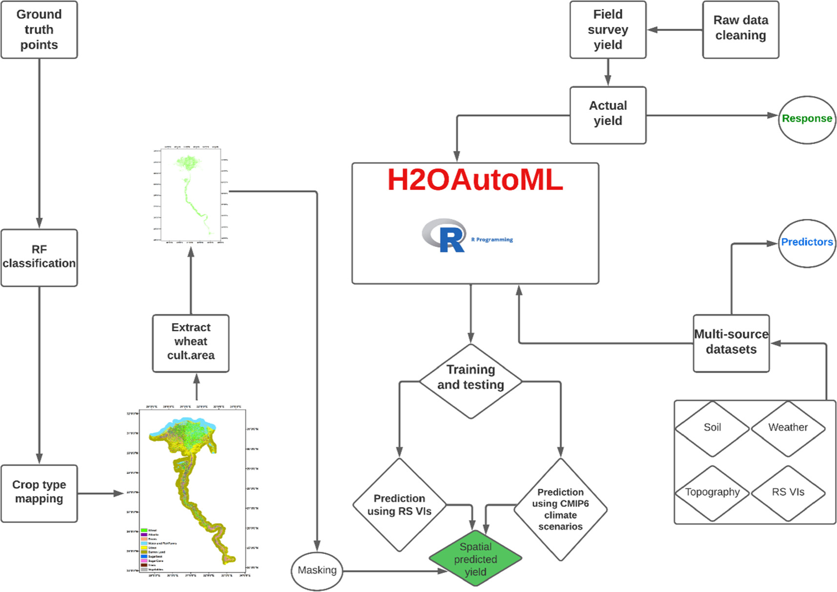
Figure 1. The analytical framework of the developed approach to achieve the study objectives. Ground truth points of winter crops during three successive growing seasons (2019/2020, 2020/2021, and 2021/2022) were used in random forest classifier for producing crop type mapping in Google Earth Engine. The wheat cultivated area was extracted from these maps and used as a mask of the spatial predicted yield. The developed H2OAutoML approach was trained and tested using a fusion of multiple dataset such as soil grid, ERA5 weather data, topography (i.e., elevation (S. Figure 1), aspect, and slope), and remote sensing vegetation indices which are used as predictors. The actual wheat yield collected by many survey rounds was used as a target variable (response) to train and test the ML approach. The default testing by dividing the entire data set into 80% training and 20% testing using a random selection approach was used in training and testing the dataset. Following the training, the validated models were deployed for unseen predictions of wheat yield using two approaches, the first approach is to predict wheat yield using RS vegetative indices; and the second approach is to predict wheat yield using CMIP6 climate scenarios in the mid term (2050).
Download figure:
Standard image High-resolution image2.2. Data processing
Different geospatial datasets were collected and included vegetation indices (Eq1-Eq5), topography, soil properties, weather dataset, and field survey data. Five RS indices such as Normalized Difference Vegetation Index (NDVI), Enhanced Vegetation Index (EVI), green chlorophyll vegetation index (GCVI), Green Normalized Difference Vegetation Index (GNDVI), and Wide Dynamic Range Vegetation Index (WDRVI) were processed and downloaded in monthly time steps using Terra Vegetation Indices 16-Day Global at 250 m resolution from Google Earth Engine (GEE). Other static variables as topography (elevation, aspect, and slope), as well as soil properties (i.e., sand, silt, clay, soil organic carbon, pH, and bulk density) were also downloaded by MODIS at 250 m resolution and calibrated using observed dataset in two locations. To match the yield data in Egypt, we aggregated such indices to the field level. Such processes were implemented in Google Earth Engine (GEE). Monthly weather data such as maximum temperature, minimum temperature, solar radiation, and precipitation were collected from The ERA5 global reanalysis at 31 km resolution [66]. Meanwhile, CMIP6 climate scenarios include one General Circulation Model (GCM) as CanESM5 and two shared socioeconomic pathways (SSPs) as SSP2-4.5 and SSP5-8.5 during the mid-term period (2050) were extracted from recent downscaled data by [67]. To align with the response variable (yield) of refined 2000 yield survey locations, we extracted the geospatial dataset of RS, soil, and weather for the same yield sites from the area of interest's raster dataset (Egypt). Analysis and description of all yield data and secondary dataset are presented in S. Table 1.


Where, NIR is the near-infrared band, R is the red band, G is the green band, and B is the blue band.
2.2.1. Field survey wheat yield
The Agricultural Research Center in Egypt (ARC) employed agricultural specialists and agronomists to evaluate yields in over 2500 fields annually through 2020/2021 and 2022/2023 growing seasons2, covering the Nile valley and Delta. The experts took five 3 × 3 m2 plots diagonally, one from each of the field's four corners and its center, at random from each field. Three measurement replications were used to examine the 1000-grain weight and quantity of kernels in 20 typical ears within the sample plot. The following equation was used for the final yield estimation:

Where Y is the final yield (kg ha−1), EN is the number of ears, KS is the number of kernels per spike, and GW is the 1000-grain weight. To ensure that the yield is totally dry without moisture, the product was multiplied by factor 0.85. For the growing season 2021/2022, farmers' field surveys were deployed by ICARDA using a structured questionnaire with fields geotagged from the particular plot. Data cleaning processes were done on the raw data to remove any outliers. The detailed outputs of wheat yield which includes different cultivars and planting dates were presented in figure 2.

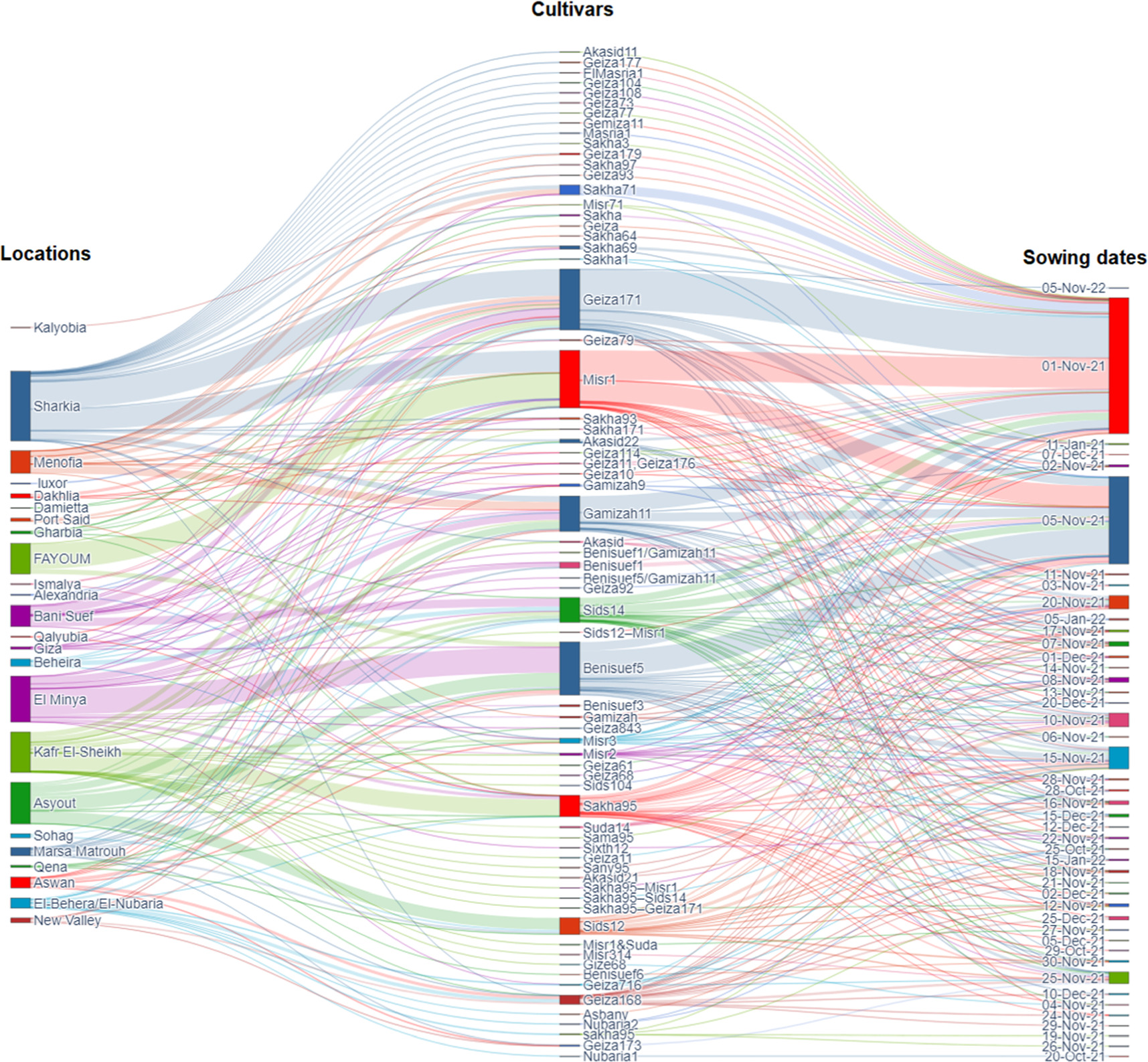
Figure 2. The Sankey diagram shows the actual yield from farmers subjected to different cultivars and sowing dates. About 60 cultivars and 40 sowing dates were used in the analysis.
Download figure:
Standard image High-resolution image2.2.2. Wheat cultivated area
Ground truth points of wheat and other winter crops were collected over three growing seasons (2020, 2021, and 2022) for preparing crop type mapping. Random Forest classification machine learning model was used to train and test these points by Sentinel 2 [68] at 10 m resolution in GEE using free cloud images (https://github.com/DrAhmedKheir/CropTypeMapping.git) . Supplementary figure 2 represent crop type mapping in Egypt for three winter growing seasons, 2020,2021, and 2022 with accuracy 0.912, 0.90, and 0.913 respectively. From these maps, wheat cultivated area was extracted (figure 1), and used as a mask for the estimated yield.
2.3. H2O AutoML
The open source, scalable, networked machine learning framework H2O has a completely automatic supervised learning method called H2O AutoML. In addition to a web GUI, H2O AutoML is also accessible in Python, R, Java, and Scala. The technique is entirely automated, but many of the settings are made available to the user as parameters so that some parts of the modelling phases can be changed. In our case, we developed H2OAutoML in R language and the full script is hosted on GitHub at https://github.com/DrAhmedKheir/H2O_AutoML.git.
2.3.1. Dataset preprocessing and AutoML training
Currently, all H2O supervised learning algorithms offer the same kind of automatic data-preprocessing as H2O AutoML. Categorical data can be handled natively because H2O tree-based models (Gradient Boosting Machines, Random Forests) provide group-splits on categorical variables. Although it is not yet included in the most recent stable release (H2O v3.30.0.3), there are benchmarked several automatic target encoding strategies for high cardinality features in experimental versions of the algorithm. The H2O AutoML roadmap includes additional data pre-processing procedures like automatic text encoding using Word2Vec, feature selection, and feature extraction for automatic dimensionality reduction [63]. The AutoML techniques can assist in designing the optimal ML models in a constrained amount of time by automatically choosing ML models and stack ensembles based on various algorithms and training strategies [54]. With just one function, the H2O AutoML offers a distributed ML learning platform that can quickly and thoroughly automate the training of candidate models and stacked ensembles. A scoreboard based on a variety of model performance indicators, training duration, or average prediction speed will list all candidate models. Fast random search and stacked ensembles are combined in H2O AutoML to train many algorithms, including deep neural networks, random forests, XGBoost gradient boosting machines (GBM), and generalized linear models.
2.3.2. Models
H2O AutoML includes base models and Stacked Ensembles. The base models include XGBoost Gradient Boosting Machines (GBM), Gradient Boosting Machines (GBM), Random Forests10 (Default and Extremely Randomized Tree variety), Deep Neural Networks and Generalized Linear Models (GLM), allowing GPU acceleration of training. If the base models are each strong and have uncorrelated errors, stacked ensembles, or super learners, perform especially well. A very diversified set of base models are produced via random search across numerous algorithm families, and when stacking is added, powerful ensembles are created. Here, we chose 20 models in H2O AutoML, and the outputs comprised 22 models, implying that two stacked ensembles were created, one for all models and another for the best of all models. Table 1 displays the names and accuracy of these models.
Table 1. List of models and related accuracies from H2O AutoML ordered from higher accuracy [1] to lower accuracy [22].
| No | Model_id | RMSE | MSE | MAE | RMSLE | MRD |
|---|---|---|---|---|---|---|
| 1 | StackedEnsemble_AllModels_1_AutoML | 1.225725 | 1.502401 | 0.902811 | 0.198735 | 1.502401 |
| 2 | StackedEnsemble_BestOfFamily_1_AutoML | 1.229863 | 1.512562 | 0.905335 | 0.19929 | 1.512562 |
| 3 | GBM_4_AutoML | 1.237023 | 1.530225 | 0.907529 | 0.19986 | 1.530225 |
| 4 | GBM_5_AutoML | 1.237726 | 1.531965 | 0.915031 | 0.201057 | 1.531965 |
| 5 | GBM_2_AutoML | 1.240838 | 1.53968 | 0.912857 | 0.201092 | 1.53968 |
| 6 | XRT_1_AutoML | 1.243359 | 1.545941 | 0.90307 | 0.200125 | 1.545941 |
| 7 | GBM_3_AutoML | 1.244005 | 1.547549 | 0.914904 | 0.201274 | 1.547549 |
| 8 | GBM_grid_1_AutoML | 1.245269 | 1.550696 | 0.910393 | 0.199793 | 1.550696 |
| 9 | DRF_1_AutoM | 1.246086 | 1.552732 | 0.903185 | 0.20058 | 1.552732 |
| 10 | GBM_grid_1_AutoML | 1.250137 | 1.562842 | 0.919526 | 0.202063 | 1.562842 |
| 11 | GBM_grid_1_AutoML | 1.254352 | 1.573398 | 0.932354 | 0.203407 | 1.573398 |
| 12 | GBM_grid_1_AutoML | 1.264679 | 1.599413 | 0.941779 | 0.205372 | 1.599413 |
| 13 | GBM_grid_1_AutoML | 1.264712 | 1.599497 | 0.941486 | 0.206597 | 1.599497 |
| 14 | GBM_1_AutoML | 1.324547 | 1.754425 | 1.008931 | 0.217644 | 1.754425 |
| 15 | DeepLearning_grid_2_AutoML | 1.457579 | 2.124536 | 1.094931 | 0.240186 | 2.124536 |
| 16 | DeepLearning_grid_2_AutoML | 1.480585 | 2.192131 | 1.113768 | 0.246797 | 2.192131 |
| 17 | DeepLearning_grid_3_AutoML | 1.484668 | 2.204238 | 1.09328 | 0.244963 | 2.204238 |
| 18 | GLM_1_AutoML | 1.492311 | 2.226993 | 1.170025 | 0.245378 | 2.226993 |
| 19 | DeepLearning_grid_1_AutoML | 1.522751 | 2.31877 | 1.16936 | 0.248795 | 2.31877 |
| 20 | DeepLearning_grid_3_AutoML | 1.531571 | 2.34571 | 1.18382 | 0.254437 | 2.34571 |
| 21 | DeepLearning_1_AutoML | 1.562223 | 2.440539 | 1.195309 | 0.254975 | 2.440539 |
| 22 | DeepLearning_grid_1_AutoML | 1.58321 | 2.506554 | 1.190176 | 0.262548 | 2.506554 |
RMSE: Root Mean Square Error; MSE: Mean Square Error; MAE: Mean Absolute Error; RMSLE: Root Mean Squared Log Error; MRD: Mean Residual Deviance
2.3.3. Random grid search parameters
To offer the optimal model, AutoML conducts a hyperparameter search over a range of H2O algorithms. The hyperparameters and all possible values that could be selected at random for the search are listed in Supplementary table 2. It's interesting to note that AutoML does not perform a conventional grid search for GLM that returns all potential models. As an alternative, AutoML creates a single model while enabling lambda_search and passing a list of alpha values. Instead of returning one model for each alpha-lambda combination, it just returns the model with the best alpha-lambda combination.
2.4. Performance assessment of the best models
In addition to previous indicators used in H2O AutoML (table 1), we introduced other statistical indicators to assess the model performance. These indicators included determination coefficient (R2), relative bias (RB), root mean square deviation (RMSD) [69], and Willmott degree of agreement (d) [70]. Detailed description of calculating each parameter are presented by [36]. The indicator R2 provides a measure of how well the independent variable(s) in the model explain the variability in the dependent variable. The R-squared value ranges from 0 to 1, with 0 indicating that the model does not explain any variability in the dependent variable, and 1 indicating that the model perfectly explains all the variability. Relative Bias is a normalized measure that expresses the bias as a percentage of the true values. It is particularly useful when comparing models or assessing the accuracy of predictions in different contexts. Relative Bias is calculated by summing the differences between predicted and observed values, dividing by the sum of true values, and then multiplying by 100 to express the result as a percentage. A Relative Bias of 0% indicates no bias, positive values indicate overestimation bias, and negative values indicate underestimation bias. RMSD is particularly useful when you want to penalize larger errors more heavily than smaller errors. Smaller RMSD values indicate better agreement between predicted and observed values. However, like any metric, it should be interpreted alongside other relevant metrics to obtain a comprehensive understanding of model performance. The Willmott Degree of Agreement ranges from 0 to 1, with 1 indicating perfect agreement between the observed and modeled values. A higher value of (d) suggests better agreement and robust model accuracy.
3. Results
3.1. Actual wheat yield and secondary dataset
The dataset from the field survey included 60 local wheat cultivars and 40 sowing windows to ensuring a large number of sites covering all agroclimatic zones in Egypt. The Sankey diagram represented the complex interrelationships between locations, cultivars, and sowing dates (figure 2). Geiza171, Sakha95, Beniseuf5, Misr1, and Gamizah11 were the highest yielding cultivars (figure 2). Furthermore, using a wide range of sowing windows [40], it was found that sowing wheat on the first and/or fifth of November had the maximum yield (7.5–10 t ha−1). Respecting to the highest yield cultivars and their relationships with most related locations and best sowing dates, analysis showed that the cultivar Geiza171 is common in East delta and upper Egypt (Sharkia and Bani-Suef) while the best sowing date windows ranging 01–05 November. The cultivar Sakha95 is very common in Nile delta with broad range of sowing dates (10 November—10 December). This is a high yielding and recent cultivar introduced recently to Egyptian local cultivars with high resistance to rust and salinity stress. There is also another high yielding cultivar in Nile Delta called Gamizah11 with dominant sowing dates from 01 November to 20 November. Moving from high latitude (low temperature) to high latitude (high temperature, South of Egypt), the cultivar Beniseuf5 is very common in such conditions and the best sowing dates are from 01 November to 15 November. Considering all conditions in Egypt, the cultivar Misr1 showed superiority in either North or South of Egypt while the best sowing dates are from 01–05 November.
In terms of secondary datasets such as soil parameters, topography, RS indices, and meteorological data and their associations with actual yield, data in figure 3, S. Figure 3, and S. Figure 4 revealed a variety of relationships. During the wheat growing seasons (November—April), the probability density differed between investigated vegetative indices (supplementary figure 3). The highest values and densities of NDVI, EVI, GCVI, GNDVI, and WDRVI were 0.8, 0.6, 10, 0.8 and −0.2 respectively. For all indices, the maximum peak was noticed during the months January—March. Different soil properties were considered include soil bulk density (BD), clay percentage, and organic matter content (OM). Soil showed heterogeneity from North to South, but the probability densities showed that the highest values and probability densities of BD, clay and OM were 1.5 Mg m−3, 30%–40%, and 0%–2% respectively. Since maximum and minimum temperatures are critical variables in determining crop yield, analysis showed that growing season maximum temperature ranged from 22 °C–26 °C, while minimum temperature ranged from 11 °C–13 °C (supplementary figure 3). Correlation analysis showed that there were positive correlations between clay content in soil, soil organic matter, and RS indices (NDVI, EVI, GCVI, GNDVI, and WDRVI) with actual yield. Meanwhile, the yield correlated negatively with weather data (maximum and minimum temperatures, and solar radiation), elevation and soil bulk density. This confirms the importance of data diversity and heterogeneity to be used in yield predictions.

Figure 3. Correlation plot between different variables of vegetation, topography, soil, weather, and yield. TminAvg (average minimum temperature), DEM (elevation), TmaxAvg (average maximum temperature), SRADAvg (solar radiation), OM (soil organic matter), BD (soil bulk density), and RainAvg (rainfall). Weather and RS indices averaged over growing season of wheat (November to April).
Download figure:
Standard image High-resolution image3.2. Regression analysis between RS indices and actual yield
Remote sensing indices showed weak correlation with yield though the overall relationship is positive (figure 4). Yield increased with increasing vegetative indices recording R2 = 0.035, 0.022, 0.025, 0.022, and 0.022 for NDVI, EVI, GCVI, GNDVI and WDRVI respectively with significant effect (P < 0.001). The weak correlation may be attributed to considering the monthly average value of each index, rather than considering the maximum peak value for each index. Nonetheless, linear regression is a straightforward method that was not considered enough for predicting yield from vegetative indices, opening the way to various non-linear machine learning approaches capable of disentangling the non-linear correlations between VIs and yield. There are other reasons for the weak relationship between vegetative indices and yield using linear regression. Aside from vegetative indicators, a variety of factors influence yield, including environmental conditions (i.e., temperature, rainfall, humidity), soil quality, insect and disease pressure, management strategies (fertilization, irrigation), and genotype. If these parameters are not considered or fluctuate greatly, the correlation between vegetative indices and yield may be weakened. Furthermore, remote sensing data can be spatially and temporally variable, which means that the conditions viewed by the satellite or sensor may not exactly match those on the ground at the time of data collection. This unpredictability may contribute noise into the link between vegetative indices and yield, weakening the correlation. The relationship between vegetative indicators and yield might not be strictly linear. While simple linear regression assumes a linear relationship, the actual relationship between these variables may be non-linear or have diminishing returns. In such circumstances, a more complicated regression model or nonlinear modeling techniques may be required to accurately capture the link. Accordingly, we can notice here in the trained ML improved the accuracy of predicting yield from vegetative indices since it is more sophisticated and considered nonlinear relationships, avoided the weakness of simple linear regression.

Figure 4. Regression analysis between different remote sensing indices such as NDVA (a), EVI (b), GCVI (c), GNDVI (d), and WDRVI ( e) with actual yield.
Download figure:
Standard image High-resolution image3.3. Training and testing H2OAutoML
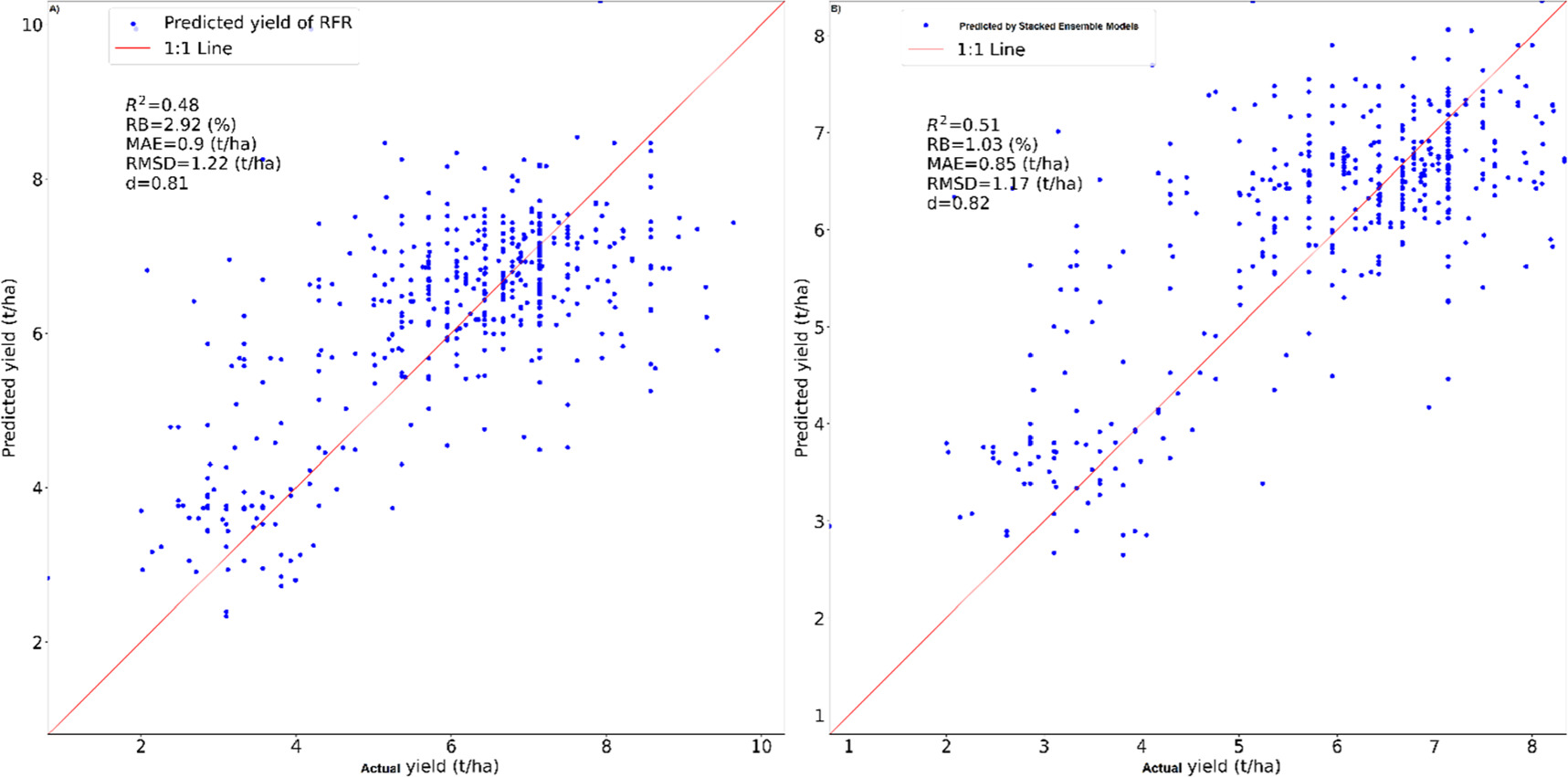
A huge number of candidate models are trained automatically by H2O's AutoML. H2O's AutoML can also be a useful tool for advanced users because it offers a straightforward wrapper function that executes many modeling-related tasks that ordinarily require many lines of code, freeing up their time to concentrate on other data science pipeline tasks like feature engineering, model deployment, and data preprocessing. Here we integrated diverse dataset of soil, weather, RS indices, and topography as predictors while yield represented the response to train and test 20 models in H2O's AutoML. The automatic training and testing in H2O's AutoML, resulted in obtaining 22 models, 20 models as potential models for the current dataset, in addition to two stacked ensemble models (best of family and all models), (table 1). Figure 5 shows the performance of training two models, random forest, and stacked ensemble (best of family). Although, all models (22 models, table 1) showed high accuracy, the stacked ensemble outperformed other models include RF and deep learning models. The stacked ensemble (all models) outperformed all other models, including GBM, XRT, GBM grid, Random Forest (DRF), and deep learning (table 1). The stacked ensemble (all models) had lower values for RMSE, MSE, MAE, RMSLE, and MRD: 1.22, 1.5, 0.9, 0.19, and 1.5, respectively. Such values rapidly grew as other models recorded 1.5, 2.5, 1.19, 0.26, and 2.5 using deep learning models. Considering multi-indices is important to specify the perfect model accuracy, however we included other statistical indicators which are more common in model performance evaluation such as R2, RB, RMSD, and d. The additional indices were used to compare the accuracy of the stacked ensemble model (all models) with another standard and widely used model such as Random Forest (figure 5). Such metrics indicated that RFR predicted the yield robustly recording 0.48, 2.92%, 0.9 t ha−1, 1.22 t ha−1, and 0.81 for the indices R2, RB, MAE, RMSD, and d respectively (figure 5(A)). Such values improved to 0.51, 1.03%, 0.85 t ha−1, 1.17 t ha−1, and 0.82 when the stacked ensemble model was considered (figure 5(B)). This confirms the robust accuracy of the stacked ensemble, and the potential of its deployment in yield predictions using diverse dataset. One of the best advantages of ML, is to explore the important features contributing significantly to determining the response factor (yield). SHAP plot (figure 6) summarized the important features from all datasets used in a sequence order. The important features determined the yield were elevation, sand, rainfall, solar radiation, EVI at first month of growing, maximum temperature, EVI at the fourth month, averaged EVI over the growing season, silt, EVI at the third month, minimum temperature, bulk density, EVI at the second month, clay, soil organic matter, GNDVI at the first month, GCVI at the second month, GNDVI at fifth month, averaged GNDVI over the season, and WDRVI at the fourth month. Interestingly, EVI and GNDVI outperformed other RS indices in determining yield in the study region. Overall, the Wilmott degree of agreement (d) is greater than 80%, demonstrating the robustness of the models' training and their potential for future predictions.

Figure 5. Actual versus predicted yield by Random Forest (A) and by Ensemble of 20 Ml models, best estimator (B) using H2OAutoML routine.
Download figure:
Standard image High-resolution image
Figure 6. Feature importance for grain yield (t ha−1) based on SHAP-values for the Random Forest regression model. The local explanation summary on the right illustrates the relationship between a feature and the model output in terms of direction. While negative SHAP-values indicate a decrease in grain yield, positive SHAP-values indicate an increase in grain yield. The features are elevation (dem), sand, rainfall averaged over the six months from sowing to harvest (RainAvg), solar radiation averaged over the six months from sowing to harvest (SRADAvg), Enhanced Vegetation Index at the first month (EVIM1), maximum temperature averaged over the six months from sowing to harvest (TmaxAvg), Enhanced Vegetation Index at the fourth month (EVIM4), Enhanced Vegetation Index averaged over the six months from sowing to harvest (MeanEVI), silt content in soil (silt), Enhanced Vegetation Index at the third month (EVIM3), minimum temperature averaged over the six months from sowing to harvest (TminAvg), soil bulk density (BD), Enhanced Vegetation Index at the second month (EVIM2), clay content in soil (clay), soil organic matter (OM), Green Normalized Difference Vegetation Index at the first month (GNDVIM1), green chlorophyll vegetation index during the second month (GCVIM2), Green Normalized Difference Vegetation Index at the fifth month (GNDVIM5), Green Normalized Difference Vegetation Index averaged over the six months from sowing to harvest (MeanGNDVI), and the Wide Dynamic Range Vegetation Index over the fourth month (WDRVIM4).
Download figure:
Standard image High-resolution image3.4. Prediction of wheat yield by AutoML using RS indices
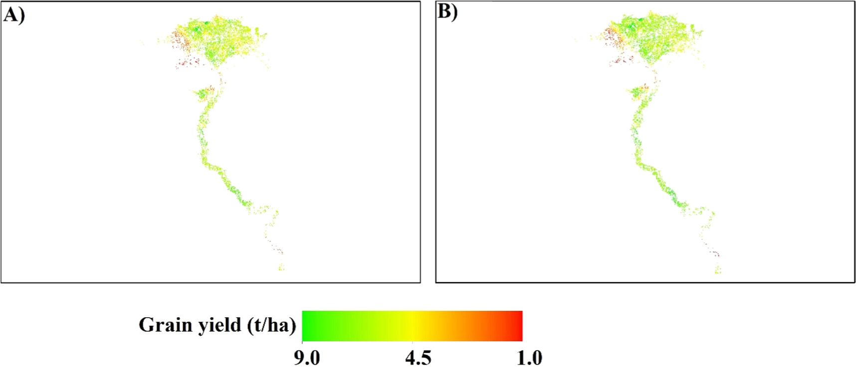
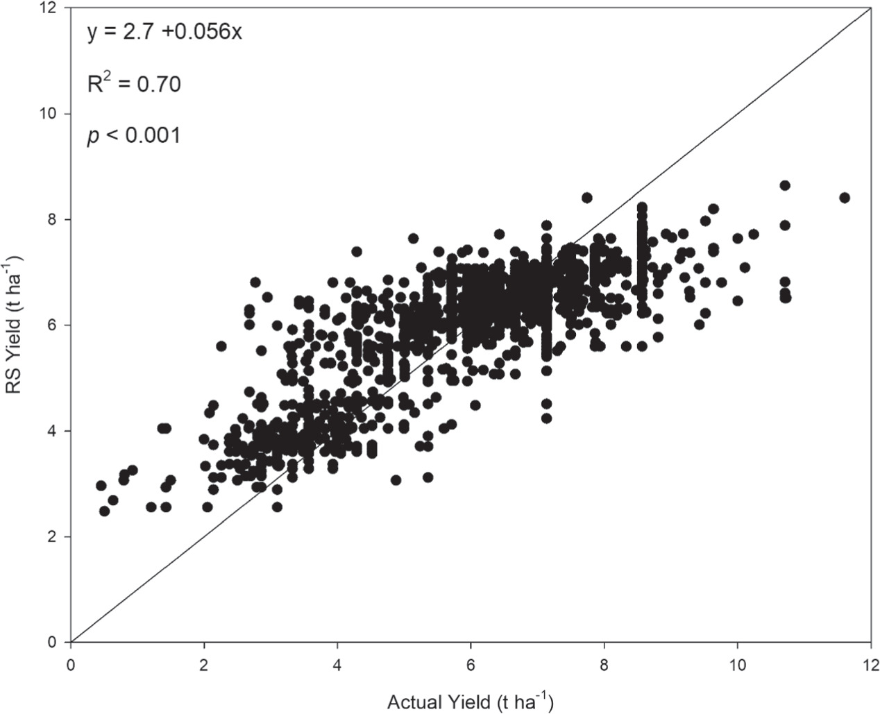
The trained ML models were deployed to predict RS yield using VIs as predictors and actual yield as response. Figures 7 and 8 show that, the AutoML predicted well the spatial wheat yield in Egypt, achieving (R2 = 0.70, P < 0.001) using the stacked ensemble model (figure 5(B)). The ML slightly underestimates the yields relative to the observations, at higher ranges and vice versa in lower ranges. The AutoML approach can be used accordingly to early predict the yield before harvesting, provided that determining the RS indices in the target area. Actual and ML projected yields ranged from 1.0 to 9 t ha−1, with substantial heterogeneity and lower yields in Egypt's northern, western, and southern regions (figure 7).

Figure 7. Spatial distribution of actual wheat yield (A), and remote sensing yield (B) over Egypt during the growing season 2021/2022. Remote sensing yield was predicted using different vegetative indices (figure 4) and the super learner model (stacked ensemble-best of family, figure 5(B)).
Download figure:
Standard image High-resolution image
Figure 8. Actual yield versus remote sensing yield predicted by H2OAutoML approach using different vegetation indices such as NDVI, EVI, GCVI, GNDVI, and WDRVI.
Download figure:
Standard image High-resolution image3.5. Yield change under future climate change
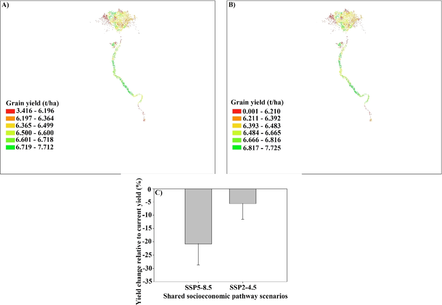
Due to using diverse dataset to train and test the ML, including weather data, the trained models can be deployed for predictions under future climate change scenarios. Exploring the future impacts of climate change on food security may help decision-makers with potential adaptations. Coupled Model Intercomparison Project Phase 6 (CMIP6) scenarios provide valuable information for predicting future climate change. These scenarios are developed by a suite of climate models from research institutions throughout the world, and they predict possible future trajectories of greenhouse gas emissions, land use changes, and other climate-influencing factors. While CMIP6 scenarios offer valuable insights into potential future climate conditions, their coarse resolutions may not be suitable for local or regional impact assessments. Downscaling is a process used to bridge the gap between the coarse resolution of global climate models and the finer scales required for local or regional analysis. Thus, we used here a downscaled GCM under two SSPs in Egypt to explore the climate change impacts using the trained ML model. By replacing maximum and lowest temperatures from the trained weather dataset with those from SSP4.5 and SSP8.5 (Supplementary figure 5), the trained AutoML accurately predicted yield under future climate conditions (figures 9(A) and (B)). The Fossil-Fueled Development scenario (SSP8.5) showed lower spatial yield than the moderate scenario (SSP4.5) over Egypt in the mid century (figures 9(A) and (B)). The results showed that wheat yield is projected to decline by 21% and 5% under SSP8.5 (pessimistic) and SSP4.5 (moderate) respectively during the mid of century, 2050 (figure 9(C)). The uncertainty associated with SSP8.5 was bigger than that in SSP4.5. AutoML is a promising tool for predicting wheat yield using RS signals and under future climate change scenarios, confirming its applicability to update the yield gap mapping platform.
Figure 9. Predicted wheat yield under future climate during the mid century (2020–2050) using two SSPs (SSP2-4.5 (A) and SSP5-8.5 (B) under one GCM (CanESM5) using the super learner model from the developed H2OAutoML approach (stacked ensemble-best of family, figure 5(B)), as well as the change of wheat yield under future climate change scenarios relative to current yield (C). CMIP6 scenarios included one GCM as CanESM5 and two shared socioeconomic pathways (SSPs) as SSP2-4.5 and SSP5-8.5 which downscaled statistically by Kheir et al 2023 for the study area.
Download figure:
Standard image High-resolution image
4. Discussion
The developed approach (AutoML) is very important in yield predictions outperforming the conventional ML, since it is capable of producing a large number of models in a short amount of time [63]. The world population is growing faster, in addition to limited natural resources, a wide disparity between food production and consumption happened, increasing the pressure on food security [71]. Digital agriculture and smart applications such as ML are potential solutions to predict smallholder yields and contribute to enhance their production using site specific recommendations. We therefore developed a novel ML approach (AutoML) to predict yield at scale using diverse dataset. The developed approach was built using multi-sources data (soil, weather, topography, and remote sensing), since heterogeneous data include unique information on crop growth development and yield, improving the crop yield predictions [11, 13, 72]. Although different dataset was considered, AutoML trained rapidly and accurately than conventional ML models, enabling the prediction with large number of models in less time. The important features from AutoML showed that EVI, GNDVI and GCVI outperformed other RS indices (NDVI and WDRVI) in determining wheat yield. There were considerable disparities in VIs selection and yield estimation accuracy due to varied crop growth stages and cultivars [73]. The outperforming of GNDVI and GCVI could be explained by the strong correlation between chlorophyll content and LAI [74, 75]. However, due to land fragmentation in Egypt, and using different cultivars and agronomic practices by smallholder farmers, it is recommended to use all VIs in ML to predict the yield. The lower yield at some Northern, Northern-Western and Southern parts of Egypt (figure 7), is mainly attributed to soil salinity issues at North [34, 76], and higher temperatures in the South [25]. This is another proof supporting our approach which uses heterogeneous data sources include soil and climate in crop yield predictions.
Our research presents an accurate and low-cost framework to predict smallholder production over time way by integrating disparate source data, the GEE platform, and the AutoML technique, which has substantial implications for crop yield forecasting and site-specific management practices. However, like many others, our study has some uncertainties which need to be covered as future directions. Although VIs successfully caught some yield variability, some significant variability remains unaccounted for. Some of these variabilities could be attributed to errors in field survey, cloud cover impacts, aerosol, field size (edge pixel effect), and poor management by smallholders [77, 78]. Statistical measures in Supplementary table 1 revealed that the standard deviation of predicted yield is 1.58, indicating that the data is dispersed around the mean. Furthermore, the mean absolute deviation was 1.07, indicating some fluctuation around the mean. The −0.59 skew indicates a longer left tail. Such heterogeneity can be attributable to field survey data received from farmers using diverse cultivars and management approaches. Moreover, the interacting effects of various uncontrolled environmental and socioeconomic factors might have a significant impact on the results of farm surveys [79]. In addition to survey data variability, there is also variability from other factors such as cloud cover effect on RS signals, as noticed by increasing standard deviation and skews (S. Table 1). All these variabilities contributed to causing the model performance uncertainties. Overall, a novel and robust AutoML approach has been developed achieving satisfactory accuracy and could be applied in other environments to predict smallholder yield using different data sources, rather than using the traditional machine learning approaches [80–82]. The work strengths could be summarized in developing a novel automatic machine learning library for fast, quick, and robust predictions using the maximum number of models include the ensemble model. This is the first paper to develop an automated machine learning approach the agricultural systems worldwide. Furthermore, the trained AutoML was deployed for early yield predictions using RS vegetation indices, achieving robust accuracy. This can help farmers and decision makers for early prediction of yield before harvesting, contributing to preparing economic recommendations for stakeholders. As climate change is a hot spot right now negatively affected global production and food security, the developed approach was deployed for a single GCM and two SSPs in CMIP6 scenarios. Nevertheless, further application of the developed approach with Multiple GCMs in different locations could be a future direction. The application of the trained AutoML models in other geographic conditions with different environments and crop types requires careful consideration of factors such as transfer learning, feature engineering, ensemble learning, adaptive learning, domain adaptation, and collaborative learning. By leveraging these approaches in conjunction with domain knowledge and stakeholder engagement, it is possible to develop more resilient and widely applicable ML solutions for agriculture. Furthermore, integrating this approach with crop models will enhance the yield prediction, taking advantage of process-based models in integrating crop physiological processes and cultivar genetics. Crop models and ML approaches offer distinct methodologies for predicting crop yields, each with its own strengths and limitations. While crop models provide mechanistic insights into crop growth processes and explicit representation of uncertainty, ML models offer flexibility, scalability, and potential for high predictive accuracy. Integrating both approaches can leverage their complementary strengths to enhance yield predictions and better understand the impacts of environmental variability and climate change on agriculture. Crop models and machine learning can be integrated [83] by employing crop model inputs and outputs as predictors in ML, together with other external variables that crop models cannot include, such as salinity, pests, diseases, and terrain, to predict yield at spatial explicit. Therefore, future directions could be done by coupling the developed approach (H2OautoML) with crop models to not only predict the current spatial yield, but also to explore future impacts, adaptation, and mitigation to climate change. This will be taking advantage of each other, and eliminate their limitations, improving the prediction and reducing uncertainty, which is important to policy recommendations for food security and nutrition.
5. Conclusion
Based on multi-source dataset and extensive field surveys over Egypt, we integrated soil, topography, weather, and remote sensing data to build a novel and automatic machine learning approach (AutoML) for estimating smallholder yield. Training and testing were accomplished quickly and accurately using 20 models in the new approach, proving AutoML's outperformance over conventional ML. Considering different VIs as predictors, AutoML predicted yield accurately when compared with actual yield. When compared to traditional correlations, the developed ML approach (AutoML) predicted wheat yield using remote sensing VIs with a high correlation to actual yield. The developed approach also demonstrated the capability of predicting yield under future climate change. This method could be used to forecast yield for stakeholder farms all over the world where ground data is scarce.
Acknowledgments
Authors thank the CGIAR Excellence in Agronomy-Egypt Use Case (https://www.cgiar.org/initiative/11-excellence-in-agronomy-eia-solutions-for-agricultural-transformation/) where this work was conceptualised and is currently being undertaken. We also sincerely acknowledge the CGIAR-INIT-23: Building Systemic Resilience Against Climate Variability and Extreme (Climber project), (Grant Number 200303) for funding. Authors thank the EiA Transform team for fruitful discussions.
Data availability statement
All data that support the findings of this study are included within the article (and any supplementary files).
Conflicts of interest
The authors declare that there is no conflict of interest.
Supplementary data (1.1 MB DOCX)