
Abstract
Efficient and optimal energy transport is one of the present challenges in the physics of many different devices. In this context, the dynamic effective thermal diffusivity of a fluid with a non-Fourier heat conduction law is examined. Considering the simplest description for heat conduction beyond Fourier's law (the Cattaneo-Vernotte equation), an enhancement in the heat transported under oscillating conditions for both Newtonian and Maxwellian fluids may be obtained. The possible impact of such enhancement on the optimization of heat transfer processes and energy efficiency, and hence the importance of searching for fluids obeying the Cattaneo-Vernotte heat transport (specially for use in nanoscales where the effect may have an influential role) are also discussed.
Export citation and abstract BibTeX RIS

Original content from this work may be used under the terms of the Creative Commons Attribution 3.0 licence. Any further distribution of this work must maintain attribution to the author(s) and the title of the work, journal citation and DOI.
1. Introduction
In a world focusing on sustainable development, the search for new strategies to optimize the use of energy is a must. In particular, thermal applications require efficient heat transfer processes. An area in which performance and reliability may depend crucially on temperature conditions is that of telecommunications. In this area, the need for miniaturizing devices and using energy efficient processes has motivated many studies on heat transport at the nanoscale. Recently, one dimensional nanostructured photonic devices involving porous silicon have been used as secondary mirrors for solar concentrators. Although these structures are built considering their high reflectance, they still present dissipation [1] which may lead to very high temperatures when they are functioning. There have also been several studies showing that a diffusion-wave transport appears when heat is transported in small scales [2–5]. Moreover, fluids in narrow containers could have very different behavior in comparison with what they do in the bulk. For instance, at the nanoscale the liquid condensates are layered [6] and their transport properties could present inertia. Particularly for this size scale the heat transport in the regime of second sound [7] could lead to a non-Fourier constitutive equation for the heat flux [8, 9]. Non-Fourier heat transport in the nanoscale has also received a lot of recent attention in connection with the use of many phenomena present in solid systems [10–12].
On the other hand, in the modeling of heat transport for nanosized fluid systems, the inclusion of the elastic properties of the fluid leads to an interesting enhancement in the effective thermal diffusivity not present in the Newtonian case [13]. Thermodynamic analysis is therefore useful in assessing the performance and in guiding research in several applications such as thermoelectric conversion, photovoltaic technology, microelectronics, photonics, heat removal, etc.
One of the different strategies to improve heat transfer in fluid systems is based on the use of an oscillatory flow with no mass transfer, as first proposed by Kurzweg [14]and recently assessed experimentally by Patil and Gawali [15]. In particular, Kurwzeg found that in the oscillatory flow of a Newtonian fluid in a tube the effective thermal diffusivity αe presents a maximum for a given frequency. In the same line of reasoning but with a Maxwellian fluid, AA Lambert et al [13] found that the effective thermal diffusivity can be substantially improved. In this case, several maxima are present at specific resonant frequencies, thus making these fluids excellent candidates to optimize the heat transport. Nevertheless, from the physical point of view, although this work did indeed consider the inertia in the stress tensor, this was not done in the heat transport, where Fourier's heat law was assumed and used in the energy balance equation. This assumption has the nonphysical feature that if a sudden change of temperature is made at some point on the body, it will be felt instantaneously everywhere, though with exponentially small amplitudes at distant points.
It should be noted that fluids tend to behave more like solids on small scales [6] showing inertia and not obeying Fourier's law [16, 17]. Thus, since use of the Maxwell model for viscoelasticity considers thermodynamic inertia for momentum transport but Fourier's law does not consider such thermodynamic inertia, one may take the Cattaneo-Vernotte (CV) equation [7] as an alternative for the simplest model to involve thermodynamic inertia in the heat transport process. Clearly, the relaxation time appearing in the CV equation limits the heat flow velocity to a finite value, which is physically appealing. Nevertheless, we are fully aware that, due to its oversimplification, the CV model may in some instances lead to non-physical results. In any case since, as we will show afterwards, such model will allow us to derive fully analytic results, it is left to experimental confirmation to clarify whether its applicability in this instance is valid. As a matter of fact, very recent papers (a) sample of which may be found in [18–24] deal with many aspects of non-Fourier heat transfer in a variety of transport problems, including some with non-Newtonian Fluids. These studies are very interesting but involve numerical rather than analytic work, as we have done here. We are persuaded that analytic results provide a deeper understanding of the physical phenomena involved. In this sense, we should point out that the resonance frequencies for the Maxwellian case have been reported experimentally in a macroscale, namely a radius tube of 2 cm using cetylpyridinium chloride and sodium salicylate (CPyCl/NaSal) in [25–27]. Of course if we go to small scales water behaves as Maxwellian fluid [6] and we are persuaded that the resonant behavior will appear.
Thus, the main objective of this work is to explore analytically the heat transport modeled by the CV equation in both Newtonian and Maxwellian fluids. This will be done by considering the flow under the action of an oscillatory pressure gradient and also assuming that the fluid is contained in a tube of constant cross section. We will further consider that the fluid at the ends of the tube is at different temperatures and the tube walls are insulated.
The paper is organized as follows. In section 2 we develop the theoretical framework and obtain the velocity and temperature fields using the CV equation to account for heat transport in both a Newtonian and a Maxwellian fluid. Using similar ansatzs to the ones used by Kurzweg [14] and Lambert et al [13], we arrive at analytic expressions for the velocity and temperature fields. In section 3 we compute the effective thermal diffusivity and the dimensionless heat flux. We find that in the Newtonian case multiple maxima appear in the effective thermal diffusivity, for different oscillation frequencies. This is a consequence of using the CV equation for the heat flux in the energy equation. On the other hand, for a Maxwellian fluid we find that the diffusivity may increase in various orders of magnitude with respect to the results derived with Fourier's law and that in this respect the heat flux relaxation time plays an important role. We finish this section by providing useful (approximate) fitting formulas for the maximum frequencies and thermal diffusivities. The paper is closed in the final section with some concluding remarks.
2. Hydrodynamic fields for fluids under oscillatory flow and non-Fourier heat transport
We consider an oscillating incompressible laminar flow of a fluid in a tube of radius a. The oscillatory regime of the fluid is produced by a harmonic pressure gradient applied in the x direction.
The governing equations for this process are [28], the mass conservation equation for an incompressible fluid

the momentum balance equation

and the energy balance equation expressed in general form as

where v, p, τ, T and q are the velocity, the pressure, the viscous stress tensor, the temperature and the heat flux, respectively, while ρ and c are the mass density and the specific heat at constant volume (taken to be a constant), respectively. In equation (3), the viscous dissipation is considered to be negligible because we will restrict ourselves to low Reynolds numbers, where the linear approximation is valid [25]. Also, it is important to stress that we are not considering internal heat production, and as it will be seen below the boundary will produce a heat flow. With these plausible considerations, we may decouple the momentum and energy transport equations.
To solve specific problems we need to consider the corresponding constitutive equations for the viscous stress tensor and the heat flux.
The viscous stress tensor equation depends on the nature of the fluid. For simplicity, we will here consider only the linear Maxwell model, namely,

where η and tm, are the dynamic viscosity of the fluid and the Maxwell relaxation time, respectively, which are also assumed to be constant [29]. The term on the left-hand side of the equation (4) introduces the elastic behavior of the fluid. Note that if tm = 0, the Newtonian fluid limit is recovered. Also note that in equation (4) we only consider the symmetric part of the velocity gradient.
2.1. Velocity field
In order to obtain the velocity field for the oscillatory flow of the linear Maxwell model, the following additional assumptions will be made. The flow is assumed to take place only in the axial direction and the velocity is considered to be independent of the axial coordinate. Further, the flow is far way from the edges, there is no detachment of the boundary layer and cylindrical symmetry holds. This is precisely the system that was examined by Lambert et al [13] but for the sake of completeness we next summarize their derivation.
Given the above assumptions, the velocity field in cylindrical coordinates can be expressed as ![${\bf{v}}=[0,0,v(r,t)]$](https://content.cld.iop.org/journals/2399-6528/2/5/055006/revision2/jpcoaabd9eieqn1.gif) , whereupon the continuity equation for incompressible fluids is satisfied. Further, the nonlinear term
, whereupon the continuity equation for incompressible fluids is satisfied. Further, the nonlinear term  of equation (2) is zero and so the momentum balance equation is transformed into

To obtain an equation for the velocity field we combine equations (5) and (4), namely,

with the following boundary conditions


The first boundary condition establishes that the fluid velocity in the tube center must have a finite value, and the second condition establishes the no slip condition at the tube wall. We now take the pressure gradient leading to the oscillatory flow to be the real part of  , where Px, is the pressure gradient amplitude and ω0, is the constant angular frequency. Next a solution of the form
  is proposed. Thus, from equation (6), V(r) must satisfy

Applying the boundary conditions (7) and (8) in equation (9), one finally arrives at

where J0 is the Bessel function of first kind and zeroth order and we have introduced the auxiliary quantities

and
Note that βv, is a parameter that depends basically on the properties of the fluid. Equation (10) provides the velocity field for a linear Maxwellian fluid inside a tube of constant cross-section undergoing oscillatory motion [30], this expression is in agreement with experiments [25–27]. This velocity field will next be introduced into the energy equation along with the CV equation for the heat flux to obtain the temperature field.
2.2. Temperature field
Our next goal is to determine the heat axial transport across the tube considering the CV equation [7]. In this instance, the heat flux q obeys

where the parameter tq is the relaxation (heat flux) time and κ is the thermal conductivity of the fluid, which are also considered to be constant. It is evident that if tq = 0, Fourier's law of heat conduction is recovered. Clearly, this expression has a similar form to the one for the viscous stress tensor of the linear Maxwell model, equation (4).
Here we can impose the following boundary conditions

where x0 and xf are the initial and final positions and γ is the constant axial temperature gradient averaged in time, according to Kurzweg [31] proposal.
Introducing equations (11) into (3), taking into account that the flow takes place in the axial direction and using the molecular thermal diffusivity α = κ/ρc, one arrives at

This is the temperature equation for the fluid obeying the CV equation under oscillatory conditions. Note that if tq = 0 one recovers the equation for the temperature field considered in [13]. Following Kurzweg [31] and Lambert et al [13] we propose a solution to equation (13) that assumes a constant axial temperature gradient averaged in time γ = ∂ T/∂x, of the form

g(r) being a function that describes the temperature radial dependence [14]. This expression shows a linear behavior on T in the axial direction as well as a time dependent transversal variation as was imposed in equation (12). In this instance, the temperature field satisfies the following boundary conditions in the radial dimension


The first radial boundary condition establishes that the fluid temperature does not diverge at the center of the tube and the second one that the tube wall is thermally insulated. Substituting the temperature field as given in equations (14) into (13) one gets

with

and

Note that βc depends on the fluid parameters. The general solution to the inhomogeneous second order differential equation (17) is of the form

where Y0 is a Bessel function of the second kind and zeroth order, C1 and C2 are constants depending on the boundary conditions. Further gp(r) is the particular solution which is easily derived and turns out to be given by
Therefore, applying the boundary conditions g(0) = finite and  , we finally obtain

where J1 is the Bessel function of first kind and first order. Once equation (18) is substituted into equation (14), the temperature field of the fluid is completely determined. We need to emphasize that this solution is valid for both Newtonian and Maxwellian fluids depending on the form of the parameter βv, and it reduces to the result of [13] if Fourier's heat conduction law is used instead of the CV equation, that is if tq = 0.
We are now ready to analyze the behavior of the effective thermal diffusivity for a linear Maxwellian fluid in which heat transport is governed by the CV equation and under oscillating laminar flow.
3. Effective thermal diffusivity
Once the velocity and temperature fields have been obtained for the fluid under an oscillatory regime, we can now look at the effective thermal diffusivity to calculate the heat transfer from the extreme of the tube at high temperature to its extreme at low temperature.
The effective averaged thermal diffusivity αe may be defined as

where [ ]R denotes the real part. The left-hand side of this expression represents the effective axial thermal flux per unit cross-sectional area and the right-hand side the time-averaged convective thermal flux produced by the interaction of the cross-stream-varying velocity and temperature fields [14]. In agreement with Kurzweg's development, we neglect the small contributions due to the axial thermal conduction. Substituting the real part of the velocity and temperature fields in equation (19) and carrying out the integrals over the angular coordinate and time, we get

where (−) denotes the complex conjugate. By using equations (10) and (18) in (20), we arrive at integrals containing products of Bessel functions which can be performed analytically. In order to compare with previous results, it is convenient to derive the appropriate expression for the tidal displacement Δx that represents the averaged maximum axial displacement that fluid elements travel during half period of oscillation. It is defined by

If the velocity field is introduced into equation (21) with A = πa2, and integration is carried out, we get

As mentioned by Kurzweg [14], in order to avoid the direct convective mass transfer, the value of Δx must be smaller than the distance between the two thermal reservoirs.
The effective thermal diffusivity can be adequately normalized through division by the quantity ω0(Δx)2 yielding
where we have introduced the following dimensionless numbers: the Prandtl number  , the square of the Womersley number
  , the Deborah number
  ,1
and the new Ed number, this latter defined as the quotient between the heat flux relaxation time tq and the viscous diffusion time so that
,1
and the new Ed number, this latter defined as the quotient between the heat flux relaxation time tq and the viscous diffusion time so that  . This number represents the competition between the thermal inertial properties and the diffusive momentum transfer process. Note that in terms of the dimensionless numbers, the arguments of the Bessel functions are given by
and
Equation (23) is the main result of this paper and provides the effective thermal diffusivity in the laminar flow in the axial direction and under an oscillating pressure gradient of a Maxwellian fluid whose transport of heat is governed by the CV equation. It must be emphasized, that from this general result, one can obtain the diffusivity for both a Newtonian (tm = 0) or a Maxwellian fluid (tm > 0) that either obeys Fourier's law (tq = 0) or the CV equation (tq > 0). If tq = 0, this implies that βc reduces to  , which is the corresponding expression for a fluid described by Fourier's law derived in the work by Lambert et al [13].
The information of four different kinds of transport in the system included in equation (23) may be analyzed in terms of the dimensionless numbers as follows. First, (a) when De = Ed = 0 (which means that tq = tm = 0) it reduces to the case analyzed by Kurzweg [14] for a Newtonian fluid obeying Fourier's law. Secondly, (b) if Ed = 0 (which means that tq = 0) but  it reduces to the case of a Maxwellian fluid obeying also Fourier's law [13]. Thirdly, (c) if De = 0 (or equivalently tm = 0) but
  (i.e.
(i.e. ) we have the case of a Newtonian fluid but with a CV equation for the heat flux. Finally, (d) when both De and Ed are not zero (i.e. both
  and
and  ) the complete form provides the thermal diffusivity of a fluid with both thermal and momentum inertia.
In figure 1 we present the normalized effective thermal diffusivity as a function of the Womersley number for a Newtonian fluid (De = 0), with a Prandtl number Pr = 10 and for Ed = 0, 0.5 and 10. In this case it is important to note that a change in qualitative behavior, to our knowledge not reported earlier for Newtonian fluids, appears as Ed increases beyond Ed = 10: there is a huge maximum at a given value of the Womersley number followed by increasingly smaller peaks that die out as Wo increases. This is certainly an effect of the use of the CV equation instead of Fourier's law. A similar qualitative behavior is found for the Maxwellian fluid with Ed = 0 (i.e. if tq = 0) (see figure 2) thus suggesting that such behavior may be present whenever thermodynamic inertia is important, namely when beyond some threshold values either  (
( ) or
) or  (
( ).
).
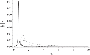
Figure 1. αe/ω0(Δx)2 as a function of the Womersley number Wo with Pr = 10, for different values of Ed: Ed = 0 (dotted line), Ed = 0.5 (dashed line) and Ed = 10 (solid line).
Download figure:
Standard image High-resolution image
Figure 2. αe/ω0(Δx)2 as a function of the Womersley number Wo for a Maxwellian fluid with Pr = 10, De = 0.5, and different values of Ed: Ed = 0 (dotted line), Ed = 0.5 (solid line) and Ed = 1 (dashed line).
Download figure:
Standard image High-resolution imageFigure 2 shows the normalized effective thermal diffusivity for a Maxwellian fluid with Pr = 10, De = 0.5 and for Ed = 0, 0.5 and 1. Here we observe that when Wo < 1.6, the value of the thermal diffusivity is larger in fluids with Ed = 1 (dashed line) and Ed = 0.5 (solid line) than with Ed = 0 (dotted line), but when Wo > 1.6, the value of the diffusivity decreases for these fluids. This behavior is also different to the case in which heat transport of the Maxwellian fluid is governed by Fourier's law: while in both instances one gets several maxima for different values of the Womersley number, when one considers Fourier's law the main peak is the first one and then it is followed by several relative maxima of decreasing height. On the other hand, if the CV equation is used, no clear-cut behavior of the peaks may be ascertained.
This conclusion is reinforced by the results displayed in figure 3 where we show the normalized effective thermal diffusivity for a Maxwellian fluid again with Pr = 10 and De = 0.5 but for Ed = 0, 0.01 and 25. Even for these very different values of Ed no systematic behavior can be inferred.

Figure 3. αe/ω0(Δx)2 as a function of the Womersley number Wo for a Maxwellian fluid with Pr = 10 and De = 0.5, and for three different values of Ed: Ed = 0 (dotted line), Ed = 0.01 (solid line) and Ed = 25 (dashed line).
Download figure:
Standard image High-resolution imageTo better appreciate how the dimensionless effective diffusivity (αe/ω0(Δx)2) changes with varying the Wo and Ed numbers, in figure 4 a three-dimensional graph is shown for the case in which Pr = 10 and De = 0.5. The main conclusion is that as Ed is increased, the effective thermal diffusivity maximum value increases and the frequency at which it appears decreases.

Figure 4. αe/ω0(Δx)2 as a function of the Womersley number Wo and of Ed with Pr = 10 and De = 0.5.
Download figure:
Standard image High-resolution imageFrom the previous discussion it follows that in some cases an improvement in the diffusivity when one uses the CV equation instead of Fourier's law is observed over a certain range of frequencies. But in other ranges they are of equal magnitude. To analyze this behavior more closely, it is convenient to introduce a dimensionless number χ that is the ratio between both diffusivities which we will denote by αCV and αF, respectively (the former being αe as given by equation (23) while latter follows from equation (23) with Ed = 0).
Clearly, χ is a dimensionless number depending on Pr, De, Ed and Wo and may allow us to determine when the dimensionless thermal diffusivity using the CV equation is higher than the one obtained using Fourier's law.
The explicit expression for χ reads
In figure 5, χ is plotted for a fluid obeying the CV equation as a function of Wo, with Ed = 0.16, 0.5 and 0.7 taking Pr = 10 and De = 0.5. Now we observe that when  . This means that at very low frequencies it is difficult to appreciate the effects of thermal inertia included in the CV equation so the resulting diffusivity is very similar to the one obtained with Fourier's law. As Wo is increased, χ also increases to a certain maximum value and then starts to decrease until χ = 1 at a certain value of the Womersley number. Such value of Wo > 0 for which χ = 1, will be hereafter referred to as Wc. Beyond Wc, as Wo is increased, the value of χ becomes smaller (χ < 1), implying that the effective diffusivity obtained with Fourier's law is higher than the one derived with the CV equation.
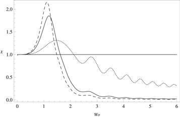
Figure 5. χ as function of the Womersley number Wo for a Maxwellian fluid with Pr = 10 and De = 0.5, and different values of Ed: Ed = 0.16 (dotted line), Ed = 0.5 (solid line) and Ed = 0.7 (dashed line).
Download figure:
Standard image High-resolution imageTo gain further insight into the behavior of χ, we consider now smaller Ed values. In figure 6 χ is plotted as a function of Wo, for Ed = 0.12, 0.06 and 0.01 taking again Pr = 10 and De = 0.5. For Ed = 0.01 and 0.06 (dashed and solid lines, respectively) χ, although with oscillations, is always greater than one for any value of Wo, implying that the effective thermal diffusivity obtained with the CV equation exceeds for these values of Ed the one obtained from the use of Fourier's law. Although not shown in the figure, the same trend is observed for values of Ed ≪ 1, namely for such values χ > 1 across the entire frequency range. On the other hand, when Ed = 0.12 (dotted line) there is a (small) range of frequencies in which χ > 1 but beyond a certain Womersley number χ becomes smaller than one. This trend, in which regions where αCV > αF appear beyond a certain frequency, remains as Ed is further increased (c.f. figure 5).

Figure 6. χ as a function of the Womersley number Wo for a Maxwellian fluid with Pr = 10 and De = 0.5, and different values of Ed: Ed = 0.12 (dotted line), Ed = 0.06 (solid line) and Ed = 0.01 (dashed line).
Download figure:
Standard image High-resolution imageIn order to have a clearer picture of the dependence of χ on both Wo and Ed and its qualitative behavior, in figure 7 a three-dimensional graph is shown for the case of a Maxwellian fluid having Pr = 10 and De = 0.5. In this graph, the plane corresponding to χ = 1 has been explicitly indicated. One finds that, in general, as Ed increases, the value of χ also increases but the range of frequencies where χ > 1 is also reduced.

Figure 7. 3-D plot showing χ as a function of the Womersley number Wo and of Ed for a Maxwellian fluid having Pr = 10 and De = 0.5. The blue plane indicates the region where χ = 1.
Download figure:
Standard image High-resolution imageAs illustrated in figure 5, for Ed ≥ 0.16 one gets a maximum value of χ which increases as Ed is increased. In figures 8, 9 and 10, we display as, functions of Ed, the maximum value χmax, the frequency at which this maximum occurs Wmax and the value of the frequency Wc at which χ becomes 1, respectively. In order to guide the search for systems and frequencies where CV transport could lead to heat transfer advantage, it would be useful to have simple expressions for Wmax, χmax and Wc as functions of Ed. Therefore we have made use of a fitting procedure to obtain, albeit approximately, such expressions for a Maxwellian fluid having Pr = 10 and De = 0.5. They read


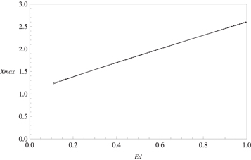
Figure 8. χmax as a function of Ed for a Maxwellian fluid with Pr = 10 and De = 0.5. Values obtained either numerically from equation (24) (solid line) or from curve fitting (dotted line).
Download figure:
Standard image High-resolution image
Figure 9. Wmax as a function of Ed for a Maxwellian fluid with Pr = 10 and De = 0.5. Values obtained either numerically from equation (24) (solid line) or from curve fitting (dotted line).
Download figure:
Standard image High-resolution image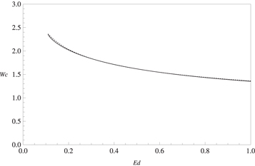
Figure 10. Wc as a function of Ed for a Maxwellian fluid with Pr = 10 and De = 0.5. Values obtained either numerically from equation (24) (solid line) or from curve fitting (dotted line).
Download figure:
Standard image High-resolution image
Clearly, these expressions may prove useful in the search for adequate fluids and scales to observe the enhancement in the thermal diffusivity. The expressions (25), (26) and (27) are valid in the range  . As noted above, below Ed = 0.11, the behavior of χ is not systematic and hence no similar results may be derived.
We can summarize our findings for αCV in the following form:
- For a Newtonian fluid αCV increases as Ed increases; when Ed ≪ 1 a single maximum value is observed and the diffusivity is greater than the one derived from Ed = 0 (heat transport obeying Fourier's law). If Ed ≫ 1 multiple peaks appear, the first one having the greatest height. This behavior is a consequence of considering the CV equation for heat transport, which introduces the relaxation time tq; if tq = 0 (Fourier's law) this feature is not seen.
- For a Maxwellian fluid the presence of the relaxation times tm and tq, significantly modifies the behavior of αCV with respect to that of αF. The ratio of these two quantities, here called χ, provides information about when the diffusivity considering the CV equation is larger, equal or smaller than the one derived from the use of Fourier's law. Such ratio depends on the values of Pr, De, Ed and Wo. As an example, for fixed values of Pr and De, we have illustrated in figure 5, the frequency ranges in which one of the two models of heat transport is superior to the other in terms of leading to a greater effective thermal diffusivity. With information of this kind one may hope to do a proper selection of a fluid if the goal is to optimize a heat transfer process.
To complete the analysis, the next subsection is devoted to a comparison between the heat flow obtained under oscillating conditions and the one obtained from pure molecular diffusion in a stationary regime.
3.1. Quantitative comparison between the oscillatory heat flow and the molecular heat flow
The comparison between oscillatory heat flow and molecular heat flow will be performed by defining Hx as the ratio between the heat flow under oscillatory conditions q0 and the molecular heat flow qm. Here  and
and  . In terms of the dimensionless effective thermal diffusivity
  , Hx is thus given by
Therefore, the heat flow associated to oscillatory motion is  times the molecular heat flow. For values
  , the oscillatory motion leads to an improved heat transfer.
To our knowledge, there have been no reports so far of real fluids obeying the CV equation. Nevertheless, for the sake of illustration, we calculate  for a hypothetical fluid with different values of Ed. In order to introduce real Maxwellian fluids we use an aqueous solution of cetylpyridinium chloride and sodium salicylate (CPyCl/NaSal) [13]. In table 1, the column labeled with ni contains the values of the first maximum of the normalized thermal diffusivity corresponding to each parameter set.
Table 1.
Hypothetical values for  where the fluids properties could give interesting behaviors.
| Ed | Wo | ni |
 (Hz) (Hz) |
Px
|
Δx(m) |

|
|---|---|---|---|---|---|---|
| 0.1 | 0.815 | 8.379 | 5.052 | 10128 | 3.280 × 10⁻³ | 9.568 |
| 1 | 0.815 | 9.271 | 5.053 | 10130 | 3.284 × 10⁻³ | 10.631 |
| 59.7 | 0.814 | 2.625 × 10⁻² | 5.042 | 10085 | 3.238 × 10⁻³ | 3.074 × 10⁻² |
| 174.3 | 0.820 | 4.277 × 10⁻³ | 5.105 | 10341 | 4.916 × 10⁻³ | 7.786 × 10⁻³ |
As we can see with Ed = 0.1 and Ed = 1,  , so that an improvement is obtained in the heat transfer, whereas for Ed = 59.7 and Ed = 174.3,
  , so the opposite happens.
4. Concluding remarks
There is clearly a need to optimize heat transfer processes for a better utilization of energy resources. This naturally leads us to address problems in which clever manipulation may lead to an improvement of the use of these resources. As previous studies have suggested [13, 14], one such possibility is the consideration of oscillating flows instead of stationary ones. These studies have relied on the assumption that heat transport is governed by Fourier's law but, as mentioned above, such an assumption ignores thermal inertia and may lead in some instances to nonphysical behavior.
To explore the consequences of using a heat flux not obeying Fourier's law, we have considered here the Cattaneo-Vernotte equation. This equation involves a relaxation time which limits the speed of propagation of thermal disturbances to have a finite value. The introduction of relaxation times in both the stress tensor and the heat flux may have a great effect on the velocity and temperature fields and thus may also affect the behavior of the effective thermal diffusivity αe. In general, the larger the relaxation times are, the magnitude of the maximum values of the diffusivity also becomes large. This change in the constitutive equations may play an important role specially at the nanoscale level, where non-standard transport may show up [10, 11] .
When employing the CV equation, it can be seen that in a Newtonian fluid the effective thermal diffusivity presents multiple maxima as the relaxation time tq is increased beyond a certain threshold, the first such maximum having the greatest amplitude. This differs from the behavior obtained when the heat flux obeys Fourier's law, in which case only a single maximum is present. In a Maxwellian fluid the effective thermal diffusivity presents various behaviors depending on the magnitude of tq. In this instance it is the magnitude of the quantity χ (given by the ratio of the diffusivity obtained with the CV equation and the one derived from the use of Fourier's law) equation (24), for a determined oscillation frequency, which indicates when the former diffusivity is larger, equal or smaller than the latter. The expressions for χmax, Wmax and Wc, corresponding to the maximum value of χ for Pr = 10 and De = 0.5 as a function of frequency, the frequency at which this maximum occurs and the frequency at which χ = 1 (c.f. equations (25), (26) and (27)), respectively, are of great simplicity and these and similar expressions (derived for other combinations of (fixed) Pr and De), may prove useful to assess the expected behavior of a given fluid, thus enabling one to make an appropriate selection to increase the heat transfer in a particular process.
Given the recent interest in high frequency oscillatory flows for micro or nanoscale applications in which rheological behavior is manifested, we hope that the consequences of considering a non-Fourier heat transfer as derived in this paper may provide new insights into the use of oscillatory flows at small scales. We also hope that our results may encourage further experimental work and identification of fluids obeying the Cattaneo-Vernotte equation in which our predictions might be tested and applied.
Acknowledgments
This work was supported by CONACyT under 'Fronteras 367' project.
Footnotes
- 1
The Prandtl number is the ratio between the momentum diffusivity and the thermal diffusivity, the Womersly number represents the relationship between the frequency of the oscillating flow and the viscous effects, and the Deborah number is the ratio between the Maxwell relaxation time and the characteristic viscous diffusion time.