

Abstract
We review some of the recent efforts in devising and engineering bosonic qubits for superconducting devices, with emphasis on the Gottesman–Kitaev–Preskill (GKP) qubit. We present some new results on decoding repeated GKP error correction using finitely-squeezed GKP ancilla qubits, exhibiting differences with previously studied stochastic error models. We discuss circuit-QED ways to realize CZ gates between GKP qubits and we discuss different scenarios for using GKP and regular qubits as building blocks in a scalable superconducting surface code architecture.
Export citation and abstract BibTeX RIS

Original content from this work may be used under the terms of the Creative Commons Attribution 4.0 licence. Any further distribution of this work must maintain attribution to the author(s) and the title of the work, journal citation and DOI.
1. Introduction
There has been a recent surge in interest in bosonic error correction, both from the experimental as well as from the theoretical side. By bosonic quantum error correction we mean the representation of a qubit as a two-dimensional subspace of an oscillator, a means of performing some error correction on this qubit, as well as a suite of techniques to perform universal computation on the qubit.
We review some of these recent developments and older proposals, with an eye towards integration of the ideas into a scalable (code) architecture. To be concrete, we concentrate on superconducting devices as physical realizations, due to the excellent control and engineerability of strong non-linearities, as described by the formalism of circuit quantum electrodynamics (circuit-QED). For more background, we refer the reader to a recent review of circuit-QED [1] and also the realization of quantum error correction in circuit-QED [2].
Due to the commonality of the quantum optics language, some of our discussion applies more generally to other physical systems realizing oscillators, such as optical modes or mechanical oscillators. Our paper does not aim to be comprehensive in reviewing all possible bosonic codes, but rather seeks to identify some promising approaches and future work to be undertaken, in particular emphasizing scalable bosonic GKP error correction.
A first condition to even consider encoding a qubit into an oscillator is that a high-Q oscillator is available 6 . Examples of such high-Q oscillators are microwave cavity modes, of 3D or co-planar resonators in a frequency range f = 3–10 GHz where single-photon life-times can be up to τ = 1/κ = 1–10 ms [3, 4]. Thus, without additional couplings and drives, the native noise model of such microwave cavities is simply photon loss, governed by the cavity decay rate κ.
In order to prepare and manipulate an encoded qubit as prescribed by some code, one induces additional errors which the chosen code should, ideally, also be able to correct. It is thus important to pick a code in which computational manipulations and error corrections are relatively simple and the chosen code can also handle the errors which occur in these processes. As is well known, no finite code can correct all errors, and hence the goal of bosonic quantum error correction is simply to provide a logical qubit which can be used as a building block in a further coding scheme. The repetition or surface codes are the simplest examples of such further encoding steps, using then multiple oscillators.
Even though we can embrace the surface code as the simplest scalable 2D coding scheme [5], variants on who is playing the role of data and ancilla qubit and what additional error correction on these qubits takes place, are important in actually getting the very demanding engineering it, to pan out. If we have learned anything over the past 20 years of Hamiltonian engineering it is that partially-coherent dynamics can be implemented in many quantum systems, while very few to none may allow for the high-precision control and scalability needed for quantum error correction.
Overall, the challenges of efficiently using a bosonic qubit encoding are in (1) keeping the harmonicity of the oscillators as high as possible while temporally coupling to this mode, with high on/off ratio, to create and manipulate non-classical code states, (2) finding a photon number regime in which approximations of engineered Hamiltonians are accurate while the error correcting properties and benefits of the encoding are valid. When using bosonic qubits as basic qubits in a code architecture, it may be advantageous to choose data qubits differently than ancilla qubits and we will give some examples of such choices. The simplest encoding of a single qubit into a bosonic mode can be done using Fock states: the vacuum state represents the logical |0⟩, denoted as  , and a single-photon state represents the logical |1⟩, denoted as
  .
.
For superconducting devices one can view the difference between bosonic encoding versus the regular transmon qubit encoding [6] as an interchange between the roles played by the anharmonic and the harmonic oscillator. Using transmon qubits to store information, resonators are used as couplers and for read-out. Using bosonic qubits to store information, anharmonic oscillators can be used for state preparation and couplers generating effective nonlinearities to realize gates. In this review we will refer to systems in which the lowest two energy eigenstates (in the absence of couplers) are used as regular qubits: this definition covers a Fock encoding as well as a transmon or a fluxonium qubit.
1.1. Preliminaries & notation
Here we collect a few definitions and mathematical identities that are used throughout the paper. Additionally, useful textbooks for quantum optics and its mathematical description are [7–9]. We use  and
and  , where a (a†) are annihilation (creation) operators, so that
 ![$\left[\hat{q},\hat{p}\right]=\mathrm{i}I$](https://content.cld.iop.org/journals/2058-9565/5/4/043001/revision4/qstab98a5ieqn6.gif) and we sometimes refer to
and we sometimes refer to  and
and  as quadratures. A displacement in phase space is denoted as D(α) = exp(αa† − α*a) and acts as D†(α)aD(α) = a + α, while a coherent state is defined as
  . We have
  so that
  . The following identities hold

so that

A single-mode squeezing transformation is given by  with Hamiltonian
  with
with  . The squeezer enacts the mode transformation aout = Sq†(ξ)aSq(ξ) = a cosh(r) − a† eiθ
sinh(r) with r = |ξ| and θ = arg(ξ).
. The squeezer enacts the mode transformation aout = Sq†(ξ)aSq(ξ) = a cosh(r) − a† eiθ
sinh(r) with r = |ξ| and θ = arg(ξ).
In Lindblad equations we use the notation  for some operator A.
It is standard to denote gates acting on a logical qubit subspace with overlines, i.e.  etc. In order to avoid notation clutter, only in section 2.3.2 we denote logical gates on the GKP codewords without it, i.e. CNOT and Z instead of
  and
and  .
.
2. Bosonic qubits and their components
2.1. Early birds & cats and their generalizations
The first bosonic codes were formulated in [10] and designed to protect against photon loss. Of particular interest is a two-mode code with codewords

with |k⟩ denoting a Fock state with k photons. If either  or
or  (or both) were hit by the loss of a single photon on any one of the two modes, we can readily see that the resulting states would still be orthogonal. This orthogonality is a prerequisite for being able to correct the photon loss error, but it is not a sufficient condition. To examine the error correction capability of a (bosonic) code, one asks whether a set of dominant errors satisfies the quantum error correction (QEC) conditions [11] of the code: if this holds (approximately) then there is an (approximate) recovery operation undoing these dominant errors. For a set of errors E = {E1, ..., Ek
} acting on the encoding of a single qubit, the quantum error conditions are as follows. ∀i, j, we require
(or both) were hit by the loss of a single photon on any one of the two modes, we can readily see that the resulting states would still be orthogonal. This orthogonality is a prerequisite for being able to correct the photon loss error, but it is not a sufficient condition. To examine the error correction capability of a (bosonic) code, one asks whether a set of dominant errors satisfies the quantum error correction (QEC) conditions [11] of the code: if this holds (approximately) then there is an (approximate) recovery operation undoing these dominant errors. For a set of errors E = {E1, ..., Ek
} acting on the encoding of a single qubit, the quantum error conditions are as follows. ∀i, j, we require


To examplify the use of these conditions, let us first look at the single-mode version of the code in equation (3):

This code was introduced in [12] as the smallest member of a family of so-called binomial codes, hence its name kitten or 'baby-binomial' code. This code and its logical gates has been implemented using a superconducting microwave cavity mode as an oscillator in reference [13], but the life-time of the encoded qubit was comparable to that of a Fock state encoding. One can easily check that for the error set  , the QEC conditions in equations (4) and (5) for this code are met. However, these errors are only an approximation of the real noise. A photon loss channel with photon decay rate κ lasting for time t with γ ≡ κt ≪ 1, can be modeled by a superoperator
  with Kraus operators
  and
and  , or
, or

For the Kraus operators E0 and E1 the QEC conditions in equations (4) and (5) are not quite met. In particular, we have

as  is an eigenstate of a†
a, while
is an eigenstate of a†
a, while  is not. This means that upon the detection of no photon loss (corresponding to E0) the code states undergo an irreversible distortion. The two-mode version of this code, equation (3), improves on this distortion issue as the quantum error correction conditions for the two mode code are met for the error set
  . These error operators can be viewed as the three Kraus operators of a process in which there is either photon loss on mode a, photon loss on mode b, or no photon loss on either modes. For the states in equation (3) we have no distortion upon not detecting a photon from either modes as
  and
and  are both eigenstates of
  with eigenvalue exp(−2γ). As far as we know, this two-mode code is still awaiting experimental realization.
By allowing ourselves code states with higher average photon number, we can correct for more loss errors, as well as gain and dephasing errors. More precisely, reference [12] has introduced families of binomial and so-called cat codes which correct against the set of errors  for arbitrary L, G and D. For example, the idea behind the binomial codes can be understood as follows. Using the Holstein–Primakoff transformation a†
a → Jz
+ J, the binomial code words
for arbitrary L, G and D. For example, the idea behind the binomial codes can be understood as follows. Using the Holstein–Primakoff transformation a†
a → Jz
+ J, the binomial code words  and
and  can be seen as spin-eigenstates of Jx
= ±J with 2J = N + 1, where one defines N = max(L, G, 2D). Dephasing errors
can be seen as spin-eigenstates of Jx
= ±J with 2J = N + 1, where one defines N = max(L, G, 2D). Dephasing errors  , m = 1, ..., D thus lead to a change in Jx
by at most D ⩽ ⌊J⌋, hence keeping codewords orthogonal. At the same time, protection against photon loss and gain is achieved by using a subspace of sufficiently separated Fock states stabilized by the operator ΠS = ei 2 π a† a/ (S+1) with S = L + G. For S = 1 this gives the photon parity operator
, m = 1, ..., D thus lead to a change in Jx
by at most D ⩽ ⌊J⌋, hence keeping codewords orthogonal. At the same time, protection against photon loss and gain is achieved by using a subspace of sufficiently separated Fock states stabilized by the operator ΠS = ei 2 π a† a/ (S+1) with S = L + G. For S = 1 this gives the photon parity operator  : the even-photon codewords in equation (6) are clearly +1 eigenstates of this photon parity operator.
Another family of single-mode codes are the cat codes. A very simple encoding is  and
and  with coherent state |α⟩, first proposed in [14, 15]. Since |α⟩ and |−α⟩ are not orthogonal, it is more appropriate to define the code states as
  with N± = 2(1 ± exp(−2|α|2)). These states are orthogonal for all α and we can define
  . On this encoding, photon loss induces immediate phase-flip errors since
  . Thus the phase-flip error rate (probability per unit time) is proportional to κ|α|2 with κ the photon loss rate of the encoding mode.
On the other hand, for large enough α, bit-flips, α ↔ −α, can be expected to occur at a much lower error rate as they correspond to a large change of the state in phase space. Particularly interesting is the engineering of Hamiltonians or dissipative processes which have these code states |±α⟩ as degenerate fixed-points, so that there is a 'macrosopic' energy barrier to transition between them, leading to a bit flip rate exponentially small in |α|2. This design can lead to a qubit for which the noise is biased as phase-flip errors are more prominent than bit-flip errors. We will discuss this noise-biased qubit in more detail in section 2.2.
The next-level cat encoding was introduced in [15, 16], and is sometimes referred to as the four-legged cat code since its codewords have four blobs in phase space:

Using the standard identity  one can verify the orthogonality of these two states. As for the kitten code, we can verify that both states are +1 eigenstates of the photon parity operator
  using that Πphoton|α⟩ = |−α⟩. The photon parity thus functions as a check operator, taking eigenvalue +1 on the code space and measuring it is a natural way to detect photon loss and perform error correction.
The states  and
and  , both having even photon parity, are however distinguished by their photon parity modulo 4, expressed as the ±1 eigenvalues of the operator
  . To measure the photon parity operator via an ancilla qubit, a cavity mode-qubit dispersive interaction −χZa†
a/2 can be used [7]. In circuit-QED the interaction Za†
a comes about naturally as the effective interaction between, say, a cavity mode and a linearly-coupled, off-resonant, transmon qubit mode [6]. The measurement of Πphoton then proceeds by preparing the ancilla qubit in |+⟩, letting the interaction take place for time t = π/χ and subsequently measuring the qubit in the |±⟩ basis. Using a transmon qubit and cavity mode, reference [17] has shown that tracking the photon parity by repeated measurements of Πphoton makes for a logical qubit which has a longer life-time than a Fock qubit without error correction in the same cavity mode. This result has essentially been the first demonstration of quantum error correction lengthening the life-time as compared to that of native qubits (transmon and/or Fock encoding) in the hardware.
. To measure the photon parity operator via an ancilla qubit, a cavity mode-qubit dispersive interaction −χZa†
a/2 can be used [7]. In circuit-QED the interaction Za†
a comes about naturally as the effective interaction between, say, a cavity mode and a linearly-coupled, off-resonant, transmon qubit mode [6]. The measurement of Πphoton then proceeds by preparing the ancilla qubit in |+⟩, letting the interaction take place for time t = π/χ and subsequently measuring the qubit in the |±⟩ basis. Using a transmon qubit and cavity mode, reference [17] has shown that tracking the photon parity by repeated measurements of Πphoton makes for a logical qubit which has a longer life-time than a Fock qubit without error correction in the same cavity mode. This result has essentially been the first demonstration of quantum error correction lengthening the life-time as compared to that of native qubits (transmon and/or Fock encoding) in the hardware.
Before we discuss further generalizations, let us examine the quantum error correction conditions, equations (4) and (5) for this cat code with respect to the set of errors  . One can quickly observe that all conditions are obeyed except
  . Besides the uninteresting case of taking α very large (so that all |±α⟩, |±iα⟩ are orthogonal), this last condition is exactly met at sweet spots given by the equation tan α2 = −tanh α2. The smallest sweet-spot at |α|2 = 2.34 lies close to the number of photons
  of the cat code used in the experiment [17].
There are several error channels which impact the performance of the cat code using repeated photon parity measurements. First of all, the code cannot fully correct against the photon loss channel as it cannot correct the distortion Kraus operator E0 = I − γa†
a/2. Secondly, two photon-loss events ∝ a2 implement a logical bit-flip  . Thirdly, photon loss in combination with the inevitable Kerr nonlinearity
  on the cavity mode causes incorrectable dephasing: the Kerr interaction makes the cavity rotation speed depend on the number of photons in the cavity, but this number becomes indeterminate in the presence of photon loss. Last but not least, transmon qubit decay during the qubit controlled-a†
a interaction, is a serious source of feedback error. For example, when the qubit decays half-way through the interaction, |1⟩ → |0⟩, it applies only half the rotation on the cavity mode. The result is that the eigenvalues of
on the cavity mode causes incorrectable dephasing: the Kerr interaction makes the cavity rotation speed depend on the number of photons in the cavity, but this number becomes indeterminate in the presence of photon loss. Last but not least, transmon qubit decay during the qubit controlled-a†
a interaction, is a serious source of feedback error. For example, when the qubit decays half-way through the interaction, |1⟩ → |0⟩, it applies only half the rotation on the cavity mode. The result is that the eigenvalues of  are measured via the qubit measurement, collapsing the logical state.
This last feedback error problem is an important issue for any bosonic qubit, and it has been a central theme in the theory of fault-tolerant computing in general [18]. A disadvantage of the theoretical schemes for fault-tolerant quantum error correction is that they typically require additional hardware resources, such as logical ancilla qubits or (verified) multi-qubit GHZ states. Instead, we may seek hardware-efficient mitigation of the feedback error problem. As an example, reference [19] has addressed the feedback error due to transmon relaxation by drive-engineering the dispersive coupling Hamiltonian to equal −χ(|2⟩⟨2| + |1⟩⟨1|)a†
a and starting the ancilla transmon qubit in the state  . Transmon qubit decay from 2 → 1 then commutes with the transmon–cavity interaction and does not cause errors on the cavity mode. The decay does—as in the normal case—affect the reliability of the transmon qubit measurement outcome. All-in all, this has led to an overall factor 5 in improvement of the life-time of the encoded cat qubit [19].
Another way of minimizing feedback errors on a bosonic code is to use a biased-noise ancilla qubit (section 2.2) as an ancilla qubit. As proposed in reference [20], the goal is then to let the strong-noise error channel affect the ancilla qubit measurement, while the low-noise (bit-flip) channel on the ancilla feeds back low-noise to the bosonic code.
Single-mode cat codes with higher-photon numbers can be formulated and form a class of codes [12, 21]. Reference [22] studied the performance of binomial, cat and GKP codes (see section 2.3), against photon loss, assuming optimal noisefree recovery as permitted by the quantum error correcting conditions. Reference [23] has formulated a general framework of rotation-symmetric codes of which the binomial and cat codes are subclasses: the unifying theme is rotation symmetry of the code states in phase space captured by invariance under the operator ΠS . Another interesting class of bosonic codes uses a three-wave mixing χ(2)-interaction, equation (32), as the central element for defining the code and correcting photon loss [24]. Various classes of multi-mode codes against photon loss exist, see for example [22, 25, 26] and references therein.
A challenge in using a bosonic qubit is that some computational manipulations can be more involved than for a regular qubit. For example, on a regular qubit such as a transmon qubit, rotations by an angle θ around axes X or Y are easily accomplished by temporarily supplying microwave radiation. On a bosonic qubit, these simple single-qubit gates can be non-trivial. An advocated solution in reference [27] is to always use a dual-rail (dr) encoding of a bosonic qubit with  and
and  , where
  and
and  are the states of (an arbitrary) bosonic qubit itself. Having mapped the Bloch-sphere of a qubit onto a two-mode state space, the exponential mode-SWAP operator exp(iθSWAPa,b
) becomes a universal gate to do single-qubit and two-qubit gates, and has been realized in [28]. Here the linear SWAPa,b
transformation interchanges two modes a and b, i.e. its action on quadrature operators for the modes is given by qa
↔ qb
and pa
↔ pb
. If we envision using a bosonic qubit as a building block qubit in a stabilizer code, it is however not necessary to perform any gate, but rather we can focus on performing CNOT or CZ, Hadamard (H) and T gates possibly using ancilla qubits, see e.g. reference [5].
are the states of (an arbitrary) bosonic qubit itself. Having mapped the Bloch-sphere of a qubit onto a two-mode state space, the exponential mode-SWAP operator exp(iθSWAPa,b
) becomes a universal gate to do single-qubit and two-qubit gates, and has been realized in [28]. Here the linear SWAPa,b
transformation interchanges two modes a and b, i.e. its action on quadrature operators for the modes is given by qa
↔ qb
and pa
↔ pb
. If we envision using a bosonic qubit as a building block qubit in a stabilizer code, it is however not necessary to perform any gate, but rather we can focus on performing CNOT or CZ, Hadamard (H) and T gates possibly using ancilla qubits, see e.g. reference [5].
2.2. Noise-biased cat qubit
A method to set up a dissipative process which stabilizes the coherent states |±α⟩ was devised in [15]. The idea is to engineer the Lindblad equation (in a frame rotating at the mode frequency):

with  where
where  with
with  proportional to the strength of a pumped microwave mode acting as a classical field. To understand the fixed points of this evolution—ρ for which
  —we can write the Lindblad equation as

with  . We can then use, with
  :
:

This immediately implies that the states  are fixed points of the Lindblad evolution, as Mα
|±α⟩ = 0, and the last term in equation (11) is canceled by the constant
are fixed points of the Lindblad evolution, as Mα
|±α⟩ = 0, and the last term in equation (11) is canceled by the constant  which remains from the first term. Hence, any linear combination of the states
  is a fixed point of the dynamics.
When the pump inducing the squeezing Hamiltonian Hsq is off,  , we can observe that the Fock states
  and
and  are fixed points, distinguished by their photon parity. Thus when
  is gradually increased, we can smoothly change from a Fock encoding into the cat
  encoding. Photon loss at rate κ, which can be modeled by introducing an additional term
  in equation (10), causes phase-flip errors, i.e. flipping between the states
  , but does not interfere with the stabilization itself as |±α⟩ are eigenstates of a so that
  . One can add a drive term Hdrive =
  (t)a† + *(t)a to the Lindblad equation and observe that the annihilation operator a will generate rotations around the Z-axis (periodically interchanging
  ). At the same time, a† in principle leads to a departure from the qubit subspace spanned by |±α⟩ corresponding to leakage. However, due the ∼|α|2 gap of the Lindbladian, such departure from the eigenvalue-0 manifold is exponentially suppressed and the effect of the driving term can be analyzed by projecting it onto the stabilized subspace. In this subspace it then induces Rabi oscillations around an axis which is exponentially-closely aligned with the Z-axis, with Rabi frequency Ω ∝ |||α|, experimentally demonstrated in [29].
7
A measurement in the X-basis can be accomplished by measuring the photon parity through a coupled transmon qubit. The (pumped) squeezing interaction and the required two-photon dissipative process have first been experimentally realized in [31]. This was achieved by coupling a 3D storage cavity (at frequency ωa
) via a bridging transmon to a lossy cavity (at different frequency ωb
) and applying a two-tone drive on the lossy cavity so as to set up a process to convert two storage photons to one lossy cavity photon which is subsequently lost (the
). At the same time, a† in principle leads to a departure from the qubit subspace spanned by |±α⟩ corresponding to leakage. However, due the ∼|α|2 gap of the Lindbladian, such departure from the eigenvalue-0 manifold is exponentially suppressed and the effect of the driving term can be analyzed by projecting it onto the stabilized subspace. In this subspace it then induces Rabi oscillations around an axis which is exponentially-closely aligned with the Z-axis, with Rabi frequency Ω ∝ |||α|, experimentally demonstrated in [29].
7
A measurement in the X-basis can be accomplished by measuring the photon parity through a coupled transmon qubit. The (pumped) squeezing interaction and the required two-photon dissipative process have first been experimentally realized in [31]. This was achieved by coupling a 3D storage cavity (at frequency ωa
) via a bridging transmon to a lossy cavity (at different frequency ωb
) and applying a two-tone drive on the lossy cavity so as to set up a process to convert two storage photons to one lossy cavity photon which is subsequently lost (the  process). The lossy cavity is driven at pump frequency ωp
= 2ωa
− ωb
as well as close to its own frequency ωb
, generating, through the transmon nonlinearity, an effective degenerate parametric oscillator with resonant terms of the form
process). The lossy cavity is driven at pump frequency ωp
= 2ωa
− ωb
as well as close to its own frequency ωb
, generating, through the transmon nonlinearity, an effective degenerate parametric oscillator with resonant terms of the form  .
.
A more recent experimental realization in reference [32] has been able to cleanly generate the desired interactions (via an effective three-wave mixing, see also section 3.3) and observe the exponential decrease of the bit-flip error rate in |α|2 as well as the linear increase of the phase-flip error rate with |α|2.
An alternative, non-dissipative, route towards a noise-biased qubit was first proposed in [33]. Instead of invoking dissipation, the idea is to engineer a Hamiltonian which has |±α⟩ as degenerate eigenstates, using a Kerr nonlinearity and squeezing. The two-photon dissipation is then considered an optional add-on which helps in mitigating leakage, i.e. a departure from the subspace spanned by |±α⟩. The target Hamiltonian (in the rotating frame of the cavity mode) is

The spectrum of H has eigenvalues running from  downwards as the first term in H is negative-semi-definite. Omitting the factor
  , the highest eigenstates are the states |±α⟩ with degenerate zero eigenvalues. We can observe the similarity and difference with equation (12): here we consider a Hermitian matrix and the phase of the pump amplitude
  is variable and determines the phase of the coherent states which are the zero energy eigenstates. Thus, by adiabatically changing the phase of
  we move to different zero energy eigenstates, allowing us to transform α → −α and hence realize a X gate on
  . For the stability of the encoded space it is important to understand the spectrum of H and the gap below these degenerate zero eigenstates, see the analysis in [20, 33]. To understand this, assume that the phase φ = 0 for simplicity. We can displace the Hamiltonian by D(±α) with
  . For large
  , one can approximate D†(±α)HD(±α) ≈ −4K|α|2
a†
a, a harmonic oscillator Hamiltonian. This shows that for large α, the spectrum approximately has the gap 4K|α|2 and the first excited states below |±α⟩ are roughly equal to D(±α)|1⟩. The so-called 'Cassinian' Hamiltonian in equation (13) was first studied in [34]: the surfaces of constant classical energy are described by Cassinian ovals in ⟨p⟩ and ⟨q⟩ with the focii of the ovals at
, one can approximate D†(±α)HD(±α) ≈ −4K|α|2
a†
a, a harmonic oscillator Hamiltonian. This shows that for large α, the spectrum approximately has the gap 4K|α|2 and the first excited states below |±α⟩ are roughly equal to D(±α)|1⟩. The so-called 'Cassinian' Hamiltonian in equation (13) was first studied in [34]: the surfaces of constant classical energy are described by Cassinian ovals in ⟨p⟩ and ⟨q⟩ with the focii of the ovals at  . As a quantum system the spectrum is that of an inverted double-well ('double-oscillator') with the well maxima at zero energy for the states |±α⟩. We can consider the effect of driving and several dissipative processes for the Hamiltonian in equation (13). For example, when one includes photon loss
  in the Lindblad equation and the pump amplitude is sufficiently large, i.e.
  [33, 35, 36], the fixed point of the Lindblad equation is the state
  with modified
  ,
,  . In this regime the system neatly represent the dissipative storage of a classical bit.
The effect of other sources of noise such as dephasing ( , see also equation (29)), photon gain (
 ) due to the coupling with a finite temperature heat bath, as well coupling with baths with other spectral densities are discussed in detail in [15, 20, 33, 37].
Reference [30] has implemented the Kerr-cat Hamiltonian in equation (13) and the corresponding qubit in the resonant mode of a so-called SNAIL element (see section 3.3), coupled to a read-out cavity mode. The fourth-order nonlinearity of the SNAIL element gives the wanted −Ka†2
a2 term, while one can drive the mode at twice its frequency so as to use the third-order SNAIL term  to turn on squeezing. The experiment generated cat states with |α|2 ≈ 2.5 with a dephasing life-time of 3 μs, and an enhanced decay life-time of 105 μs, and a π/2 rotation around the Z-axis obtained by driving took 24 ns. The ability to convert the noise-biased qubit to a Fock encoding by turning off the squeezing drive allows to measure Pauli X via a standard dispersive measurement [30]. One can also measure a noise-biased qubit in the X-basis by dispersively coupling (−χa†
aZ/2) it to an ancilla qubit to map the photon parity onto the state of the ancilla qubit which is subsequently measured. To realize a (nondestructive) Pauli Z measurement, distinguishing ±α, reference [30] had applied, besides the squeezing drive, a drive at the difference frequency of the SNAIL mode and the read-out cavity mode (b) to get a resonant beam-splitting interaction ∝ a†
b + ab†. The upshot is that the coherent states |±α⟩ are mapped to corresponding coherent states in the cavity mode which are heterodyne-measured when leaking out of the cavity.
to turn on squeezing. The experiment generated cat states with |α|2 ≈ 2.5 with a dephasing life-time of 3 μs, and an enhanced decay life-time of 105 μs, and a π/2 rotation around the Z-axis obtained by driving took 24 ns. The ability to convert the noise-biased qubit to a Fock encoding by turning off the squeezing drive allows to measure Pauli X via a standard dispersive measurement [30]. One can also measure a noise-biased qubit in the X-basis by dispersively coupling (−χa†
aZ/2) it to an ancilla qubit to map the photon parity onto the state of the ancilla qubit which is subsequently measured. To realize a (nondestructive) Pauli Z measurement, distinguishing ±α, reference [30] had applied, besides the squeezing drive, a drive at the difference frequency of the SNAIL mode and the read-out cavity mode (b) to get a resonant beam-splitting interaction ∝ a†
b + ab†. The upshot is that the coherent states |±α⟩ are mapped to corresponding coherent states in the cavity mode which are heterodyne-measured when leaking out of the cavity.
Given that the noise-biased cat qubit is designed to have a low bit-flip error rate, it can function as an ancilla control qubit in the error correction circuit for another code [20] inducing low feedback noise. Assume we have a code which is an eigenspace of a stabilizer S = eiA
and S is to be measured using the noise-biased cat qubit to detect or correct errors. This requires an interaction of the noise-biased cat qubit and the code of the form Hint ∝ (a + a†) ⊗ A since a + a† ≈ Z on the noise-biased cat code space (besides some leakage), allowing for a qubit controlled-S operation. For example, for the cat code,  , requiring a tunable photon–pressure coupling between the two modes of the form Hint ∝ (a + a†)b†
b. For the GKP code, see section 2.3, S is a displacement so that Hint can be chosen to be a tunable beam-splitting interaction of the form a†
b + ab†.
, requiring a tunable photon–pressure coupling between the two modes of the form Hint ∝ (a + a†)b†
b. For the GKP code, see section 2.3, S is a displacement so that Hint can be chosen to be a tunable beam-splitting interaction of the form a†
b + ab†.
It has been argued that, if the noise-bias of this qubit is sufficiently strong, only a classical repetition code [38] might suffice to correct for the dominant phase-flip (Z) errors due to photon loss. Crucial in this idea is that the CNOT gate which is needed to measure the XX checks of this code preserves the noise-bias, that is, Z errors during the gate do not propagate to become X errors after the gate. For the Kerr-cat qubit a noise-bias preserving CNOT gate has been proposed in [37]. A similar idea is to use this Kerr-cat qubit as a basic qubit in a surface code architecture in which the XXXX and YYYY checks are measured [37, 39]. In this modified form of surface code one gains much more information about Z errors. It has been shown that when the probability for phase-flip errors and measurement errors is a factor 100 more than that of bit-flip errors within a phenomenological error model, the threshold against Z errors can be as high as 5% [39]. It is an open question whether such high bias will be feasible in practice as experiments for doing the CZ gate and the noise-bias preserving CNOT gate on these noise-biased qubits are still to come.
2.3. The GKP qubit
The (square) Gottesman–Kitaev–Preskill (GKP) qubit introduced in reference [40] is defined through two commuting displacement operators, acting as translations in phase space, i.e.  and
and  .
8
The ideal GKP code is the space invariant under these two phase-space translations. As a result, any wave function in q (resp. p) in this space has support on
.
8
The ideal GKP code is the space invariant under these two phase-space translations. As a result, any wave function in q (resp. p) in this space has support on  (resp.
  ) for integers
  . The logical operators of the qubit are
  and
and  with
with  . In addition,
  . This choice makes the wave function in q of
  a sum of delta functions at values of q which are even multiples of
  , while
  has uniform support on values of q which are odd multiples of
  . The ideal code meets the quantum error correction conditions for a continuous set of 'at most half-logical' displacements
  , since any products of these shifts maps a
  onto a state orthogonal to both
  and
and  (and vice-versa). The set of correctable displacements forms a square Wigner–Seitz or Voronoi cell (containing only one lattice point such that all points in the cell are closer to this point than to another lattice point) in the code lattice generated by the logical phase-space translations.
Naturally, an asymmetric version of the GKP code which corrects more shift errors in  than shift errors in
  can also be defined. However, when there is no hardware-based noise asymmetry between
  and
and  this does not seem immediately useful.
In principle, and in theory, to perform quantum error correction the eigenvalues (phases) of the unitary operators Sp and Sq are to be measured. Performing such measurements projects the continuum of errors onto (superpositions of) possible displacements, and we perform error correction by choosing a displacement of minimal amplitude which resets these eigenvalues to +1, corresponding to the code space. In section 2.4 we will analyze GKP quantum error correction using encoded GKP ancilla qubits, see figure 7. The advantage of this form of error correction is that it does not suffer from feedback errors induced by a poor ancilla qubit (instead, it suffers feedback errors from a GKP ancilla qubit) and the information gained through measuring the GKP ancilla states is analog rather than binary. The disadvantage is that one needs to prepare GKP ancilla states themselves first.
For this latter task one can perform some form of phase estimation to measure the eigenvalues of the unitary operators Sp
and Sq
. Since the eigenvalues take continuous values, one only ever realizes an approximate estimation of these phases. Phase estimation can readily be executed by coupling the GKP mode repeatedly to a single ancilla qubit via controlled-displacement gates as was proposed and discussed in great detail in reference [41], focusing on a circuit-QED implementation. The idea behind this is simple. To measure the eigenvalue of a unitary operator U such as the displacements Sp
or Sq
, one can use ancilla qubits applying qubit controlled-Uk
gates for k = 1, 2, ....For example, when k = 1, the circuit on the left in figure 1 has outcome probabilities  , while the circuit on the right has probabilities
  .
.

Figure 1. Single round of phase estimation with  where the probability for ancilla qubit to be measured in the state |±⟩ equals
  (left) and
  (right). In the applications here U is a displacement Sp
or Sq
.
(right). In the applications here U is a displacement Sp
or Sq
.
Download figure:
Standard image High-resolution imageIn phase-estimation schemes, higher powers k > 1 of Uk are often used, but applying Uk , a displacement of strength ∼k, increases the number of photons in the state by ∼k2 and does not provide a good approximation of an approximate GKP state [41]. Instead of repeating the phase estimation to collect bits of the phase and then do a final corrective displacement, it is experimentally simpler to opt for immediate feedback on the code state based on each new bit obtained in a round of phase estimation. This is the route taken in the experimental realization of the GKP code in [42], where a small conditional displacement on the GKP qubit is executed depending on the ancilla qubit measurement outcome. In fact, using such immediate feedback the state of the ancilla qubit does not even need to be measured, as the feedback can be done depending on the qubit state itself, followed by an approximate disentangling step [43] or alternatively a qubit reset step (to avoid entropy build-up).
In addition, in reference [42] only the right circuit in figure 1 measuring Im(U) is used (instead of measuring both Re(U) and Im(U)). If the state to be measured is (approximately) symmetrically centered around the vacuum so that its wavefunction is symmetric under q → −q and p → −p, we have ∫dp|ψ(p)|2Im(Sp
) = 0 and ∫dq|ψ(q)|2Im(Sq
) = 0. This implies that  , suggesting that the measurement outcome ± can gain a maximal amount of information by weakly projecting onto sin(θ) ≷ 0, and subsequently shifting the state to the point θ = 0. These feedback shifts are realized in [42] by small displacements. Note that if the input state has eigenvalue phase θ close to 0, then Re(U) is close to 1, implying that not much is learned by doing the measurement with outcomes
  .
.
We remark that the length of the displacement of the logical  is
is  larger than that of
  and
and  . This implies some asymmetry in error correction. Namely, if we correct by measuring Sp
and Sq
, shifts such as
. This implies some asymmetry in error correction. Namely, if we correct by measuring Sp
and Sq
, shifts such as  with u2 ⩽ π/4 and v2 ⩽ π/4 can be corrected which, as displacements, are a factor
  larger than correctable displacements in pure
  and
and  directions. Given a noise model which is rotationally-symmetric in phase space, this does not seem to be an optimal choice. It also implies that logical Y eigenstates which can flip due to large displacements in pure
  and
and  directions can have shorter lifetimes [42].
A 'hexagonal' GKP qubit has also been defined in [40] by choosing two phase-space lattice translations which are not orthogonal such that all three logical operators  and
and  have the same length as phase-space translation vectors. For this choice we take as stabilizers
  and
and  with
with  , generating a hexagonal lattice in phase space. Again the logical operators are half-stabilizers, forming the vectors generating a hexagonal lattice. The correctable displacements now form a hexagonal Wigner–Seitz cell. This cell is larger in volume than the square Wigner–Seitz cell in the square GKP lattice. If we assume that displacement errors occur according to a stochastic Gaussian model as in equation (24), it implies that the hexagonal code can correct a larger probability volume of errors.
If we were to choose stabilizers  and
and  , there would be no additional commuting displacement operators, implying that the +1 eigenspace Sp
and Sq
is one-dimensional. This eigenstate, also called the sensor state |ψsensor⟩ in [44], is a uniform sum of delta function at
, there would be no additional commuting displacement operators, implying that the +1 eigenspace Sp
and Sq
is one-dimensional. This eigenstate, also called the sensor state |ψsensor⟩ in [44], is a uniform sum of delta function at  with
with  (and similarly a uniform sum of delta functions at
  with
with  ). The sensor state is interesting in allowing one to simultaneously estimate the complex and real part of the amplitude α of a displacement D(α), by performing phase-estimation for Sq
and Sp
on D(α)|ψsensor⟩ [44].
). The sensor state is interesting in allowing one to simultaneously estimate the complex and real part of the amplitude α of a displacement D(α), by performing phase-estimation for Sq
and Sp
on D(α)|ψsensor⟩ [44].
We will uniquely focus on the square GKP code in the remainder of this review, although most points apply with small variation to the hexagonal code.
2.3.1. Approximate GKP states
Any physical GKP code state will occupy a finite volume in phase space and will have a finite number of photons. In principle, an infinite number of approximations to the perfect GKP code states exist, but some are more useful than other's and here we will mention four. Reference [40] introduced a form of approximate GKP state obtained by applying a Gaussian superposition of displacements, characterized by a 'squeezing' parameter Δ > 0 to a perfect state:

For this model wavefunction it holds that  [40, 41]. One can perform the Gaussian phase-space integral in equation (14) and—neglecting contributions O(Δ4) ≪ 1, see e.g. [45]—one gets a different approximation using an operator
  :
:

The envelope operator  has approximately the same effect as the 'no loss' Kraus operator of a photon loss channel
  , equation (7), with γ = 2Δ2. Another approximation, valid for small Δ is


The state  can be interpreted as the result of preparing a squeezed state
  to which one applies a Gaussian-enveloped coherent sum over stabilizer translations, enacting
  . The result is a state which is both an approximate eigenstate of Sq
(and
. The result is a state which is both an approximate eigenstate of Sq
(and  ) due to squeezing, as well as an approximate eigenstate of the translation Sp
. Note that unlike
) due to squeezing, as well as an approximate eigenstate of the translation Sp
. Note that unlike  and
and  , approximation
  has an asymmetry in p and q. The three approximations
  have been discussed and shown to fit a standard form in [46]. In addition, the normalization of these approximate forms can be computed and expressed in terms of theta functions, see e.g. appendix
  -approximation.
In equation (B.2) we will see a fourth, von-Mises or reverse-Villain, approximation using a cosine function to represent the periodicity in the wave-function comb. This reverse-Villain approximation has been used in [47, 48]. All these approximate states  and
and  (or
(or  and
and  etc) are +1 eigenstates of the photon parity operator
  as they are invariant under q → −q and p → −p, implying that they only have support on even photon number states. In appendix
  —which for this purpose has the simplest form—and this turns out to involve n-the order derivatives of theta functions. We show in appendix
One can propose various measures of state quality or fidelity besides the characterization of the state in terms of Δ. For example, when we measure  to infer
  on a state, all outcomes in which q is closer to an even multiple of
  are interpreted as outcome
  and vice-versa. For a state ∫dqψ(q)|q⟩, the probability for this outcome is then

If we apply this to the form  , the error probability
  . Since a perfect (homodyne) measurement of
  is practically not possible,
  only provides a lower bound on the logical error probability of an approximate state
  . We can also examine the expectation value for
  on the approximate form
  (for simplicity) which equals

and similarly  , showing that the expectation decays exponentially in Δ2 towards 0. In the approximation in equation (19) we have assumed that Δ is small enough so that the peaks at different k do not overlap, giving an easy expression for the probability distribution over q of the approximate GKP state. We further discuss the logical
  or
or  measurement of a GKP qubit in section 3.2.
It has become common to describe the quality of a GKP state in terms of an amount of squeezing expressed in dB. For a regular squeezed state (squeezed along q) one has variances  ,
,  as the vacuum (or coherent state) has
  with Δ = e−|ξ| < 1. The convention which is used in the literature for denoting the dB of squeezing of an approximate GKP state is #dB = −10 log10 Δ2, see e.g. [45].
We can view a GKP state as being 'squeezed' in both p and q and interpret this squeezing as the extent in which the state is an eigenstate of a unitary operator such as Sp
or Sq
. Since a quantum state may not fit one of the standard GKP approximations, a measure of the effective squeezing is useful in expressing the quality of the state. Since we are interested in modular values of  and
and  , it is appropriate to use the Holevo phase variance (or the variance of periodic variables such as phases used in circular statistics) to express this squeezing, i.e. one can define [44, 49]:

Note that this measure does not express a logical error rate, e.g. the completely mixed state inside the perfect code space has Δp = Δq = 0.
2.3.2. Logical gates
An appealing feature of the GKP code is that all logical Clifford transformations are Gaussian quantum operations, realizable by optical elements [40, 45] which enact linear transformations on the operators  and
and  in the Heisenberg picture. Important gates such as the CNOT and S gate do however involve two-mode, respectively single-mode squeezing: the experimental realization of such squeezing transformations is typical through pumped optical non-linearities. Such elements are relatively straightforward to obtain for optical fields which travel through nonlinear χ(2) or χ(3) materials, while for superconducting devices these elements are engineered through the use of Josephson junctions. In contrast, passive linear optical elements—beam-splitters and phase-shifters in optics language—are readily available in circuit-QED by linear capacitive or inductive (fixed) circuit couplings.
In section 3 we will discuss the engineered non-linearities in superconducting hardware which can be activated by microwave drives or activated by flux-drives, while here we discuss the logical gates for the GKP code at a formal level.
As unitary displacement operators, Z and X are not self-inverse, i.e. X ≠ X†. On a perfect, completely shift-invariant code state X acts identically to X†, but on a finite-photon number state, see e.g. the wave function in figure 2, it does not: a shift to the left or right moves the envelope away from the center. The Hadamard gate has Heisenberg action  and
and  so that H†
XH = Z, H†
ZH = X† and H†
YH = −Y. The Hadamard gate corresponds to a phase-space rotation by an angle π/2, i.e. we can choose
so that H†
XH = Z, H†
ZH = X† and H†
YH = −Y. The Hadamard gate corresponds to a phase-space rotation by an angle π/2, i.e. we can choose  , and note again that Had ≠ Had−1. A Had gate could be done by a quarter-cycle waiting in the self-evolution of the oscillator (so comes for free).

Figure 2. Wigner function of the state  at Δ = 0.3, and the reduced probability distributions over q and p in black. Unlike the
  - and
- and  -approximation, the
  -approximation has a clear asymmetry with respect to p and q. Since the Wigner function has a grid-like periodic structure in phase space, the GKP states are also referred to as grid states.
Download figure:
Standard image High-resolution imageA disadvantage of using such quarter-cycle waiting Hadamard gate in a GKP surface code architecture is discussed in section 4. The alternative is to use single-qubit rotations around the logical X, Y or Z axes to compose a Hadamard gate.
For the GKP code these rotations around logical axes, RP (ϕ) ≡ exp(−iϕP/2) with logical Pauli P = X, Y, Z are not natural as the logical Pauli, which is a displacement, sits in the exponent. Note also that this gate RP (ϕ) is only unitary when acting on a subspace for which P2 = I. However, one can perform RP (ϕ), using a controlled-displacement coupling with a regular qubit and a regular qubit rotation, as shown in figure 3, and realized in [42, 50]. This circuit applies RP (ϕ) ≡ exp(−iϕP/2) on the space of states for which P2 = I but we can examine its effect more generally. Imagine applying the circuit in figure 3 with P = Y and ϕ = π/2. Upon outcome ±, the Kraus operator action on the GKP qubit equals A+ = cos(ϕ/2)I − i sin(ϕ/2)P resp. A− = −i sin(ϕ/2)I + cos(ϕ/2)P. On the perfect code subspace where P2 = I, A+ acts as a unitary and equals RP (ϕ), while A− can be converted to RP (ϕ) by the additional π-rotation P. However, on a finitely-squeezed GKP state, these Kraus operators are not unitary and their action leads to the envelope of the GKP state to be no longer centered around the vacuum. However, one can apply a displacement P−1/2 [42] to approximately re-center the GKP state.

Figure 3. Performing a single-qubit gate RP
(ϕ) with P = X, Y, Z on a perfect GKP qubit via a regular ancilla qubit, requiring a qubit controlled-displacement. The measurement is in the basis  and upon outcome −1, P is applied.
Download figure:
Standard image High-resolution imageA single-qubit gate such as the T = RZ
(π/4) gate can be done in this manner as well. The S gate with action S†
XS = −Y and S†
ZS = Z can be realized by the transformation  ,
,  corresponding to
  .
9
The S gate can thus be implemented by means of pump-activated squeezing, see section 3, or by using an ancilla qubit as in the circuit in figure 3. Alternative methods for performing a T gate via magic state preparation or using a cubic phase gate
.
9
The S gate can thus be implemented by means of pump-activated squeezing, see section 3, or by using an ancilla qubit as in the circuit in figure 3. Alternative methods for performing a T gate via magic state preparation or using a cubic phase gate  exist [40]. For example, one can create a +1 eigenstate of the Hadamard gate
  by starting with a vacuum state, which is already a +1 eigenstate of Had, and measuring Sp
and Sq
without photon-number changing feedback [51].
by starting with a vacuum state, which is already a +1 eigenstate of Had, and measuring Sp
and Sq
without photon-number changing feedback [51].
When using GKP qubits as basic qubits in a surface code, see section 4, we note that T and S gates are not needed for error correction: their only use is to prepare magic GKP ancilla qubits to be grown into the surface code-encoded magic states using GKP CZ and CNOT gates or parity check measurements, see e.g. [52] and references therein.
The CNOT gate can be realized by the Heisenberg action  ,
,  ,
,  and
and  . This gate is also called the SUM gate in [40] and SUM(g) with g = 1 in [45]. We see that
  by using equation (2) with
  and
and  . The inverse CNOT has action
  ,
,  ,
,  and
and  .
.
We define the action of the CZ gate as  where Hadt
is a Hadamard gate on the target mode. That is, it enacts the transformation
where Hadt
is a Hadamard gate on the target mode. That is, it enacts the transformation  ,
,  ,
,  ,
,  , or
, or  . If either oscillator is a state where q is an even multiple of
  , then CZ acts as exp(−iπ2k) = 1. If both oscillators are in a state where q is an odd multiple of
  , then CZ acts as exp(−iπ(2n + 1)(2k + 1)) = −1 for
  .
.
Sections 3.3 and 3.4 will discuss how the GKP CZ gate between two GKP modes can be executed using a three-wave or four-wave mixing element. There is however another circuit to perform a CNOT gate which uses a sequence of beam-splitters and some single-mode squeezing [41, 45] which can be more useful in some circumstances, see figure 4. For the CNOT gate the mode transformation on control (c) and target (t) mode equals

with

By the Bloch–Messiah decomposition [53] the singular value decompositions are A = UDA
V
† and B = UDB
VT
with unitary matrices U and V. For the CNOT gate the singular values are degenerate:  and
and  , implying that the beam-splitting transformations U and V are not unique. Reference [53] notes that taking 50:50 beamsplitters with

with  can be chosen (while [45] makes a different choice). We see that the single-mode squeezing represented by the diagonal matrices corresponds to a squeezer Sq(ξ) with
  .
.

Figure 4. The realization of a CNOT via 50:50 beam-splitters, i.e. VBS and UBS defined in equation (23), and single-mode squeezing Sq(ξ) with ξ ≈ −0.4812.
Download figure:
Standard image High-resolution imageIt is clear that logical gates are not unique as physical operations as they only have to perform the right action on the code space. Reference [45] has discussed how logical gates propagate or amplify errors on the approximate GKP code states. Keeping the (average) number of photons in an approximate GKP state low by centering the state symmetrically around the vacuum, emerges as a good overall strategy to minimize the propagation of errors and the effect of the inaccurate action of gates.
2.3.3. Noise on a GKP qubit
A simple numerically convenient noise channel, playing the role of depolarizing channel for an oscillator, is the independent Gaussian displacement channel  with standard deviation σ0:

Here ρ is a single-mode density matrix and  the Gaussian probability density function with mean zero and variance
  , i.e.
  . This channel does not naturally correspond to physical sources of noise, but (1) one can convert photon loss via amplification to this channel [22], (2) one can 'displacement twirl' noise so that the effective channel is that of probabilistic mixture of displacements [54]. The exact displacement twirl is not a physical operation as it requires large displacements, so this type of modeling should be considered less justified than in the qubit Pauli case when we use a depolarizing noise model through a Pauli twirling approximation.
It is thus of interest to study how realistic noise affects the approximate GKP states beyond this toy model. We will explore the question of stochastic Gaussian displacement noise versus coherent finite-squeezing error during quantum error correction in the next section 2.4. In this section we describe the interesting effect of photon loss on a GKP qubit using Wigner function dynamics [42], and mention some literature discussing other sources of noise.
An oscillator state undergoing photon loss at rate κ can be described, in a rotating frame at its resonant frequency, using a Lindblad equation  using the density matrix ρ. Here we assume that the thermal environment which induces this photon loss is at zero temperature, hence there are no photon gain processes. Alternatively, and conveniently, one describes this dynamics through differential equations using phase-space probability distributions such as the Wigner function. The Wigner function
  for the photon loss dynamics can be shown to obey a two-dimensional Fokker–Planck equation, see [9, 42, 55]

This Fokker–Planck equation describes a process of diffusion—a spread in the variance of the variables p and q to the vacuum noise variance equal to 1/2—and drift, i.e. the mean values of p and q flow towards 0. Instead of considering the Wigner function dynamics, we can integrate over, say, p and consider the corresponding Fokker–Planck equation for the probability distribution  , which has the solution:

In figure 5 we plot the effect of photon loss of a normalized state  with Δ = 0.3 for κt = 0.1, 0.5 and 1.

Figure 5. The probability distribution P0(q) of the state  at Δ = 0.3 undergoing photon loss. The squeezed peaks of the initial state κt = 0 widen and drift inwards. Even though the state has partial support on regions where q is closer to an odd multiple of
  ,
,  shown on the right, is nonnegative at all times due to the large wave function peak centered at 0.
Download figure:
Standard image High-resolution imageWe can consider the expectation of a stabilizer or logical  over time, i.e. we consider
  with
with  or
or  . Using Gaussian integration and equation (25) this gives

with α(t) = α e−κt/2. On the right-hand side, we see an exponential decrease as well as a direct dependence on the expection value of a displacement operator with exponentially shrinking shift on the initial state. When the initial state ρ(0) is invariant under q → −q, we can replace  by
by  . Thus when symmetrically centering the state in phase-space the phases of the stabilizer or logical
  never become complex. In addition, when the initial state is an approximate logical
  such as
  , the expectation value
  at all times as shown for a few points in figure 5 on the right. This is interesting as it shows that
  'never looks more like a
  than a
  ' under photon loss. The state
  whose decay is plotted in figure 6 starts at
  and eventually, for large enough t,
  as the final state is the vacuum centered around q = 0. This asymmetry in its effect on
  versus
  is reminiscent of a logical amplitude-damping channel.

Figure 6. The probability distribution P1(q) of the state  at Δ = 0.3 undergoing photon loss. We observe that
  moves from a negative initial value to a final positive value as the state moves to the vacuum state.
Download figure:
Standard image High-resolution imageNow assume that the initial state is displaced away from its centered location by, say, a stabilizer shift  which does not affect its initial eigenvalue for
  . Using equation (26) we get

which shows that the expectation value can now become complex, but is not faster decaying in its absolute value. When m is large, we see that the additional phase changes rapidly in time, so that the expectation can rapidly change from positive to negative. However, if we know m and κ and it is the only source of noise, this phase change can be treated as a systematic error. Note that if we had applied an arbitrary but known displacement  on the initial state, the effect would have been similar.
Going beyond photon loss, other sources of inaccuracy and error could also readily be described using dynamics of the Wigner function. A Lindblad equation dynamics of an n-mode system for which the Hamiltonian is quadratic in creation and annihilation operators (beam-splitting, squeezing etc) or linear (driving terms ∼a + a† enacting displacements) while the dissipator models photon loss or photon gain, can be mapped to a Fokker–Planck equation of a general solvable form:

with constant 2n × 2n matrices A and D. This general behavior follows from the fact that every term in a Lindblad equation which is linear in a or a† (e.g. aρ), gives rise to a first-order derivative in the differential equation for the Wigner function (plus a term which is linear in  and
and  ) [9, 55], so that terms quadratic in a and a† (e.g. a†
aρ) gives second-order derivatives. The Gaussian Green's function for equation (28) can be readily given, basically forming a multi-dimensional analog of equation (25), see [9]. All these Gaussian processes keep an initially nonnegative Wigner function nonnegative and hence are simulatable by stochastic means.
) [9, 55], so that terms quadratic in a and a† (e.g. a†
aρ) gives second-order derivatives. The Gaussian Green's function for equation (28) can be readily given, basically forming a multi-dimensional analog of equation (25), see [9]. All these Gaussian processes keep an initially nonnegative Wigner function nonnegative and hence are simulatable by stochastic means.
On the other hand, nonlinear elements such as a self-Kerr nonlinearity  lead to third-order derivatives in the differential equation for the Wigner function, as well as terms in which A is not constant (corresponding to a so-called nonlinear Fokker–Plank equation): the upshot is that the Wigner function can become negative and non-classical during the dynamics and attempts at classical stochastic simulation will suffer from the sign problem. As an example, reference [56] discusses Wigner function dynamics for a single oscillator in the presence of a self-Kerr nonlinearity and dissipation.
Dephasing, meaning the application of a rotation  with unknown θ is a possible error mechanism as it rotates the quadratures
  and
and  into each other. Dephasing can come about, for example, from an interplay of photon loss and a Kerr nonlinearity, or a fluctuating mode frequency. In a simple stochastic model the angle θ is drawn from a distribution
  with mean ⟨θ⟩ = 0 and some moments ⟨θk
⟩. For small higher-order moments ⟨θk
⟩ ≪ 1 for k > 2, we can expand
with mean ⟨θ⟩ = 0 and some moments ⟨θk
⟩. For small higher-order moments ⟨θk
⟩ ≪ 1 for k > 2, we can expand

This is a dephasing channel which corresponds to the dynamics of a Lindblad equation  for a short time with κdeph
t = ⟨θ2⟩ ≪ 1. The fixed point of this equation is any mixture of Fock states |n⟩⟨n|; when the initial state is ∑n
cn
|n⟩ the channel maps it onto ∑n
|cn
|2|n⟩⟨n|. In appendix
for a short time with κdeph
t = ⟨θ2⟩ ≪ 1. The fixed point of this equation is any mixture of Fock states |n⟩⟨n|; when the initial state is ∑n
cn
|n⟩ the channel maps it onto ∑n
|cn
|2|n⟩⟨n|. In appendix  and
and  . We prove that the photon number distribution is asymptotically thermal, independent of the logical state. Hence complete dephasing seems to wash out much of distinction between the two logical GKP states.
Reference [22] has discussed the detrimental effect of a Kerr nonlinearity on a variety of single-mode bosonic codes. Numerical simulations of several sources of inaccuries on GKP state preparation using an ancilla qubit were also discussed in e.g. [42, 44, 45, 50, 57] using Lindblad equation dynamics.
2.4. Repeated GKP error correction and decoding: finite squeezing
In this section we examine the effect of (coherent) finite-squeezing errors on repeated GKP error correction using GKP ancilla's. This is follow-up work from reference [48] in which a similar problem was examined using a stochastic Gaussian displacement error model, equation (24), applied to GKP ancilla and data qubits as a proxy for finite-squeezing errors. The goal of this section is to understand whether there are crucial differences between finite-squeezing coherent errors and the Gaussian displacement error model and try to develop a dedicated, computationally-efficient, decoder with good performance.
The dynamics to be analyzed is the repeated execution of the quantum circuit in figure 7 on a single GKP input state  for m = 1, ..., M cycles. We remark that a variant of such 'Steane error correction' exists: in [58] the authors observed that applying a beam-splitter between GKP ancilla and GKP data qubit followed by squeezing on the GKP data qubit, can also perform error correction. Reference [59] has analyzed the repeated execution of this variant of error correction in more detail.

Figure 7. A single round of fault-tolerant GKP error correction for both logical X and Z errors. Each measurement is a perfect homodyne measurement of  or
or  with outcomes
  and
and  respectively. The finitely-squeezed ancilla states are modeled as approximate GKP states, using a slightly-different small-Δ approximation than
  in equations (14), (15) and (17), given in equation (B.2) and denoted as
  . We show that the optional corrective displacement (dashed box) keeps the state at low average photon number
  in figure 9.
Download figure:
Standard image High-resolution imageA clear difference between a stochastic error model and the finite-squeezing model is that in the former entropy build-up is possible, while in the latter the state conditioned on the measurement outcomes in figure 7 is pure at all times. One can invoke displacement twirling as a method to convert a coherent noise model in which one applies a superposition of displacements to a stochastic mixture of displacements. For example, displacement twirling a finitely-squeezed state  with some Δ gives a perfect state
  subject to the Gaussian displacement channel with
  [48]. After such stochastification of the noise on a GKP ancilla, one can then represent the feedback error (a shift in one of the quadratures) induced by the ancilla in the circuit in figure 7 effectively as an incoming stochastic shift error on the data qubit. The stochastic shift of the other quadrature of the ancilla then causes a measurement error of the same strength. On this basis, reference [48] stochastically modeled finite-squeezing errors as incoming stochastic displacement errors on the GKP data qubit and measurement errors. Another difference in the models is that in the finite-squeezing error model the measurement outcomes carry non-modular information about the measured quadrature. This can be exploited to recenter the state by choosing a corrective displacement immediately after a single round of error correction, while such corrective displacements would have no effect in the stochastic model.
We will represent the GKP wave-function in the q-basis with ψm (q), the wavefunction after m rounds of error correction. We will sometimes omit the normalization of states when these normalizations play no role.
We will now analyze the time evolution without the corrective displacement in the dashed box in figure 9. A single round of quantum error correction shown in figure 7 with measurement outcomes  gives
gives  with Green's function

using  (Z-error correction) followed by
  (X-error correction). To understand this Green's function, observe that in the limit Δ → 0, the wavefunction ψ+(q) has uniform support on
  , with
  , so that the outgoing wave function is supported solely on
  , hence the code state sits in the perfect code space with a known shift on top. However, before this, the interaction with the imperfect
  ancilla for the Z-error correction applies a convolution to the incoming wavefunction. If the ancilla is perfect (Δ → 0), this convolution amounts to applying superpositions of stabilizer shifts
  with
with  , each with a phase which depends on
  , on the incoming wave-function. If we assume that all wavefunctions are of the form
  , i.e. sums of Gaussians, the convolution leads again to a sum of Gaussians and can be exactly evaluated, that is, one has

What we observe is that the convolution broadens the peaks and they acquire phases which depend on the location of the peaks and the outcome  . The convolution step, which corrects shifts in p, thus introduces a feedback error in the form of peak broadening for the q variable.
In figure 8 we plot the effective squeezing parameters Δp , Δq of the state, equation (20), after rounds of Z and X-error correction.

Figure 8. Time-evolution of averaged effective squeezing parameters Δp and Δq in equation (20) during repeated quantum error correction using figure 7 (without corrective displacements). We see an enhancement in Δq (resp. Δp ) during Z-error correction which lowers Δp (resp. X-error correction which lowers Δq ) due to the feedback error induced by the finitely-squeezed GKP ancilla.
Download figure:
Standard image High-resolution imageRepresented as a state evolution, the stabilizer measurements of Sp
and Sq
with outcomes  effectively map an incoming state |ϕ⟩ to
  and
and  . The finite envelope of the approximate GKP states has the effect that the outgoing states are dominantly supported around
  . We understand this gain of non-modular information in one quadrature as a reflection of the loss of modular information (i.e. in terms of the increase in Δq/p
) in its conjugate. In figure 9 we observe, that a displacement about
. We understand this gain of non-modular information in one quadrature as a reflection of the loss of modular information (i.e. in terms of the increase in Δq/p
) in its conjugate. In figure 9 we observe, that a displacement about  indeed contributes to a recentering of the state.

Figure 9. Photon number evolution of an initial state  state under repeated stabilizer measurement for Δ = 0.3. Here,
  denotes the photon number evolution where each EC-circuit as in figure 7 is followed by a corrective displacement
  . The data is obtained by averaging over N = 104 trajectories. One observes that the average photon number stays low, corresponding to a centering of the state.
Download figure:
Standard image High-resolution imageWhat is noteworthy about the error correcting dynamics in equations (30) and (31) is that the support of the outgoing wavefunction lies within the support of the incoming wavefunction (ψ0(q)) plus the support of the ancilla wavefunction (here also ψ0(q)) since Supp(f ⋆ g) ⊂ Supp(f) + Supp(g) for a convolution of two functions f and g. The X-error correction step multiplies the convoluted wavefunction by  which cannot extend its support. Within its support the outgoing wavefunction can have changed amplitudes, depending on the outcomes
  and
and  . These arguments are relevant as the GKP state
  has support which is concentrated around even multiples of
  overlapping by an amount exponentially suppressed in Δ2 with the support of
  . When one uses code states ψ0(q) and ψ1(q) whose supports have negligible overlap—which is the case for
  and
and  for sufficiently small Δ—it implies that, no matter what the measurement outcomes, 0 will largely remain a 0 and 1 will largely remain a 1 in the error correction rounds.
It implies that the picture of stochastic error feedback by using a finite-squeezed  ancilla is inadequate as in this picture the support of the wavefunction gets shifted around by such feedback error, while here we observe that instead amplitudes get changed within the support. We see some of this behavior in the performance of the maximum likelihood decoder versus a passive decoder in figure 10: a passive decoder which decides that 0 stays a 0 does surprisingly well, which may be understandable if we consider that the support of the ψ0(q) wavefunction can never grow by QEC (of course, in principle, the wave functions have support everywhere albeit exponentially-suppressed with 1/Δ2).

Figure 10. Logical error rate  for decoding the circuit in figure 7 ( without the corrective displacement) for different decoders and squeezing parameters Δ = 0.3 (top data) and 0.4 (bottom data) with the number of stabilizer measurement rounds M = 1,.., 10. For Δ = 0.3 the mean performance of the forward decoder outperforms passive decoding, while the opposite is true for Δ = 0.4. We have observed that the single sample logical error rates strongly fluctuate at O(10−2) − O(10−1) around the averages, suggesting rather chaotic behavior. The data are obtained by sampling over N = 5 × 10⁴ trajectories of measurement outcomes. Error bars denote the standard deviations of the averaged logical error rates. The memoryless decoder applies a different corrective displacement after each QEC round described in appendix
Download figure:
Standard image High-resolution imageWe have formulated a classical 'forward' decoder, see details in appendix
We compare the decoder performance in figure 11 to a 'memoryless' decoder using the measurement of the current QEC round for immediate logical feedback, see appendix  .
.

Figure 11. Logical error rate  for decoding the circuit with active feedback as in figure 7. We observe an overall improvement in the logical error rate as compared to the performance of the circuits without immediate feedback.
Download figure:
Standard image High-resolution imageWe observe that for small Δ and number of EC rounds M ⩽ 3, the passive decoder performs comparably to the MLD decoder, consistent with the intuition given earlier in this section. At larger M it performs worse at Δ = 0.3. Figures 10 and 11 show the average logical error rates obtained from N = 5 × 10⁴ samples for all decoders. We note (not shown in the figures) that there are large fluctuations of O(10−2) − O(10−1) per run around the average logical error rate.
Last, to study the difference between coherent and stochastic errors, we plot  and
and  using the identification
  and
and  as a function of M and Δ, see figure 12. The simulation for the MLD decoder based on a stochastic error model is implemented following [48]. We observe, that the conversion
  underestimates the logical error, while it is overestimated for
  .
.

Figure 12. Logical error rate for MLD decoders for finite-squeezing (coherent) errors characterized by Δ versus the stochastic error model characterized by σ0 in [48]. We compare the logical error rates using two different mappings from Δ to σ0, neither is entirely satisfactory.
Download figure:
Standard image High-resolution imageThe simulation and data are accessible at https://github.com/JonCYeh/GKP_EC_Sim.
3. Circuit-QED realizations of GKP qubit components
In this section we review and discuss schemes for state preparation, logical gates and quantum error correction for GKP qubits in circuit-QED. In circuit-QED a natural candidate for a bosonic GKP encoding is a resonant mode of a 3D microwave cavity, having low loss rate. Multiple GKP qubits are then stored in multiple low-loss 3D cavities: an engineering platform for multiple coupled cavities—multi-layer microwave-integrated quantum circuits (MMIQC) [60]—is under development.
The coupling between cavity modes of different cavities can be mediated by dipolar 'antenna' couplings between the electric field of the cavity mode and that of an inserted planar chip in the cavity wall hosting a coupler mode. The idea is then to activate two-mode gates such as the CZ gate by applying microwave drives or flux-modulation outside of the 3D cavities on the coupler mode. As a simple circuit example one can take the electric circuit in figure 13 in which the two LC oscillators correspond to the cavity modes: two superconducting islands, each protruding into one cavity and coupling to the electric field of the resonant mode, are connected by a Josephson junction (so-called bridge configuration): such setup can generate the Φ4-interaction for a CZ gate as will be described in section 3.4, while more involved circuits could be used to engineer an effective Φ3-interaction for the same purpose, see section 3.3.
3.1. Coupling with regular qubits
To prepare a logical GKP state or to realize single-qubit gates, one can employ an interaction with a regular qubit in which the state of regular qubit controls the application of a displacement on the GKP mode as in figure 1. If the regular qubit is realized by an anharmonic oscillator such as a transmon qubit, this then requires the engineering of a tunable qubit controlled-displacement interaction of the form  with
with  so that b†
b acts as Pauli Z in the regular qubit subspace.
so that b†
b acts as Pauli Z in the regular qubit subspace.
As mentioned earlier, a common interaction between an off-resonantly coupled transmon qubit and cavity mode is the dispersive or cross-Kerr interaction of the form −χa†
ab†
b → −χa†
aZ/2. This interaction realizes a qubit controlled-rotation which can be converted, in principle, to a qubit controlled-displacement, using additional displacements and qubit-flips as follows. Since  , choosing θ = π/2 gives the displacement D(α) when Z = 1 and the displacement D(−α) when Z = −1. Thus this sequence of gates does what is needed. To realize
  , one can simply conjugate the interaction
  by π-bit-flips on the qubit, so that we can do all 3 gates in the decomposition of D(αeiθZ
).
by π-bit-flips on the qubit, so that we can do all 3 gates in the decomposition of D(αeiθZ
).

Figure 13. Electric circuit representing a typical capacitive coupling between two LC oscillators, modeling cavity modes, and a (possibly flux-tunable) transmon qubit.
Download figure:
Standard image High-resolution imageNote that the strength of the controlled-displacement α only depends on the strength of the uncontrolled displacement (which can easily be made very strong in O(10) ns). If the entire controlled-displacement is to be done in, say 50 ns, it requires two rotations each with time t = π/χ = 20 ns, or  MHz. This realization thus requires making χ tunable, i.e. when the transmon qubit is to be measured or prepared, it is important for the cross-Kerr interaction to be 'off', as it induces rotations on the GKP grid state which dephase the state in the Fock basis. However, there is a limit to the on–off ratio of χ obtained by flux-tuning of the transmon qubit, in particular if χ is flux-tuned to be stronger, then the resonator becomes more anharmonic as well, see [61] and equation (37).
Instead of needing a tunable interaction, reference [42] realized a qubit controlled-displacement in 1.2 μs, using a very weak dispersive coupling  kHz between transmon qubit and cavity mode. This weak coupling obviates the need for a tunable interaction, but would make for a very slow gate when using the method described in the previous paragraph. The idea in [42] is to realize a qubit controlled-displacement by temporally displacing the cavity mode to states with |β|2 = 320 photons, so that even a small qubit-induced cavity rotation can have a large effect. The scheme is best understood by using a displacement frame, see appendix
  . The displacement frame shift shows that the dynamics is due to an effective Hamiltonian

where  . The effect of the last term in this Hamiltonian after a time T (taking β = β* for simplicity) is the qubit controlled-displacement
  . In order to cancel the qubit controlled-rotation (first term) the qubit state is flipped midway in the interval T, requiring that the cavity displacement direction is also inverted midway, i.e. β → −β. We see that in this realization the applied displacement power and the dispersive shift χ together determine the strength of the qubit controlled-displacement.
We can ask how to improve on the execution of the qubit controlled-displacement gate and the subsequent qubit measurement, where improvement means a faster as well as more reliable execution. As for the realization in [42] one may worry that the large displacements of the state in phase-space during the execution of the gate lead to errors on the GKP state. Even though the cavity has a long lifetime (single-photon life-time T = 245 μs in [42]), the logical operator of a displaced GKP state takes on a complex oscillatory value in time due to photon loss, see equation (27). It is desirable to shorten the duration of the transmon qubit measurement (700 ns in [42]), but it is hard to make the dispersive read-out of the qubit via a read-out resonator very fast. For example, the measurement pulse followed by active read-out resonator depletion is O(600) ns in [62] and O(250) ns (including resonator occupancy) in [63]. Replacing the qubit measurement by feedback and disentangling [43] requiring other controlled-displacements can only lead to a shorter overall preparation time if the duration of such controlled-displacement can be shortened from what was achieved in [42]. Note that the replacement of measurement by coherent interactions could also be done for the GKP qubit rotation in figure 3.
Instead of a transmon qubit as ancilla, one may consider a different qubit such as fluxonium [64], again dispersively coupled to the 3D cavity mode. Advantages of a fluxonium qubit are its long coherence and larger anharmonicity leading to lower leakage [65], equally fast-single qubit gate operations (O(10) ns) as well as potentially very fast and powerful qubit measurement, see e.g. the GrAl-based fluxonium qubit in [66–68]. In addition, flux-tuning fluxonium may give a strongly-tunable dispersive shift χ [64, 69], without the unwanted side-effect of strengthening the cavity anharmonicity.
Another proposal is to use a noise-biased cat qubit to measure the stabilizer displacements of a GKP qubit [20] using a tunable beam-splitter interaction between the two cavity modes of the form H = g(t)ab† + g*(t)a†
b, as argued in section 2.2. To use the interaction, we thus imagine first preparing the cat qubit in  (by starting in the vacuum state |0⟩ and turning on the pump), then activate the tunable beam-splitter, and measure the noise-biased cat in the
  basis or employ feedback and disentangling via qubit controlled-displacements [43].
3.2. Logical GKP measurement
How does one determine whether a GKP state is  or
or  , that is, realize a logical
  -measurement? Such logical measurement may be completely destructive, but is desired to have high-fidelity, hence be fault-tolerant in its implementation, meaning that the outcome is insensitive to imperfections in the state. Even though one can measure a logical displacement, i.e.
  or
or  , using a single ancilla qubit as was done in references [42, 50], such measurement has an intrinsic probability of error on an approximate GKP state. For example, measuring
  on
on  does not give outcome 1, since the state is not a perfect eigenstate of
  but obeys equation (19). If we assume that this measurement circuit is otherwise perfect and is applied to
  with b = 0, 1, the probability for the ancilla qubit to be measured as ± equals
  ), using equation (19). The upshot is that the ancilla measurement is flipped with symmetric error probability
  ) which goes to 0 when Δ → 0. At, say, Δ = 0.3, this readout error probability q is about 3.4% and much larger than the probability for an incorrect
  -outcome through the ideal homodyne measurement given in equation (18). Some repetition of the controlled-displacement circuit with the ancilla qubit and taking a majority vote of the answers could bring down the error probability q at the price of more time and possibly additional feedback error.
A target for future work could be to achieve an improved logical GKP qubit measurement by releasing the GKP state from a superconducting cavity via a switch-release mechanism [70] (taking O(1) μs in time in [70]) into a transmission line and then enact phase-sensitive amplification (e.g. squeezing) so as to measure one quadrature, say  , with no further added noise. After calibration of the measurement using Δ-squeezed displaced states and their targeted measurement outcomes, the measurement could proceed by determining whether the amplified signal corresponds to a
  which is closer to an even (→outcome 0) or odd multiple (→outcome 1) of
  . Photon loss in this process may be expected to be a dominant source of noise. To get an estimate of the error rate in the presence of photon loss, we can compute equation (18) for a state at Δ = 0.3 undergoing photon loss as in equation (25) with κt = 0.1 (so that a coherent state loses 1 − exp(−κt) ≈ 10% of its intensity), giving
  . For κt = 0.5 this measurement success probability is already down to 80%.
3.3. GKP CZ gate via three-wave mixing
In this section we describe how one could realize the CZ interaction between two GKP modes via a three-wave mixing element which is activated by applying a (strong) microwave pump tone to a coupler mode, see e.g. [71]. An example of pure three-wave mixing used for broadband parametric amplification is the Josephson-ring modulator circuit [72, 73].
An example of the use of parametrically-activated three-wave mixing is the experiment in [74]: flux-modulation through a coupling Josephson junction (instead of microwave driving) is used to activate a  coupling between a logical (co-planar microwave) resonator whose state is to be manipulated and an ancilla (co-planar microwave) resonator.
For simplicity, we here assume that the following non-degenerate three-wave mixing Hamiltonian is available:

Here a, b are annihilation operators for two GKP oscillators while c is the annhilation of the pump oscillator. We assume that all frequencies ωa
, ωb
and ωc
are sufficiently detuned, so that the χ(2) interaction between the modes will approximately time-average away in the rotating wave approximation (RWA) in the absence of any active driving, see the discussion in appendix

Since there are two time-dependencies involved, we can make all χ(2)-interactions resonant by driving the pump mode c with a two-tone drive, namely at ωp
= ωa
+ ωb
and ωp
= ωa
− ωb
. Both pump tones will need to be of equal amplitude to get equal contributions from beam-splitting (a†
b + ab†) as well as two-mode squeezing (ab + a†
b†). Assuming that the pump mode is a (fairly) harmonic mode which can be strongly driven, we replace the operator c by its classical time-dependent expectation value  with, say,
  . Making a rotating-wave-approximation, appendix

Changing the phase of the pump tone ( ) allows one to realize CZ−1. If we want to do a GKP CNOT gate via two-tone pump, we cannot start with the interaction in equation (33), but a Hadamard or single-qubit RY
(π/2) would be required to convert
) allows one to realize CZ−1. If we want to do a GKP CNOT gate via two-tone pump, we cannot start with the interaction in equation (33), but a Hadamard or single-qubit RY
(π/2) would be required to convert  .
.
Instead of applying two simultaneous pump tones to get a CZ (and with extra rotations, a CNOT), we could also decompose the CNOT circuit as in figure 4, i.e. a sequence of beam-splitters and single-mode squeezers. When we drive the pump mode at the difference frequency of the modes, ωp = ωa − ωb in the nondegenerate three-wave mixing Hamiltonian in equation (33), we realize a beam-splitter interaction as the pump photon assists in converting one mode-a photon to a mode-b photon.
Single-mode squeezing can be activated by using a degenerate version of the three-wave mixing element  in equation (33) with a Hamiltonian proportional to
  (or similarly
  ). By applying a pump tone at frequency ωp
= 2ωa
, one activates a squeezing Hamiltonian Hsq on mode a: we down-convert one pump photon into two mode-a photons and vice-versa.
). By applying a pump tone at frequency ωp
= 2ωa
, one activates a squeezing Hamiltonian Hsq on mode a: we down-convert one pump photon into two mode-a photons and vice-versa.
For superconducting devices the only native non-linear circuit element that we have at our disposal are Josephson junctions which—in their simplest use, without externally applied fluxes—realize a U(Φ) = −EJ cos(2πΦ/Φ0) potential interaction. Here the flux variable Φ can be expanded as a linear combination of the q quadratures of the bosonic modes which participate in the junction 10 . Usually, if EJ is large (≫EC ), we expand this cosine potential around its potential minimum Φ = 0, obtaining only interactions which are symmetric under Φ → −Φ such as Φ4 (while absorbing the Φ2-terms in the quadratic part of the Hamiltonian).
It is clear from the discussion above that it would be desirable to engineer a Φ3-interaction where 2πΦ/Φ0 = αqa + βqb + γqc . When the three modes have sufficiently different frequencies, we can observe that all terms in this Φ3-interaction, except those proportional to a† a, b† b or c† c, average out in time, hence the interaction is 'off' in the absence of active driving of one of the modes, not inducing any nonlinearity on the modes in this off-state. At the same time, by choosing the pump mode drive frequencies appropriately, we can activate, with the same interaction element, either a squeezer for mode a, a squeezer for mode b, a beam-splitter between modes a and b or/and a two-mode squeezer between modes a and b.
Besides the Josephson ring modulator, another three-wave mixing element, called an SNAIL, has been proposed in [77]: it uses a superconducting (SQUID-like) loop containing an asymmetric array of a few Josephson junctions and external flux is applied through the loop. The effective potential induced by this SNAIL is of the form U(Φ) = c2Φ2 + c3Φ3 + c4Φ4 with c3 ≫ c4 ≠ 0 where Φ is the flux variable expanded around its potential minimum, determined by the external flux Φext.
A recent paper [78] discusses the circuit-QED engineering required to realize a universal set of gates for continuous-variable computation using GKP states. By flux-modulating the SNAIL, one can activate some of the terms in the three-wave mixing Hamiltonian in equation (33), mimicking the effect of microwave driving of the pump mode. The authors in [78] then use this activation to show for example how to realize an interaction  , required to enact the cubic phase gate
  .
.
Another use of a Φ3-coupling for GKP state preparation has been proposed in [49]. In this paper the aim is to produce a tunable opto-mechanical coupling of the form  between a GKP mode and (harmonic) ancilla mode (b) which is initially prepared in a coherent state. Such coupling can be used to prepare the GKP mode into a logical state starting from a vacuum state, similar as the preparation via regular qubits discussed in section 3.1. The idea here is that the frequency of the ancilla oscillator is shifted depending on the value for
  of the GKP mode, leading to a
  -dependent rotation of the coherent state of the ancilla mode. When the interaction time is chosen so that all
  for
for  lead to the same rotation of the coherent state, measuring the coherent amplitude realizes an approximate modular measurement of
  , resolving the value of
  . Such modular measurement of
  is equivalent to measuring the eigenvalue phases of
  . A possible advantage of this method over the coupling with regular qubits is that one gets more information per ancilla mode measurement than 1 bit. In this proposal an externally-applied flux is modulated around a value for which there is an effective third-order Φ3-coupling between the two oscillators while the Φ4-coupling vanishes at this flux setting. Choosing the GKP oscillator at much lower frequency (∼0.5 GHz) than the ancilla oscillator (∼10 GHz) creates an asymmetry so that a term like
  dominates in the Φ3-interaction and the term is made resonant via flux modulation.
3.4. Use of four-wave mixing?
We comment on the use of a Φ4-interaction for realizing the GKP CZ gate. The set-up we have in mind is modeled by the electric circuit in figure 13. Applying circuit-quantization to this circuit leads to a Hamiltonian with three active modes. Due to the coupling between the LC oscillators, each described as a single mode, some hybridization will happen between the bare cavity modes and the transmon coupler mode, and so we will associate annihilation operators a, b and c with these dressed modes. Due to this hybridization the three dressed modes with annihilation operators a, b and c will partake in the Josephson junction. This means that for the flux-variable operator  across the Josephson-junction branch, we can write
  with dimensionless α, β, γ modeling the participation of the effective modes in the Josephson junction [61]. Expanding the cosine potential up to fourth-order, and diagonalizing the linear interactions of the Hamiltonian (quadratic in creation and annihilation operators) thus gives rise to three dressed eigenmodes at frequencies
  ,
,  and
and  , and we have the Hamiltonian:

As in the discussion on three-wave mixing we assume that all frequencies  are sufficiently different (detuned). If there is no active driving (or flux-modulation), a full RWA approximation, whose accuracy depends on the amount of detuning, will leave only energy-conserving self-Kerr and cross-Kerr terms. In other words, in the off-state, the Hamiltonian is approximately

where  [61]. Here
  (and similarly for ωb
and ωc
) due to rewriting the excitation-conserving terms in
(and similarly for ωb
and ωc
) due to rewriting the excitation-conserving terms in  as a quadratic term ∝a†
a and the self-Kerr term
as a quadratic term ∝a†
a and the self-Kerr term  and
and  . Here we clearly see the advantage of a pure three-wave mixing element over a four-wave mixing element: in the off-state the four-wave mixing element induces unwanted Kerr and cross-Kerr anharmoniticies on the GKP storage modes a and b.
In the off-state, mode c is (ideally) in its vacuum state, hence the cross-Kerr interaction with this mode does not contribute. However, if this mode were driven these corrections are relevant and they induce additional cavity rotations. Let us now indeed discuss the effect of applying a drive on mode c. For this, we expand the fourth-order term in equation (36) which becomes

We can apply a two-tone drive on mode c at frequency  and
and  with equal amplitudes
  . Replacing
  by its time-dependent expectation
  in equation (38) and going to the rotating frame of all modes a and b, we find that a term like
  leads to a time-independent resonant term proportional to
  . This can be seen as follows. First, note that the signal
  only contains frequencies ωa
, ωb
, ωa
+ ωb
and ωa
− ωb
, all of equal strength. The frequency ωa
+ ωb
matches two-mode squeezing (ab + h.c.), while ωa
− ωb
matches beamsplitting (ab† + h.c.). Besides this, we throw out all time-dependent terms (RWA). In particular we have
only contains frequencies ωa
, ωb
, ωa
+ ωb
and ωa
− ωb
, all of equal strength. The frequency ωa
+ ωb
matches two-mode squeezing (ab + h.c.), while ωa
− ωb
matches beamsplitting (ab† + h.c.). Besides this, we throw out all time-dependent terms (RWA). In particular we have
- Terms without any
 are only leading to self-Kerr and cross-Kerr for modes a and b.
 - Terms with a single or are not frequency-matched to become time-independent (as ωa
and ωb
are sufficiently different).
- Terms leads to self-Kerr for mode c.
- Terms with lead to cross-Kerr between modes c and a or c and b. Note that from a term such as there is a contribution proportional to (and similarly gives ).


We could also realize the CNOT gate using the beam-splitter and squeezer sequence in figure 4, i.e. we chose a single-tone pump at ωp
= (ωa
− ωb
)/2 for the beam-splitter to let two pump photons assist in converting one mode-a photon to one mode-b photon. Single-mode squeezing can be realized by using the interaction  in equation (38), i.e. we should take ωp
= ωa
so that two pump photons are converted into two mode-a photons. However, note that this also make the unwanted interaction b†
b(a†
c + ac†) (which comes from the
in equation (38), i.e. we should take ωp
= ωa
so that two pump photons are converted into two mode-a photons. However, note that this also make the unwanted interaction b†
b(a†
c + ac†) (which comes from the  term) resonant, which makes this scheme unattractive.
An important parameter measuring the quality of the CZ gate via this Φ4-interaction is the relative strength of the unwanted Kerr and cross-Kerr terms versus the strength of the two-tone pump-activated wanted interactions  . In part, this relies on the error contributions due to the rotating wave approximation which should be better quantified theoretically (appendix

Hence, a large γ2/αβ is desirable but a large γ also makes mode c more anharmonic as χcc
∝ γ4 and this again severley restricts the pump power  . These conflicting constraints may make this scheme less suitable in practice.
4. Prospects for a GKP-surface code architecture
In this section we would like to provide a perspective of what it would take to build a surface code architecture based on GKP qubits, point out the challenges in this approach, as well as contrast it with existing efforts to engineer a similar architecture using transmon qubits [79], see section 4.1.
We can partially use the results in reference [48] as a starting point for such GKP-surface code architecture. In this code architecture, there are two layers of protection. On the one hand, each GKP qubit is either stabilized or error corrected individually, reducing a continuous set of (displacement) errors to a mostly discrete set of GKP qubit Pauli errors. On the other hand, the surface code layer is there to suppress the logical error rate of a GKP qubit to values which decrease exponentially with the side length of the surface code lattice.
In reference [48] GKP error correction takes place with ancilla GKP modes using the circuits in figure 7. Note that these circuits can also be implemented via CZ gates, but will then require Hadamard or RY
(π/2) rotations on the GKP data mode. Interspersed with this GKP error correction, parity checks of the surface code, shown in figure 15, are to be measured in QEC cycles. These circuits are similar as for a regular surface code, except that the underlying qubits are GKP qubits encoded in oscillators, see figure 14 for a Z-check. We use the fact that GKP logical operators are not self-inverse as displacements—and as displacements they obey ![$\left[{\overline{X}}_{1}{\overline{X}}_{2},{\overline{Z}}_{1}^{-1}{\overline{Z}}_{2}\right]=0$](https://content.cld.iop.org/journals/2058-9565/5/4/043001/revision4/qstab98a5ieqn406.gif) —to measure checks which mutually commute on the entire oscillator space
11
. In this figure the measurement of the GKP ancilla is shown as the release and amplification of the cavity state, followed by a quadrature measurement, as discussed in section 3.2. Such measurement would give useful analog information, but the usefulness of this analog information is challenged by losing photons in the step, nor has it been experimentally realized.
—to measure checks which mutually commute on the entire oscillator space
11
. In this figure the measurement of the GKP ancilla is shown as the release and amplification of the cavity state, followed by a quadrature measurement, as discussed in section 3.2. Such measurement would give useful analog information, but the usefulness of this analog information is challenged by losing photons in the step, nor has it been experimentally realized.
We call this GKP-surface code architecture  and
and  . This set-up would require each GKP qubit oscillator to have CZ capability with 5 other GKP oscillators, namely 4 GKP ancilla oscillators for the surface code and 1 GKP ancilla oscillator for its own error correction.
Reference [48] used a model of Gaussian stochastic displacement noise, equation (24), as an effective, numerically-simulatable, error model for this architecture. The noise channel acts in the different locations: (1) on each GKP qubit prior to GKP error correction and a round of surface-code parity check measurements, (2) prior to the homodyne measurement in figure 7 and (3) prior to the homodyne measurement of the ancilla GKP in the surface code check. Taking the standard deviations from these Gaussian channels to be equal, a threshold standard deviation Figure 14. A Z-check parity measurement for the surface-GKP code in figure 15, on oscillators labelled NE–SW (northeast to southwest of ancilla qubit) using CZ and CZ−1 gates as defined in section 2.3.2. Download figure: for the toric code was found. Note that this model includes all sources of errors, including finite squeezing and feedback errors, albeit stochastically. Using the conversion
  , this gives a threshold of Δ = 0.34 or 9.3 dB, but the data in figure 12 show this conversion is somewhat too optimistic: using squeezed states with Δ gives an error rate which is somewhat worse than a stochastic model with
  , so a worst-case threshold estimate using
  would be 12.3 dB. Reference [81] considered a variation on this stochastic noise model—explictly including error feedback—and applied this noise to a concatenation of the GKP qubit with the surface code. Both [48, 81] used minimum weight matching decoders to find thresholds.
 is an approximate +1 eigenstate of
  and the GKP stabilizers. Release and amplification (Amp) followed by measurement of the quadrature
  is a way to do a logical
  measurement and reprep is a unit standing for the repreparation of the GKP ancilla state.

We add two more observations about this scheme. First, when we use stabilizer error correction, such as surface code error correction, on bosonic codes, we need to implement parity check operators which sometimes act like a logical X on a bosonic qubit, and sometimes like a logical Z. For GKP qubits this translates into the ability to perform CZ gates as well as CNOT gates. For standard (transmon) qubits, the switch between CZ and CNOT is easily achieved by applying a layer of Hadamard gates between a parity X-cycle and a parity Z-cycle. For a GKP qubit encoded into an oscillator with frequency f, such Hadamard gate seems simple: it constitutes waiting for time t = 1/(4f ). But since all data qubits have to undergo this Hadamard gate, it implies that the resonant frequencies of the data qubit oscillators (resonant modes of identical 3D cavities) should all be identical, which seems like a narrow target to aim at (although the difference between a simulation-based predicted 3D cavity frequency and the measured frequency can be less than 0.1% [3]).
As alternative to the Hadamard gate one can use RY (π/2) gate and RY (−π/2) gate, using a regular qubit as in figure 3, to toggle back and forth between Z and X error corrrection, but it costs a lot more hassle and time than doing a RY (π/2) on a transmon qubit in O(10) ns. A second observation is that the use of parametrically-driven three-wave or four-wave mixing as discussed in sections 3.3 and 3.4 could allow for the simultaneous execution of the CZ and CZ−1 gates needed to do a surface-code parity check measurement, as the activation of the CZ or (CZ−1) gate only requires the application of a pump tone to the coupler between each data oscillator and ancilla oscillator (4 couplers in total). The coupling strength of these CZ couplers may not be equally strong, hence the duration of these four pump drives can vary, but an advantage of only driving the coupler mode (instead of the GKP mode) is to enable the simultaneous execution of these commuting gates. Another way of looking at the simultaneously-executed parity check is to observe that a green Z-check in figure 15 on oscillator NE, SE, NW, SW corresponds to

An interaction Hamiltonian  applied for time t has the effect that
  , using equation (2) (while for all data oscillators i = NE, SE, NW, SW participating in the check, we have
  ). Taking t = 1, we see that by measuring the ancilla quadrature
  , we measure Ĝ modulo even multiples of
  (as
(as  has sharp peaks at pA
being even multiples of
has sharp peaks at pA
being even multiples of  ). Thus, if one of the oscillators undergoes a
  shift in q, the measurement will detect this.

Figure 15. Distance-3 rotated surface code in its standard surface-17 layout with green Z-checks and red X-checks: black filled circles are data qubits, open circles are ancilla qubits, dashed lines are two-qubit interactions. The ±1 patterns on each check denotes the use of inverses as in equation (40), so that all checks commute as displacements.
Download figure:
Standard image High-resolution imageBesides the Steane error correction in figure 7, one can also imagine a more hardware-efficient form of GKP error correction via stabilization using a regular qubit as discussed in section 3.1, regularly interspersed with parity check measurements for the surface code which, for example, do use a GKP ancilla. The advantage here is that one does not need to prepare and couple the ancillary GKP qubit as in figure 7 (which again requires a regular qubit). In particular, (ancilla) GKP state preparation is time-consuming (60 μs in [42]) due to requiring slow controlled-displacement gates and slow qubit measurement, and during this process photon loss is affecting the GKP qubit. At the same time, we keep the GKP ancilla for the possibly-less frequent surface code QEC cycle in order to get still analog error information. We refer to this intermediate scheme as  .
.
Another choice is to use regular qubits to extract both GKP and surface code error information, see the circuits in figure 16. We refer to this scheme as  . An advantage of this scheme is that no Hadamards or RY
(π/2) rotations are needed on GKP modes and tunable controlled-displacement gates are used throughout.
. An advantage of this scheme is that no Hadamards or RY
(π/2) rotations are needed on GKP modes and tunable controlled-displacement gates are used throughout.

Figure 16. A single round of error correction for an X-check (left) and a Z-check (right) on the GKP data oscillators using regular qubit ancillas. The interactions between ancilla qubit and GKP oscillators are all tunable qubit controlled-displacement interactions.
Download figure:
Standard image High-resolution imageThe  architecture can however be less tolerant towards errors: it might be hard to get below threshold for the surface code, when all error information is obtained through qubits, giving 1 bit of information at the time. We can provide arguments for this by using a simple error model in which we assume that GKP error correction generates an effective phenomenological error model in each surface code QEC cycle and we assume that the surface code QEC cycle is otherwise perfect. We model the effect of GKP error correction as stabilizing an approximate GKP qubit of the form, say,
  at some Δ, besides having a logical error b → ¬b on top with probability p. Effectively then, the approximate GKP code states coming into a perfect surface-code parity check circuit as in figure 16 will flip the regular qubit ancilla with some effective error probability q which depends on Δ. We thus map our error model onto a known (phenonomenological) surface code error model in which there is an incoming error with probability p in each QEC round and a measurement error with probability q(Δ). For this model, figure 3 in reference [82] shows the numerically-found below-threshold region and for q = p the threshold is optimally 3.3% [83]. Reference [82] does not investigate the below-threshold region and its shape for low p, but it certainly lies within the below-threshold region for the repetition code which is conjectured to have a below-threshold region given by H2(p) + H2(q) ⩽ 1 with H2(p) the binary entropy [84].
To estimate q(Δ) we can write the probability to measure the ancilla qubit in the X-basis as ![$\mathbb{P}\left({\pm}\right)=\frac{1}{2}\frac{{\left(\langle \overline{0}\vert {\mathfrak{F}}^{{\dagger}}\mathfrak{F}\vert \overline{0}\rangle \right)}^{4}{\pm}\frac{1}{2}\left[{\left(\langle \overline{0}\vert {\mathfrak{F}}^{{\dagger}}\overline{Z}\mathfrak{F}\vert \overline{0}\rangle \right)}^{4}+{\left(\langle \overline{0}\vert {\mathfrak{F}}^{{\dagger}}{\overline{Z}}^{{\dagger}}\mathfrak{F}\vert \overline{0}\rangle \right)}^{4}\right]}{{\left(\langle \overline{0}\vert {\mathfrak{F}}^{{\dagger}}\mathfrak{F}\vert \overline{0}\rangle \right)}^{4}}$](https://content.cld.iop.org/journals/2058-9565/5/4/043001/revision4/qstab98a5ieqn424.gif) , which, using equation (19), approximately gives
, which, using equation (19), approximately gives  and thus
  . At Δ = 0.3, we already have q(Δ) = 12% while Δ = 0.15 just suffices to get q(Δ) = 3.4%.
The frequency of doing the surface code error correction could also be adapted to the logical decay rate of the stabilized GKP state, e.g. 275 μs in [42], so that the logical qubit error rate between surface code QEC cycles is at least less than 3.3%. It is an open question how to analyze the noise threshold for the  architecture for a more elaborate error model.
In this  architecture the workhorse is the controlled-displacement gate with the regular qubit and the regular qubit preparation and measurement. The desiderata for these regular qubits are clearly (1) ability to enact a fast and accurate tunable controlled-displacement with a 3D cavity mode, (2) low leakage to higher excited states, (3) long T1 and T2, beyond 100 μs, and (4) fast measurement below O(100) ns, (5) fast preparation of |+⟩ and single-qubit gates (O(10) ns). At first sight, this seems like a wishlist for any good qubit, however it is not necessary to have a high-quality two-qubit gate between these qubits, which is a nontrivial component for the surface code with transmon qubits. Furthermore, the frequency of the 3D cavity GKP modes can be taken to be far different than those of the ancillary qubits and their coupled read-out resonators, possibly leading to easier frequency control and less frequency crowding than in an architecture with only one type of device qubit such as the surface code with transmon qubits [79, 85].
4.1. Comparison: Fock qubit surface code and transmon qubit surface code
Given that we imagine using high-Q 3D cavities for qubit storage, we can ask how to compare a GKP encoding with a simple Fock encoding in a surface code architecture, omitting any additional error correction. CZ gates between a 3D-cavity encoded Fock qubit (mode a) and an ancilla transmon qubit can be realized by a dispersive coupling −χa† aZ/2, allowing for the execution of the Z-check measurement. Similar as for the controlled-displacement in the GKP encoding, tunability of this interaction, for example, by using an intermediate frequency-tunable resonator to vary the coupling strength, is important. This type of parity check, using 1 transmon qubit to read out 4 Fock qubits, is the reverse of using one bosonic mode to read out the parity of four coupled transmon qubits as realized in reference [86]. For the X-check measurement one requires a CNOT gate with transmon qubit as target, which can be realized by performing a CZ followed and preceded by Hadamard or RY (π/2). Again, similar as in the GKP encoding, these simple single-qubit gates require the use of an ancillary qubit, but arbitrary cavity manipulations through such coupled transmon qubit have been demonstrated in [87], albeit of rather long, O(1) μs, duration, and having some, inevitable, leakage towards the state |2⟩ or higher.
An engineering effort for making a surface code architecture using 2D transmon qubits is underway at e.g. Google, IBM, TU Delft and ETH Zürich. Besides using an optimized decoder [88], the crucial numbers which determine whether such architecture will be 'below threshold' are the quality, leakage [80], time-duration and cross-talk of the two-qubit gate and the duration (and cross-talk) of the qubit measurement versus the dephasing and relaxation time of the qubits. Flux-tunable transmon qubits have recently achieved very good numbers for their two-qubit gates: reference [89] reports on a 99.1% CZ fidelity of 40 ns duration and low leakage 0.1%, while Google's supremacy experiments [90] have shown the performance of ISWAP-like two-qubit gates on a 54-qubit Sycamore chip with an average error rate of 0.62% and duration O(10) ns. It is an open question how much further transmon performance numbers, including measurement duration, can be pushed beyond their current values. The use of different superconducting materials [91] can provide new opportunities to lengthen T2 and T1 times. Note however that an enhanced T1 also leads to an enhanced duration of leakage. Frequency crowding and limits on highly-accurate frequency targeting, in particular for non-flux tunable transmons, leading to spurious cross-talk couplings is another challenge in realizing the surface code.
We thus believe that there is plenty of room and, in fact, necessity for developing an alternative surface code architecture in which a data qubit, such as a Fock or GKP qubit, is encoded in a very harmonic mode of high-Q (3D) cavity, while transmon qubits or their next-generation versions such as fluxonium or noise-biased cat qubits, are used as ancilla qubits. If a pump-activated CZ or controlled-displacement gate has high on/off ratio, one expects that spurious couplings between the 3D cavity data modes, due to common coupling to the ancilla qubits, would be well suppressed.
Acknowledgments
We thank Alessandro Ciani, David DiVincenzo, Ioan Pop and Daniel Weigand for useful feedback and discussions and some help with the figures and the numerics. We acknowledge support from the European Research Council (EQEC, ERC Consolidator Grant No. 682726). CV and BMT acknowledge support from a QuantERA grant for the QCDA consortium. This research was supported in part by Perimeter Institute for Theoretical Physics. Research at Perimeter Institute is supported by the Government of Canada through Industry Canada and by the Province of Ontario through the Ministry of Economic Development & Innovation.
Appendix A.: Fock state representation of GKP grid states
In this appendix we examine the Fock coefficients of approximate GKP states, using the  -approximation, and the sensor grid state [44]. We study the asymptotic behavior of these Fock coefficients, showing that the photon number distribution trends along a geometric or thermal distribution. It turns out that these Fock coefficients relate to some interesting nontrivial mathematics.
The theta function with rational parameters  , adopting the notations of [46, 92], is given by

where  and Im(τ) > 0 ensuring absolute convergence of the series. Some common shorthands are the following


The multidimensional generalization with rational vectors  is given by

where  is a complex vector,
  is a complex matrix and
  is positive definite which ensures the absolute convergence of the series.
First, it is important to note that one can properly normalize the approximate GKP state |japprox⟩, using the  -approximation defined in equation (15), for the two logical states j = 0, 1:


with

where


and  and
and  are the all-zeros and all-ones vectors respectively. Note that there is a bijection between Δ ∈ (0, ∞) and u ∈ [0, 1) so we write either N(Δ, j) or N(u, j) depending on convenience.
In order to obtain this expression one can use the position representation of Fock states in terms of Hermite functions Ψn (q) (or Hermite polynomials Hn (q)),

and the so-called Mehler's Hermite polynomial formula:

It is possible to rewrite equation (A.8) in the form given in reference [46]

This expression can be recovered using


and the modular transformation

We can turn to the Fock coefficients

As the parity of the Hermite function Ψn (q) is that of the parity of n, the coefficients cn (j) vanish for odd n. We can use that for q ⩾ 0, see [93],

with  . This implies that we have

This gives a somewhat concise expression although it is not directly useful. In order to numerically evaluate the coefficients for example, equation (A.17) is more convenient as the Hermite functions, Ψn
(q), have support essentially within ![$\left[-2\sqrt{n}, 2\sqrt{n}\right]$](https://content.cld.iop.org/journals/2058-9565/5/4/043001/revision4/qstab98a5ieqn438.gif) and are easily computed recursively using
and are easily computed recursively using


This is used together with equation (A.13) to plot the coefficients in figure A1.

Figure A1. Fock coefficients of the  -approximate GKP state |japprox⟩ for Δ ∈ {0.3, 0.4, 0.5}. Equations (A.17) and (A.13) are used to numerically compute the coefficients. The photon distributions of a thermal distribution with an average photon number
  are shown for comparison.
Download figure:
Standard image High-resolution imageThe case of the Fock representation of the so-called sensor state [44] which is an approximate eigenstate of  and
and  is very similar. For the perfect sensor state |ψideal⟩ the wavefunction in q is a sum over δ-functions at integer multiples of
  , and similarly the wavefunction in p is a sum over δ-functions at integer multiples of
  .
.
The approximate state is  with normalization

where u and Ω are the same as defined in equations (A.9) and (A.10). This can be obtained in a similar way and we can also write N(u) instead of N(Δ) when convenient. The sensor state |ψapprox⟩ is an eigenstate of exp(iπa† a/2), hence the photon number is 0 mod 4 for this state [44]. We now have cn = ⟨n|ψapprox⟩ with c2n+1 = 0 and

Reference [93] derives an expression analogous to equation (A.19) for the sum on the right-hand side:

with  , with Γ() the Euler gamma function, and
  is a particular integer sequence studied in [93] which is directly related to the derivatives of θ3(x) at x = 1 by

We show the Fock coefficients for the sensor state in figure A2. Note that the sign of the integers d(n) is the same as the sign of c4n
through equations (A.23) and (A.24). We can write the sensor state  where |0⟩ is the vacuum state. Using that
  ,
,  and
and  ,
,  , we have


Figure A2. Fock coefficients of the  -approximate sensor state |ψapprox⟩ for Δ ∈ {0.3, 0.4, 0.5}. Equations (A.23) and (A.22) are used to numerically compute the coefficients. The thermal distributions with average photon number
  are shown for comparison.
Download figure:
Standard image High-resolution imageWe want now to derive the asymptotic behavior of the coefficients. This can be done by expressing the normalization of the states by an equality which has to hold for all Δ ∈ (0, ∞) or equivalently all u ∈ [0, 1). In the case of the sensor state,  implies:

which is of the form:

where the constant A and the sequence a4n , both independent of u, are defined by equation (A.27). Similarly for the approximate GKP states we have:

which is of the same form:

for some other constant B(j) and sequence b2n (j), also both independent of u, defined by equation (A.29).
Seen as complex functions of  , N(u, j) and N(u) are both analytic and have a convergence radius of 1. Their behavior for u → 1 can be obtained (see also [46]) using equation (A.13) and the fact that

This gives


We then apply a transfer theorem, see [94], to deduce the asymptotic behavior of the a4n and b2n (j) sequences. More precisely they both converge to some finite value

In turn this gives the asymptotic behavior of the Fock coefficients:

In both cases the coefficients are asymptotically equivalent to a geometric or thermal distribution which is usually parametrized by the average photon number  as follows

We can therefore deduce the average photon number of the equivalent asymptotic thermal distribution to the approximate GKP and sensor states using

These thermal distributions for the different Δ's considered are also shown in figures A1 and A2. One can see a good agreement of the general trend although oscillations of the order of the probabilities themselves persist. Note also that for small Δ,  , consistent with approximate expressions derived in other literature (see main text).
Appendix B.: Decoders for repeated GKP error correction with finite squeezing
For computational, simulation efficiency (as well as our formulation of a classical decoder) we use the approximation  for the GKP ancillas. This form of the states can be viewed as applying a reverse Villain approximation to the approximate
  -states in equation (17). The reverse Villain approximation, which is tight for a ⩾ 4π2, reads

Using equation (B.1) and  , we then have

Using these ancillas, the Green's function for M rounds of error correction (without active feedback between rounds), with outcomes denoted as M-dimensional vectors  and
and  , can be written as

with one-dimensional 'action' ![$S\left[\to {q}\vert \to {\mathfrak{q}},\to {\mathfrak{p}}\right]$](https://content.cld.iop.org/journals/2058-9565/5/4/043001/revision4/qstab98a5ieqn464.gif) :
:

We can readily interpret the first line in the last equation as a kinetic energy term T, generating dynamics in the position variable, while the second line is a potential energy term −U, pinning the position variable to the measured values  . We note that in the potential energy, the
  term is dominant when Δ is small and hence we can omit the wide parabolic potential proportional to Δ2. Similarly, for the kinetic energy, when Δ is small, expanding
  gives heavy-mass terms with mass
  and the light-mass quadratic term ∼Δ2 contributes little. We see that aside from the imaginary term on the last line, the action in this approximation is the same as in the Hamiltonian developed for stochastic noise in the reverse Villain approximation in reference [48] identifying
  with σ0 the standard deviation in the Gaussian displacement model in equation (24). Note however that here the dynamics occurs at the level of wave functions, whereas the description in reference [48] took place at the level of the probabilities (for shift errors). The interesting difference lies in the pure imaginary term making the action S complex. If the path integral is approximated by taking a single 'classical' path which minimized Re(S) then this phase factor only gives an additional phase to this path. However, the pure imaginary term contributes a phase to each path so that the total sum of paths qin → qout can be different, due ito interference, than the case in which these phases are absent. Note that these terms comes from the Z-error correction step with outcome
  which puts a feedback error on the data oscillator.
We formulate a decoder which will provide an approximate tracking of the dynamics of the wave function in q and p of the encoded state which is classical. This approximation can be viewed, to some extent, as making a classical approximation, i.e. selecting a single optimal classical path of a quantum path integral. We believe that similar ideas could be applied to simplified tracking of the Wigner function for the purpose of decoding: this may be of interest when we want to study the effects of a fuller noise model, which includes, say, photon loss on the cavity mode during ancilla GKP state preparation and photon loss on the ancilla prior to measurement.
The use of a classical approximation 12 to this path-integral is to determine the outgoing wave function without fully calculating the entire evolution by executing the M − 1-dimensional integral. In this classical approximation we would have

We imagine doing a final measurement of  on the outgoing wave function ψout and will be interested in evaluating equation (18). For the classical approximation we have

where we have explicitly indicated how the optimal path depends on the initial position qin and the final position q. We note that the action in equation (B.4) has the property ![${S}^{{\ast}}\left[{q}_{0},\dots , {q}_{M}\vert \to {\mathfrak{q}},\to {\mathfrak{p}}\right]=S\left[{q}_{M},\dots , {q}_{0}\vert \to {\mathfrak{q}},\to {\mathfrak{p}}\right]$](https://content.cld.iop.org/journals/2058-9565/5/4/043001/revision4/qstab98a5ieqn472.gif) , i.e. it is the action of the time-reversed path. Thus when q'in = qin, we have
, i.e. it is the action of the time-reversed path. Thus when q'in = qin, we have ![${\mathrm{e}}^{-S\left[{\to {q}}_{\text{opt}}\left(q{\leftarrow}{q}_{\text{in}}\right)\vert \to {\mathfrak{q}},\to {\mathfrak{p}}\right]-{S}^{{\ast}}\left[{\to {q}}_{\text{opt}}\left(q{\leftarrow}{q}_{\text{in}}\right)\right]}={\mathrm{e}}^{-2\text{Re}\left(S\left[{\to {q}}_{\text{opt}}\left(q{\leftarrow}{q}_{\text{in}}\right)\vert \to {\mathfrak{q}},\to {\mathfrak{p}}\right]\right)}$](https://content.cld.iop.org/journals/2058-9565/5/4/043001/revision4/qstab98a5ieqn473.gif) . In words: when we take a path along a closed loop from qin → q → qin, there is no phase accumulation. However, in equation (B.6) there are certainly contributions when qin ≠ q'in. For the purpose of developing an efficient classical decoder, we apply a stochastic approximation to equation (B.6), keeping only the diagonal terms i.e.
. In words: when we take a path along a closed loop from qin → q → qin, there is no phase accumulation. However, in equation (B.6) there are certainly contributions when qin ≠ q'in. For the purpose of developing an efficient classical decoder, we apply a stochastic approximation to equation (B.6), keeping only the diagonal terms i.e.

where N is a normalization to make  a probability. Since this normalization does not play a role in the use of this expression in decoding, we do not need to determine it. To evaluate equation (B.7), one can generate a q uniformly at random in the interval Ib
and qin is generated according to |ψin|2. Given q and qin, if we can evaluate the classical path
a probability. Since this normalization does not play a role in the use of this expression in decoding, we do not need to determine it. To evaluate equation (B.7), one can generate a q uniformly at random in the interval Ib
and qin is generated according to |ψin|2. Given q and qin, if we can evaluate the classical path  between these points and hence compute the weight
 ![${\mathrm{e}}^{-2\text{Re}\left(S\left[{\to {q}}_{\text{opt}}\left(q{\leftarrow}{q}_{\text{in}}\right)\vert \to {\mathfrak{q}},\to {\mathfrak{p}}\right]\right)}$](https://content.cld.iop.org/journals/2058-9565/5/4/043001/revision4/qstab98a5ieqn476.gif) corresponding to this path, then we can stochastically estimate equation (B.7). However, as was observed in reference [48] this classical-path approach is not computationally simple as the dynamics of the q-variable can be chaotic due to it taking place in a random potential induced by the measurement outcomes
corresponding to this path, then we can stochastically estimate equation (B.7). However, as was observed in reference [48] this classical-path approach is not computationally simple as the dynamics of the q-variable can be chaotic due to it taking place in a random potential induced by the measurement outcomes  . Hence, instead of sampling qin and the endpoint q, we will sample qin from |ψin(qin)|2 and then apply a forward minimization technique, similar as in reference [48], on the function Re(S)[.] to find an approximately optimal path
  given qin, leading to a final value for qout. We then determine whether qout lies in Ib
and repeat to gather statistics. In fact, we observe numerically that this strategy shows the same performance as fixing an initial
given qin, leading to a final value for qout. We then determine whether qout lies in Ib
and repeat to gather statistics. In fact, we observe numerically that this strategy shows the same performance as fixing an initial  to which we apply the forward minimization. The probability to land in the Ib
interval is denoted as
to which we apply the forward minimization. The probability to land in the Ib
interval is denoted as  .
.
To adapt this forward decoder to the corrective displacement in each round as shown in figure 7, the action in equation (B.4) is modified by substituting  for each round (and the addition of a term
  which is irrelevant for this decoder).
The memoryless decoder presented in figure 10 in the main text is implemented by decomposing each measurement outcome  and
and  with
with  (yes/no logical shift)
  (number of stabilizer shifts),
  (minimal shift error) and applying a corrective shift of
  with
with  after the QEC round. Note that this is not the same correction as in figure 7. This correction is motivated by a stochastic-shift error model and ensures that we keep the photon number low by applying an appropiate number of stabilizer displacements while correcting the perceived error.
Let us now further discuss how we test and evaluate our decoders.
Decoding of repeated GKP error correction. The experimentalist implementing the repeated rounds of error correction learns the value of  and the outcome of the final perfect homodyne measurement of
  , but in general she should make decoding decisions without knowing the input state
13
. However, she can play the game in which she assumes that the input wave state is either
, but in general she should make decoding decisions without knowing the input state
13
. However, she can play the game in which she assumes that the input wave state is either  (or
(or  ) and then determine whether the dynamics—given her measurement data
  —would lead to a read-out of
  or
or  . Naturally this may not a deterministic process, so she can calculate the probabilities
  (
( ) and
) and  (
( ). This defines a maximum-likelihood full-density matrix decoder. When using this decoder, the experimentalist evaluates the (normalized) Green's function in equation (B.3), given her measurement data. She then flips the final experimentally measured logical outcome bit (modeled as a perfect homodyne measurement of
  ) whenever
  . As logical error rate estimate for this decoder we take

This estimate assumes that the error rate is (roughly) the same when the input wavefunction is  and that a superposition of such inputs behaves similarly, without logical interference.
For systems of many modes, this decoding method will not typically be efficient (even for a single mode it comes down to a sizable computational effort), hence the goal of decoding is to infer errors without tracking the entire wavefunction. As we argued before, it turns out to be most computationally efficient to use a forward strategy and estimate  . With this probability in hand, let
  be the indicator bit whether to flip. The logical error estimate that we consider is then

Again, in using only this estimate, it is assumed (and not a priori given) that the evolution of the input state  or an arbitrary superposition will have the same logical error rate, and that assuming a different input state would not lead the decoder to different conclusions. The logical error probability for the passive decoder which does not use any syndrome measurement data, but declares that output state is the same as input, is defined as

Thus, similar as in equation (B.10), the logical error is determined by the probability to get outcome 1 in the final q measurement. We have numerically estimated the logical errors rates of these three decoders, given in equations (B.8)–(B.10), as a function of M for Δ = 0.3 and Δ = 0.4, see figure 10 in the main text. The logical error rates for adapted versions of these decoders including corrective displacements after each round are displayed in figure 11.
Appendix C.: Hamiltonian engineering via rotating wave approximations
The goal of this appendix is to discuss the underpinnings and the 'beyond' of the commonly-invoked rotating wave approximation of a Hamiltonian of the form H = H0 + V with

First, in the absence of applying time-dependent drives, the physical basis for an RWA approximation of a Φk -term can be motivated in at least two ways. One is to move to a rotating frame in which the Hamiltonian remains time-independent, but is a form amenable to Schrieffer–Wolff degenerate perturbation theory so that terms which either (1) contain an unequal number of creation and annihilation operators, and/or (2) contain an equal number of creation and annihilation operators of modes which are sufficiently far detuned, are seen as perturbations to detuned Fock energy levels. For example, in equation (C.1), to argue about the perturbative effect of terms which contain an unequal number of creation and annihilation operators, we observe that they act as off-diagonal elements in the Fock basis of H0, changing the number of total excitations. Hence if we view H0 as block-diagonal with blocks formed by a given total number of excitations in either mode a, b or c, separated by a gap min(ωa , ωb , ωc ), then the effect of such excitation-number changing terms can by examined by Schrieffer–Wolff perturbation theory. In lowest-order perturbation theory, one projects V onto these blocks labeled by the number of excitations, so that off-diagonal terms have no effect, Kerr and cross-Kerr terms remain, as well as excitation-number preserving terms (e.g. a† b† c2). Given the GHz frequencies of the ωi 's versus the relative strength of Josephson-induced coupling, keeping things to this lowest-order is a good approximation and we replace V by Veff which omits these terms which do not preserve the number of excitations. This strictly speaking is the rotating-wave-approximation.
As a next approximation, to handle terms which do not preserve excitation number in any of the particular modes, we go to the rotating frame at ωc
for all three modes so that  with Δic
= ωi
− ωc
and
with Δic
= ωi
− ωc
and  eff = Veff. We imagine that eff is expanded in terms which are products of creation and annihilation operators of the modes. The Hamiltonian
  has energy eigenspaces |x⟩a
⊗ |y⟩b
⊗ |ψ⟩c
with Fock states x, y = 0, 1, ..., each of which has the degeneracy of the oscillator (c) space, and each space is at least min(|Δba
|, |Δca
|, |Δbc
|) away from another space. The perturbation eff has both diagonal parts with respect to these eigenspaces (e.g. Kerr and cross-Kerr) as well as off-diagonal terms which map between the spaces. In lowest-order perturbation theory, one again projects eff onto these eigenspaces, so that off-diagonal terms have no effect and Kerr and cross-Kerr terms remain. This is then the full (RWA) approximation. To go beyond this, the effect of the off-diagonal terms can be estimated in second or higher-order perturbation theory to obtain an effective Hamiltonian Heff which is diagonal in the Fock basis using Schrieffer–Wolff perturbation theory (see e.g. [95–98]). The spectrum of Heff approximates that of H when we are in the perturbative regime with min(Δij
) ≪ ||Veff||/2. In second and higher-order perturbation theory, i.e. beyond RWA, UHeff
U
† provides an approximation for
has energy eigenspaces |x⟩a
⊗ |y⟩b
⊗ |ψ⟩c
with Fock states x, y = 0, 1, ..., each of which has the degeneracy of the oscillator (c) space, and each space is at least min(|Δba
|, |Δca
|, |Δbc
|) away from another space. The perturbation eff has both diagonal parts with respect to these eigenspaces (e.g. Kerr and cross-Kerr) as well as off-diagonal terms which map between the spaces. In lowest-order perturbation theory, one again projects eff onto these eigenspaces, so that off-diagonal terms have no effect and Kerr and cross-Kerr terms remain. This is then the full (RWA) approximation. To go beyond this, the effect of the off-diagonal terms can be estimated in second or higher-order perturbation theory to obtain an effective Hamiltonian Heff which is diagonal in the Fock basis using Schrieffer–Wolff perturbation theory (see e.g. [95–98]). The spectrum of Heff approximates that of H when we are in the perturbative regime with min(Δij
) ≪ ||Veff||/2. In second and higher-order perturbation theory, i.e. beyond RWA, UHeff
U
† provides an approximation for  where the unitary U is the perturbatively expanded Schrieffer–Wolff transformation which provides a correction to the Fock eigenbasis. To get an approximation to the original Hamiltonian, one would finally rotate back to the original frame.
An alternative analysis could be based on the Magnus expansion: to apply this, we move to a rotating frame for each mode at its own frequency for the Hamiltonian in equation (C.1) such that the previously mentioned off-diagonal terms become rapidly time-dependent: as a consequence their effect averages out over sufficiently long times. To observe the dynamics in this rotating frame, we consider the Schrödinger equation for the state  with U0 = exp(−i H0
t), while |ψ(t)⟩ obeys the Schrödinger equation with H. The state
with U0 = exp(−i H0
t), while |ψ(t)⟩ obeys the Schrödinger equation with H. The state  will evolve according to the rotating-frame (or interaction-frame) Hamiltonian
  . For example, when V = λ[a2
b†
c† + h.c.], one has
. For example, when V = λ[a2
b†
c† + h.c.], one has

For time-dependent Hamiltonians, the Magnus expansion [99] or Magnus–Taylor expansion [100] then forms a convenient representation of the effective dynamics. For the time-evolution (in the rotating frame) from an initial time t = 0 to a final time T, the Magnus expansion reads

with  and the first two terms equal

while for k ⩾ 2 one gets increasingly higher-order commutators [99]. For the Hamiltonian in equation (C.1), clearly terms diagonal in the Fock basis, are time-independent and will be present in  . As an example of a rotating term, consider a simple time-dependent Hamiltonian (t) = A exp(iΔt) + h.c. where A is some product of creation and annihilation of some modes and Δ is a detuning. For this Hamiltonian, the strength of this lowest-order term decays inversely with Δ, i.e.

scaling with the perturbative parameter ||A||/Δ.
In general, a sufficient condition for the convergence of the Magnus expansion is that  , but, similar as in degenerate perturbation theory, it can still serve as useful asymptotic series expansion.
We thus see that both methods give us perturbative expansions whose validity depends on the strength of the perturbative parameter.
Let us now discuss the case when we actively drive one of the modes, say mode c. As before one can apply an RWA, dropping terms which do not preserve total excitation number to obtain an effective Veff. If we assume that the only effect of the drive term is to create a coherent state with  in oscillator c, we can remove ωc
c†
c from H and replace c by ⟨c(t)⟩ everywhere. Given this time-dependence it then seems more convenient to use a Magnus expansion to analyze the effect of the higher-order effects of the non-resonant terms. For this we move to a rotating frame for the oscillators a and b at their own frequency, such that depending on the choice of the drive frequency ωp
some terms become time-independent. For example, a term like a†
bc is time-independent for the choice ωp
= ωa
− ωb
.
in oscillator c, we can remove ωc
c†
c from H and replace c by ⟨c(t)⟩ everywhere. Given this time-dependence it then seems more convenient to use a Magnus expansion to analyze the effect of the higher-order effects of the non-resonant terms. For this we move to a rotating frame for the oscillators a and b at their own frequency, such that depending on the choice of the drive frequency ωp
some terms become time-independent. For example, a term like a†
bc is time-independent for the choice ωp
= ωa
− ωb
.
A more thorough quantitative analysis of the error induced by the RWA approximation through perturbative or Magnus expansions would be desirable, as it plays into the accuracy of the CZ gate and is influenced by the number of photons in a GKP mode (as the latter influences the strength of the perturbation).
C.1. Time-dependent displacement frame
Imagine a Hamiltonian (in a rotating frame of the mode a) of the form  where
where  is some time-dependent envelope of the drive and H1(a, a†) has some functional form on a and a†. We consider the time-evolution of the vector
  with
with ![${U}_{0}\left(0,t\right)=\mathcal{T} \mathrm{exp}\left(-{\mathrm{i}\int }_{0}^{t} \mathrm{d}{t}^{\prime }\left[\mathrm{i}\mathcal{E}\left({t}^{\prime }\right){a}^{{\dagger}}-\mathrm{i}{\mathcal{E}}^{{\ast}}\left({t}^{\prime }\right)a\right]\right)$](https://content.cld.iop.org/journals/2058-9565/5/4/043001/revision4/qstab98a5ieqn520.gif) which evolves with the Hamiltonian
which evolves with the Hamiltonian  . In words, we consider the evolution in the time-dependent displacement frame given by the time-dependent drive. When after some final time T, the total frame evolution is U0(0, T) = I, the time-independent Hamiltonian
  will describe the time-evolution of the actual Schrödinger state |ψ(t)⟩ over the entire period of time T. We can write U0(0, t) = D(β(t)) where
  , so that we evaluate
  and the last term can be omitted as it give rise to an irrevelant phase.
Footnotes
- 6
The Q of the oscillator captures the number of oscillations until it is fully damped and is given by
with ω = 2πf the angular frequency of the oscillator and κ the oscillator decay rate. - 7
- 8
The commutation of Sp and Sq can be verified by using the identity exp(A)exp(B) = exp(B)exp(A)exp([A, B]) for operators A and B whose commutator is proportional to I.
- 9
Perhaps the simplest way to derive this identity is to calculate
, with , adA
(B) = [A, B], etc. We can use that and higher-order commutators are zero, leading to . - 10
A side comment: in circuit-QED we cannot passively get interactions where some cosine potential depends on the
s of some subset of modes and another cosine potential depends on the of a subset of modes, since all the variables in the circuit Lagrangian which enter the potential energy—such as the Josephson junction cosine potential energy—commute when promoted to quantum operators, i.e. they will never be conjugated variables. The upshot of this is that it is very hard (see an attempt at [75]) to entirely passively Hamiltonian engineer, say, the toric code checks on a collection of bosonic modes as the essential property of such stabilizer checks is that they either act as and on a single mode. An exception would be the simultaneous use of Josephson junctions elements (cos(2πΦ/Φ0)) and so-called phase-slip elements (cos(πQ/e)) for conjugate variables flux Φ and charge Q. Reference [76] shows that one can passively engineer an effective GKP Hamiltonian using a gyrator element G/2 (Φ1 ... Φ2−Φ2 ...Φ1) in the Lagrangian of the circuit. - 11
One expects worse error behavior when one measures non-commuting checks outside the ideal code space; for example, this also happens when regular qubits leak [80]. In addition, the maximum likelihood decoding analysis in [48] relies on this choice to map onto a compact-QED model with proper lattice versions of rotations and divergences.
- 12
One can also define a semi-classical approximation by expanding around the classical path and performing the Gaussian integral, but we have not numerically explored these variations on decoding.
- 13
The reason is that this state may be part of a complicated quantum computation and we assume that we cannot simulate this quantum computation.


![${\left({\mathrm{a}\mathrm{d}}_{A}\right)}^{2}\left(B\right)=\left[A,\left[A,B\right]\right]$](https://content.cld.iop.org/journals/2058-9565/5/4/043001/revision4/qstab98a5ieqn199.gif)
![$\left[{\hat{q}}^{2},\hat{p}\right]=2\mathrm{i}\hat{q}$](https://content.cld.iop.org/journals/2058-9565/5/4/043001/revision4/qstab98a5ieqn200.gif)


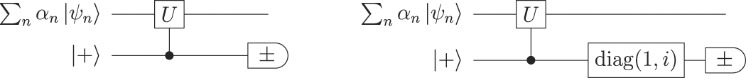
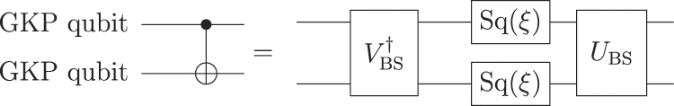
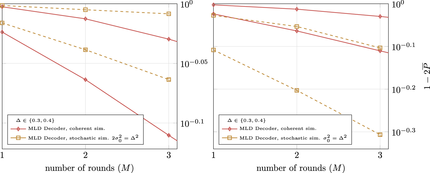
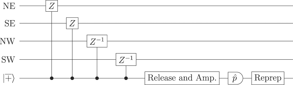