

Abstract
Robust carbon monitoring systems are needed for land managers to assess and mitigate the changing effects of ecosystem stress on western United States forests, where most aboveground carbon is stored in mountainous areas. Atmospheric carbon uptake via gross primary productivity (GPP) is an important indicator of ecosystem function and is particularly relevant to carbon monitoring systems. However, limited ground-based observations in remote areas with complex topography represent a significant challenge for tracking regional-scale GPP. Satellite observations can help bridge these monitoring gaps, but the accuracy of remote sensing methods for inferring GPP is still limited in montane evergreen needleleaf biomes, where (a) photosynthetic activity is largely decoupled from canopy structure and chlorophyll content, and (b) strong heterogeneity in phenology and atmospheric conditions is difficult to resolve in space and time. Using monthly solar-induced chlorophyll fluorescence (SIF) sampled at ∼4 km from the TROPOspheric Monitoring Instrument (TROPOMI), we show that high-resolution satellite-observed SIF followed ecological expectations of seasonal and elevational patterns of GPP across a 3000 m elevation gradient in the Sierra Nevada mountains of California. After accounting for the effects of high reflected radiance in TROPOMI SIF due to snow cover, the seasonal and elevational patterns of SIF were well correlated with GPP estimates from a machine-learning model (FLUXCOM) and a land surface model (CLM5.0-SP), outperforming other spectral vegetation indices. Differences in the seasonality of TROPOMI SIF and GPP estimates were likely attributed to misrepresentation of moisture limitation and winter photosynthetic activity in FLUXCOM and CLM5.0 respectively, as indicated by discrepancies with GPP derived from eddy covariance observations in the southern Sierra Nevada. These results suggest that satellite-observed SIF can serve as a useful diagnostic and constraint to improve upon estimates of GPP toward multiscale carbon monitoring systems in montane, evergreen conifer biomes at regional scales.
Export citation and abstract BibTeX RIS

Original content from this work may be used under the terms of the Creative Commons Attribution 4.0 license. Any further distribution of this work must maintain attribution to the author(s) and the title of the work, journal citation and DOI.
1. Introduction
Temperate forests play a critical role in the terrestrial carbon cycle, accounting for 25% of the world's forested area and 37% of the global carbon uptake (Adams et al 2019). In the coming decades, warming and drying trends are expected to continue in temperate regions, including the western United States (US) (IPCC 2023), suggesting dramatic changes to vegetation water and nutrient cycling over relatively short ecological timescales. Yet, the implications for forest carbon reserves are still unclear, particularly within heterogeneous montane environments (Rotach et al 2014), which hold the majority of aboveground biomass in the western US (Schimel et al 2002, Schimel and Braswell 2005). Higher mean temperatures and atmospheric CO2 concentrations generally enhance gross carbon uptake. However, increased water limitations may negate these effects (e.g. Angert et al 2005) while increasing the susceptibility of forests to drought-induced disturbance. This is particularly relevant in the western US mountains, where a 25% decline in total snowpack is expected by 2050, presaging a possible 'low-to-no-snow' future, which would involve critical changes to vegetation water use and physiological demands along topographic gradients (Siirila-Woodburn et al 2021). The impact on carbon cycle modeling, forest management and development along the wildland urban interface would be highly consequential, given the increasing interactions between drought, insect outbreaks and wildfires in the western US (Clark et al 2016, Fettig et al 2021).
Monitoring the forest carbon cycle is essential to understand the functional changes that accompany increasing water stress and shifting disturbance regimes. Gross primary productivity (GPP; gross photosynthetic carbon uptake by plants) represents a key monitoring indicator of ecosystem health and function. Eddy covariance (EC) towers, which measure land–atmosphere carbon exchange, are currently the most effective method for estimating GPP at the canopy scale (Baldocchi 2008), representing an average fetch of several hundred meters (Chu et al 2021). However, resource limitations have led to the spatial underrepresentation of flux measurement sites in the remote, temporally variable and heterogeneous terrain of many western US forests. Considering this and other challenges of the EC technique in complex topography, ground-based measurements alone do not constitute a sufficient regional monitoring strategy in the western US.
Satellite observations can provide more complete information at the landscape scale, particularly when used in concert with ground-based tower measurements. In remote sensing, GPP is often quantified using the light use efficiency (LUE) model (Monteith 1972):

where the photosynthetically active radiation absorbed by the plant leaf (APAR) may be estimated using ratios of surface reflectance, and the LUE of carbon assimilation is inferred empirically based on plant functional type. Traditional reflectance-based methods, such as the Normalized Difference Vegetation Index (NDVI) and the Enhanced Vegetation Index (EVI), rely on the linkage of APAR to chlorophyll content and forest canopy structure (seasonality of green leaf area) to infer GPP. However, over 90% of the forests in the western US are predominantly evergreen needleleaf forest (ENF) (Oswalt et al 2019), for which the chlorophyll content and canopy structure are seasonally invariant, rendering these models ineffective for observing temporal changes in GPP over these regions (Magney et al 2019, Pierrat et al in review).
An alternative observation method exploits a mechanistic linkage between photochemical yield and the emission of chlorophyll fluorescence, as detected by spaceborne spectrometers ('solar-induced fluorescence' (SIF)):
where  is the effective fluorescence yield, and fesc is the escape ratio of SIF from the canopy (Guanter et al
2014, Zeng et al
2019). A strong empirical relationship between SIF and GPP in ENF ecosystems has been documented from tower (Magney et al
2019) to regional scales (Frankenberg et al
2011, Walther et al
2016, Sun et al
2017, Zuromski et al
2018), where recent advances in satellite remote sensing have given way to high-resolution SIF datasets (Köhler et al
2018, Sun et al
2018). At scales of a few kilometers, satellite SIF has been shown to be insensitive to spatial variations in surface reflectance over complex surface geometries (Cheng et al
2022a), indicating a promising utility of SIF to explore spatial, seasonal and interannual patterns of photosynthesis in heterogeneous mountain terrain.
is the effective fluorescence yield, and fesc is the escape ratio of SIF from the canopy (Guanter et al
2014, Zeng et al
2019). A strong empirical relationship between SIF and GPP in ENF ecosystems has been documented from tower (Magney et al
2019) to regional scales (Frankenberg et al
2011, Walther et al
2016, Sun et al
2017, Zuromski et al
2018), where recent advances in satellite remote sensing have given way to high-resolution SIF datasets (Köhler et al
2018, Sun et al
2018). At scales of a few kilometers, satellite SIF has been shown to be insensitive to spatial variations in surface reflectance over complex surface geometries (Cheng et al
2022a), indicating a promising utility of SIF to explore spatial, seasonal and interannual patterns of photosynthesis in heterogeneous mountain terrain.
Despite strong evidence for SIF as an effective proxy for GPP, questions remain about the nature of the SIF–GPP relationship within complex terrain. Recent studies of ENF biomes have highlighted the nonuniformity of SIF–GPP scaling across seasons (Pierrat et al 2022, Yang et al 2022) and elevation-dependent land cover (Cheng et al 2022b). There is considerable debate surrounding the utility of SIF observations to detect changes in GPP due to seasonal or interannual drought (Sun et al 2015, Helm et al 2020, Marrs et al 2020, Butterfield et al 2023). For large mountain regions that span multiple climate zones and biome types, these uncertainties have yet to be investigated for their impact on regional estimates. However, understanding the limitations imposed by mountain topography on SIF–GPP relationships could better inform the scale at which biogeochemical stress indicators and disturbance precursors can be detected by satellites.
California's Sierra Nevada mountain range ('the Sierra Nevada') is an ideal domain to explore these questions, where conifer forests spanning over 3000 m in elevation have long been the focus of hydrological, biogeochemical and disturbance studies. Here, a mosaic of grass, shrub and low-density woodlands at low elevations gives way to dense, closed-canopy mixed conifer stands at mid-elevations (high leaf area index (LAI)), with reduced density near the high-elevation timberline (lower LAI) (Potter 1998, Goulden et al 2012). Sierra Nevada ecosystems exhibit summer water limitation below approximately 2000 m elevation and winter energy limitation above this elevation threshold (Trujillo et al 2012), with year-round photosynthesis occurring around the 2000 m elevation threshold, supported by deep-rooting regolith access (Kelly and Goulden 2016, O'Geen et al 2018, Rungee et al 2019). The timing of peak GPP in the Sierra Nevada has been shown to follow these patterns, ranging from spring at low elevations to mid-summer at high elevations (Goulden et al 2012, Kelly and Goulden 2016). Figure 1 synthesizes findings from past studies, summarizing the ecological expectations of GPP across seasonal and elevational gradients in the Sierra Nevada, as shaped by climatological and structural controls.
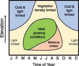
Figure 1. Expected ecological limitations to photosynthesis over elevational and seasonal gradients in the Sierra Nevada. The expectation is that the maximum photosynthetic uptake will coincide with the ideal environmental conditions in green. Patterns are informed by climate model datasets (see section 2.2) and satellite-estimated LAI and forest cover, as well as past studies of vegetation distribution (Potter 1998, Goulden et al 2012), plant water use (Trujillo et al 2012, Kelly and Goulden 2016, O'Geen et al 2018, Rungee et al 2019) and in situ EC fluxes (Goulden et al 2012, Kelly and Goulden 2016). Note that at low to mid-elevations, winter 'light limitation' is coupled with a seasonally low density of deciduous understory vegetation.
Download figure:
Standard image High-resolution imageIn this study, we evaluate the utility of high-resolution satellite-observed SIF in detecting GPP across the seasonal and elevational gradients of the Sierra Nevada. We seek to assess SIF against the ecological expectations of photosynthesis by comparing SIF with GPP from EC flux towers, a gridded model-data product (FLUXCOM) and a land surface model (CLM5.0). We discuss the limitations of SIF and GPP estimates while highlighting the advantages of SIF over other vegetation indices, presenting opportunities for the use of SIF in the carbon monitoring of montane ENFs.
2. Data and methods
A summary of the datasets and processing methods used in this study is presented in table 1. Additional information concerning the datasets and their analysis is presented as follows.
Table 1. Overview of datasets and methods used in this study.
| Data variable | Data source | Original resolution | Time range | Description | References | |
|---|---|---|---|---|---|---|
| Spatial | Temporal | |||||
| Gridded datasets | ||||||
| SIF | TROPOMI (Sentinel 5 Precursor) | 7 km × 5 km | Monthly | 2018 (February)–2021 (July) | See section 2.2. Data were oversampled from original spatial resolution to 0.04° for this study. | Köhler et al 2018, Cheng et al 2022a |
| GPP | FLUXCOM | 0.0833° | 8-daily, monthly | 2009–2020 | See section 2.2. | Jung et al 2020 |
| Elevation | NOAA/NESDIS ETOPO1 Global Relief | 1 arc second | n/a | n/a | — | Amante and Eakins 2009 |
| Land cover | European Space Agency Climate Change Initiative | 300 m | Annual | 2019 | 300 m land use categorization data from the most recent available year (2019) were quantified as 1 (ENF) or 0 (not ENF) and interpolated to 0.04° to estimate the percentage ENF coverage. The ENF domain mask was defined as grid cells with >50% ENF coverage. | Hollman et al 2013 |
| Snow cover fraction | Terra MODIS MOD10CM.061 | 0.05° | Monthly | Same as TROPOMI SIF | Snow cover was expressed as the percentage of the land surface covered by snow per grid cell. TROPOMI SIF data were omitted if the corresponding snow cover fraction was >50% due to interference from high reflected radiance. | Hall et al 2021 |
| Air temperature (daily mean) | GRIDMET | 1/24° | 3-hourly | 1980–2015 | GRIDMET temperature is derived from temporally rich meteorological data from the North American Land Data Assimilation System (NLDAS-2) and high spatial resolution from the parameter-elevation regressions on independent slopes model. | Mitchell et al 2004, Daly et al 2008, Abatzoglou 2013, Buotte et al 2019 |
| Climatic water deficit (CWD) | TerraClimate | 1/24° | Monthly | 1980–2021 | CWD is defined as the annual evaporative demand that exceeds available soil moisture (potential minus actual evapotranspiration), estimated using the Penman–Monteith approach and Thornthwaite–Mather climatic water balance model. | Abatzoglou et al 2018 |
| LAI | Terra + Aqua MODIS MCD15A2H.061 | 500 m | 8-daily | 2009–2020 | LAI is defined as the one-half total leaf surface area per unit ground area. MODIS LAI was calculated using red and near-infrared surface reflectances as well as empirical relationships of NDVI and LAI. | Myeni et al 2021 |
| Eddy covariance | ||||||
| US-CZ2 (1160 m) | Sierra Critical Zone Observatory/AmeriFlux | n/a | 30 min | 2010 (July)–2013 (January) | See section 2.3. | Data collection: Goulden 2018a, 2018b, 2018c Partitioning: Reichstein et al 2005, Wutzler et al 2018 |
| US-CZ3 (2015 m) | 2008 (September)–2016 (October) | |||||
| US-CZ4 (2700 m) | 2010 (January)–2012 (March) | |||||
| NEO-TEAK (2147 m) | National Ecological Observatory Network (NEON) | 2018 (July)–2022 (December) | Data collection: Metzger et al 2019 Partitioning: Reichstein et al 2005, Wutzler et al 2018 | |||
| Land surface model | ||||||
| GPP (regional) | Community Land Model 5.0 | 1.96° × 1° | Daily | 1980–2015 | GPP was simulated under two separate configurations: CLM5.0 with biogeochemistry (CLM5.0-BGC) and CLM5.0 with prescribed leaf and stem area from the MODIS satellite data (CLM5.0-SP). The full model setup is detailed in appendix C. | Lawrence et al 2019, Danabasoglu et al 2020, Raczka et al 2021 |
| GPP (site level) | n/a | Daily | Site-specific land cover, forest canopy cover and bedrock depth were defined using the AmeriFlux Biological, Ancillary, Disturbance, and Metadata files | https://ameriflux.lbl.gov/data/badm/ | ||
a Notes: Gridded datasets were re-rasterized from their original resolution to match the spatial resolution of TROPOMI SIF used in this analysis (0.04°). b The time range for US-CZ2 (1160 m) flux data was abbreviated from 2010 to 2013 to account for the effects of disturbance on mean seasonality at the site (see appendix B).
2.1. Sierra Nevada study domain and land cover
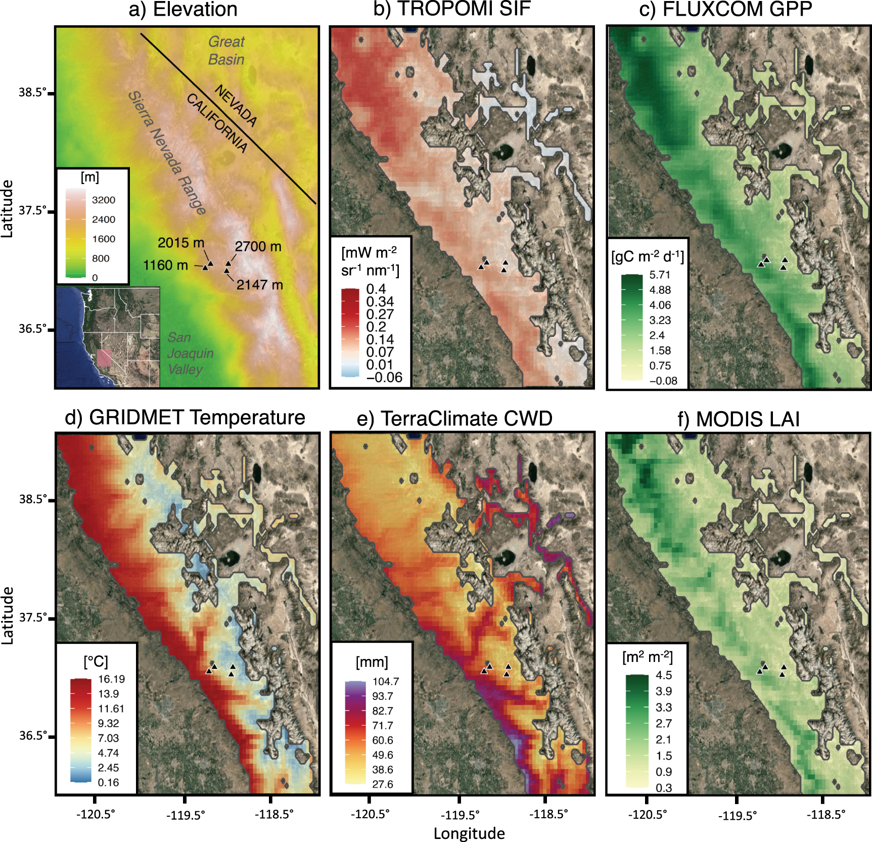
Our study domain encompassed 28 700 km2 of ENF within California's Central and Southern Sierra Nevada, covering an altitudinal gradient ranging from 300 to 3400 m above sea level (NOAA ETOPO1 elevation model shown in figure 2(a)). The climate is montane Mediterranean; most annual precipitation falls during winter when rain–snow transitions are around 2000–2500 m in elevation (Shulgina et al 2023). The European Space Agency's (ESA) Climate Change Initiative land cover dataset (Hollman et al 2013) was used to define the ENF domain boundaries; areas of other prevailing land cover types were omitted from this analysis (see table 1).
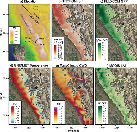
Figure 2. Gridded time-averaged datasets over the Sierra Nevada domain, filtered for evergreen forest mask. (a) elevation, (b) mean annual TROPOMI SIF, (c) mean annual FLUXCOM GPP, (d) mean annual GRIDMET temperature, (e) mean annual TerraClimate CWD (i.e. potential minus actual evapotranspiration) and (f) peak season (July) MODIS LAI. Flux tower sites are represented as black triangles and labeled by elevation in panel (a). Panels (b), (c) and (f) are filtered for 2018–2020 when the availability of TROPOMI SIF, FLUXCOM GPP and MODIS LAI overlap.
Download figure:
Standard image High-resolution image2.2. Gridded SIF, GPP, modeled climate and vegetation indices
Individual SIF retrievals from TROPOMI (the single payload of the ESA Sentinel-5 Precursor satellite) soundings were gridded to a monthly time resolution and 0.04° spatial resolution, which oversampled the native 7 × 5 km resolution. Instantaneous SIF values at 740 nm were scaled to daily mean values (often denoted as SIFdc but herein denoted as SIF for simplicity), as described by Köhler et al (2018). The SIF data were further corrected to account for the effects of surface geometry on solar incidence angle (Cheng et al 2022a), which are minimal on average (3% mean difference over domain) but can reach up to 92% for some grid cells in the winter months. To minimize noise from high reflected radiance over snowy surfaces, we used MODIS monthly snow cover (MOD10CM) to filter out pixels with high snow cover. The spatial pattern of the mean annual SIF over the region is shown in figure 2(b). To match the grid resolution of TROPOMI SIF, all other gridded data in this study were re-gridded to 0.04° resolution via bilinear interpolation, resulting in a negligible impact on seasonal and elevation patterns across the domain.
We used monthly gridded estimates of GPP from the FLUXCOM-RS ensemble remote-sensing carbon flux product ('FLUXCOM'; Jung et al 2020), distributed natively at 1/12° (∼0.0833°) resolution. FLUXCOM is the median of 18 ensemble members, where nine machine-learning methods were used to predict two flux-partitioning variants for GPP. The models were trained using 8-daily MODIS vegetation and moisture reflectance indices along with land surface temperature and radiation as input, as well as data from >200 FLUXNET EC towers (Tramontana et al 2016, Pastorello et al 2020), excluding the Sierra Nevada sites used in this study.
Daily mean temperature and CWD (defined as reference evapotranspiration minus actual evapotranspiration) were estimated using the GRIDMET and TerraClimate models (Abatzoglou 2013, Abatzoglou et al 2018) to serve as additional diagnostics for the temperature and moisture limitations of GPP.
We compared the patterns of SIF and GPP to those of five spectral reflectance-based vegetation indices (NDVI, kNDVI, EVI, EVI2 and near-infrared reflectance of vegetation (NIRv)) from the MODIS satellite instrument. Details of these comparisons and the datasets used are summarized in appendix A.
2.3. EC flux tower data
EC measurements of net ecosystem exchange (NEE) were taken along with meteorological data from four flux towers along an elevational gradient in the southern Sierra Nevada. These include the AmeriFlux sites US-CZ2 (1160 m), US-CZ3 (2015 m) and US-CZ4 (2700 m), and the National Ecological Observatory Network's (NEON) TEAK site (2147 m) (table 1 and figure 2(a)).
NEE data were filtered to remove calm periods and then gap-filled using the REddyProc package version 1.3.2 in R (Wutzler et al 2018). Ecosystem respiration (Reco) was estimated by fitting a temperature sensitivity function from the gap-filled nighttime NEE (Reichstein et al 2005) following procedures described by Wutzler et al (2018). The half-hourly estimated Reco was subtracted from NEE to obtain GPP and aggregated to monthly timescales to match the timing of TROPOMI. Mismatch between spatial scales of the EC observations (footprint <1 km2) and gridded data (∼16 km2 pixels) is an inherent limitation in heterogeneous terrains (see section 4.3). We specifically accounted for the effects of a localized disturbance event within the 1160 m EC tower footprint by filtering the site's data for time periods when the canopy structure (indicated by MODIS NIRv) was aligned between the flux tower footprint and TROPOMI grid cell footprint scales. A full description of this methodology is presented in appendix B.
2.4. Land surface model
The Community Land Model 5.0 (CLM5.0; Lawrence et al 2019) was used to simulate GPP to serve as both a validation and diagnostic tool for TROPOMI SIF. Simulations were run using two different modules of CLM5.0, one with a prognostic vegetation state and active biogeochemistry (CLM5.0-BGC), and the other with satellite-prescribed phenology from MODIS LAI data (CLM5.0-SP). In this study, regional simulations were forced by GRIDMET meteorology following Raczka et al (2021) and centered on the Sierra Nevada domain along with site-level simulations at the four flux tower locations described in section 2.3. The model setup is summarized in table 1; configuration and diagnostic analyses are detailed in appendix C.
2.5. Statistical methods
To compare seasonal trends between datasets, we computed the mean seasonal cycle of monthly SIF and GPP as the average across all years specific to each dataset (see table 1). Flux tower GPP was compared against CLM5.0 point simulations as well as gridded TROPOMI SIF and FLUXCOM GPP extracted over the flux tower locations. GPP estimates were averaged monthly to match the monthly SIF observations. We computed the difference in the timing of the peak EC GPP with that of the peak TROPOMI SIF (tEC_peak − tSIF_peak) and FLUXCOM and CLM5.0 GPP (tEC_peak − tGPP_peak), including both CLM-BGC and -SP model configurations. A positive (negative) difference indicates that the EC peak occurred later (earlier) than the comparison dataset.
To assess the synchronicity of the seasonal patterns in SIF and GPP, we performed cross-correlation analyses to obtain the time-lag shift (in months) of the maximum correlation between cycles at each flux tower site (denoted as tEC_cycle − tSIF_cycle for TROPOMI and tEC_cycle − tGPP_cycle for FLUXCOM and CLM5.0). SIF was compared with EC GPP by expressing both quantities as fractions relative to their respective maxima across sites. The coefficient of determination (R2) was computed for each cycle comparison after applying the time lag.
Seasonal and elevational trends were determined by aggregating monthly average gridded SIF, GPP and climatology datasets into 100 m elevation bins from the elevation model to represent the average gridded value for that elevation band. We also computed the domain-aggregated relative distribution across elevation or season by averaging all gridded SIF and GPPs in elevation (or time), calculating the rolling average using a 100 m (or 2 week) window and dividing by the maximum window-mean value.
3. Results
3.1. Seasonal and elevational patterns of gridded SIF and GPP
The annual mean distributions of TROPOMI SIF and FLUXCOM GPP (figures 2(b) and (c)) followed similar spatial patterns throughout the Sierra Nevada, both resembling the spatial pattern of MODIS LAI (figure 2(f)). The majority of SIF and GPP activity was located in the northern third of the domain (38°–39° N, figures 2(b) and (c)), where elevations are mostly below 2000 m and LAI is high.
Seasonal and elevational trends of SIF and GPP are shown in figures 3(a)–(d), and trends of temperature and CWD are shown in figures 3(e) and (f). The peak TROPOMI SIF occurred in June at mid-elevations (1000–1500 m), with a smaller April peak at low elevations influenced by the spring growth of herbs, grasses and deciduous shrubs. SIF consistently decreased with elevation above these peak zones and decreased from early summer to fall and winter across all elevations. Tracing the elevation and timing of the 90th percentile range of SIF to the GRIDMET temperature (figure 3(e)) gave a corresponding daily mean range of 18 °C–19 °C for the June peak.
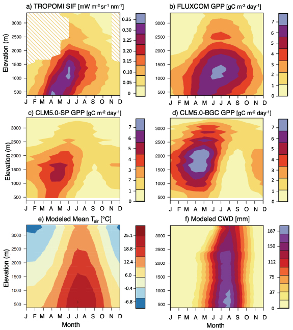
Figure 3. Patterns of gridded datasets and model output over elevation and mean seasonality for (a) TROPOMI SIF, (b) FLUXCOM GPP, (c) simulated CLM5.0-SP GPP, (d) simulated CLM5.0-BGC GPP, (e) GRIDMET model mean temperature and (f) TerraClimate modeled CWD (reference ET—actual ET).
Download figure:
Standard image High-resolution imageElevational trends of FLUXCOM GPP resembled those of TROPOMI SIF, with a maximum around 1300–1500 m; however, FLUXCOM GPP peaked slightly later than SIF (June–July) and remained high throughout the summer (figure 3(b)). The GRIDMET temperature corresponding to the 90th percentile of FLUXCOM GPP ranged from 17 °C to 24 °C, which is considerably warmer than the corresponding temperature range for TROPOMI SIF's 90th percentile. Below 750 m, seasonal GPP was reduced after May (similar to TROPOMI); however, FLUXCOM GPP showed more sustained patterns throughout the summer than SIF, extending significant GPP through September at mid-elevations.
CLM5.0-SP simulations also exhibited seasonal and elevational GPP patterns similar to those of FLUXCOM and TROPOMI SIF (figure 3(c)), whereas CLM5.0-BGC simulations differed significantly in magnitude and elevational patterns (figure 3(d)). The CLM5.0-SP peak GPP was lower in magnitude than FLUXCOM GPP, occurring earlier (April–May) but at a similar elevation range (1200–1700 m). CLM5.0-BGC showed a strong, early seasonal GPP peak around March–May at a high elevation band around 1500–2000 m, concomitant with strong, high-elevation patterns in the model LAI (see appendix C). The corresponding mean GRIDMET temperature at the 90th percentile model GPP ranged from 7 °C to 14 °C for CLM5.0-SP and from 4 °C to 12 °C for CLM5.0-BGC. For both BGC and SP simulations, the peak GPP was slightly delayed with increasing elevation. This was followed by an extensive dormant period from July through November, concurrent with seasonally low soil moisture (appendix C).
3.2. SIF and GPP averaged across time and elevation
Averaging gridded datasets across time allowed us to explore the general relationship between SIF and GPP products and elevation within the Sierra Nevada. TROPOMI SIF and FLUXCOM GPP exhibited similar elevational distributions, with most SIF and GPP (above a relative distribution threshold of 80%) distributed between 700 and 1700 m (figure 4(a)). This 80% relative distribution threshold occurred slightly higher for MODIS LAI and CLM5.0-SP GPP, between 800 and 2200 m and 900 and 2400 m elevations, respectively. CLM5.0-BGC GPP was allocated substantially higher in elevation (>80% relative distribution between 1700 and 2700 m), reflecting the impact of prognostic LAI (CLM5.0-BGC) vs. satellite-prescribed LAI (CLM5.0-SP) upon simulated GPP (see appendix C).
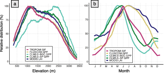
Figure 4. (a) Elevational patterns of annual mean TROPOMI SIF (red), FLUXCOM GPP (yellow), simulated GPP from CLM5.0-BGC (light green), CLM5.0-SP (dark green) and MODIS LAI (navy), separated by elevation bin and expressed as a percentage of the maximum signal over a 100 m moving elevation window. (b) Mean seasonal cycle of spatially aggregated TROPOMI SIF, FLUXCOM GPP, simulated GPP from CLM5.0-BGC, CLM5.0-SP and MODIS LAI (same color scheme as panel (a)), over the full Sierra Nevada domain extent, expressed as a percentage of the maximum signal over a 2 week moving time window.
Download figure:
Standard image High-resolution imageAveraged across space, we observed key differences in the seasonality of the datasets (figure 4(b)). Both CLM simulations exhibited a spring increase from January to mid-April, approximately 1.5 months earlier than TROPOMI SIF and FLUXCOM GPP, which increased in near synchrony from mid-February to June. CLM5.0-SP and CLM5.0-BGC GPP declined in response to moisture limitation from May and June, respectively, until both reached seasonal minimums in September and increased again in fall to winter. The domain-averaged TROPOMI SIF peaked sharply in June and then decreased steadily to a seasonal minimum in December. FLUXCOM timing was closely tied to MODIS vegetation indices (figure A2) and diverged from the patterns of SIF and CLM GPP. Both FLUXCOM GPP and LAI were sustained above 75% of the maximum through October and declined toward seasonal minimums in winter, depicting a nearly 2.5 months longer growing season in FLUXCOM GPP than in TROPOMI SIF. Additional MODIS vegetation indices showed little seasonal variation relative to SIF and GPP estimates (figure A2).
3.3. Site-level observations vs. SIF and GPP products
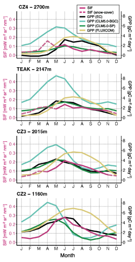
Figure 5 shows the mean seasonal cycle of GPP from the four EC sites compared with gridded SIF, FLUXCOM GPP and CLM5.0 point simulations. Among the models, CLM5.0-SP provided the best match to the seasonal timing and magnitude of EC GPP, whereas CLM5.0-BGC consistently overestimated EC GPP. Both CLM model configurations inadequately captured winter dormancy at the higher elevation sites (2147 and 2700 m) between November and March. Both CLM configurations also showed more dramatic reductions in summer GPP at lower elevations, resulting from seasonal water limitation. FLUXCOM better captured winter dormancy at high elevation sites compared to CLM simulations; however, it showed a positive bias compared to flux towers during summer and fall, particularly at lower elevations. SIF mainly followed the relative patterns of EC GPP; it did not capture winter dormancy at 2147 and 2700 m, but we assumed this to be caused by reflected radiance and thus omitted SIF during periods of snow cover (dashed line). SIF was also low relative to EC GPP at 2700 m because of 'dilution' from the non-vegetated terrain within this pixel.
Figure 5. Comparison of mean seasonal cycles: TROPOMI SIF (red), EC GPP (black), modeled GPP from CLM5.0-BGC (light green), CLM5.0-SP (dark green) and FLUXCOM GPP (yellow). Comparisons are shown at each of the four flux tower sites along the Sierra Nevada elevational transect. SIF is shown in dashed lines, where the mean MODIS snow cover fraction was over 50%, to denote periods where SIF was omitted from the analysis due to noise from high reflected radiance. All seasonal cycles represent the multi-year average across their respective available time ranges listed in table 1.
Download figure:
Standard image High-resolution image
Time series analyses are summarized in table 2, showing lags in the timing of peak signals, as well as the seasonally integrated cross-correlation lags between full seasonal cycles. TROPOMI SIF was consistently within 1 month of EC GPP, considering both peak timing and full seasonal cross correlation. (Lag R2 values were low at high elevation sites due to lower SIF sample size from snow cover filtering in winter and spring.) The modeled GPP from CLM5.0-SP was also consistently within 1 month of EC GPP. FLUXCOM GPP timing was close to that of EC GPP at high elevation sites but was up to 2 months delayed from EC GPP at lower elevations. CLM5.0-BGC was the least synchronous with EC GPP timing, often 2 months offset from ground-based estimates.
Table 2. Results of timing analyses of multi-year mean seasonal cycles. tEC_peak − tSIF_peak and tEC_peak − tGPP_peak are the differences (in months) between peak EC GPP and peak TROPOMI SIF, FLUXCOM GPP or CLM5.0 GPP. tEC_cycle − tSIF_cycle and tEC_cycle − tGPP_cycle are the lag differences (in months) from cross-correlation analyses, where the lag shown is the timing shift at which EC and SIF, FLUXCOM or CLM5.0 achieve maximum correlation. Lag R2 values are the coefficients of determination from the cross-correlation function. For all timing differences, negative values indicate that the signal (SIF, FLUXCOM or CLM5) is delayed from the EC GPP cycle; positive values indicate that the signal is ahead of the EC GPP cycle.
| Site name | Elevation (m) | TROPOMI SIF | FLUXCOM GPP | CLM5.0-BGC GPP | CLM5.0-SP GPP | ||||||||
|---|---|---|---|---|---|---|---|---|---|---|---|---|---|
| tEC_peak − tSIF_peak (months) | tEC_cycle − tSIF_cycle (months) | Lag R2 | tEC_peak − tGPP_peak (months) | tEC_cycle − tGPP_cycle (months) | Lag R2 | tEC_peak − tGPP_peak (months) | tEC_cycle − tGPP_cycle (months) | Lag R2 | tEC_peak − tGPP_peak (months) | tEC_cycle − tGPP_cycle (months) | Lag R2 | ||
| US-CZ4 | 2700 | 0 | 1 | 0.45 | 0 | 1 | 0.89 | 1 | 2 | 0.75 | 0 | 1 | 0.83 |
| TEAK | 2147 | −1 | 0 | 0.56 | −1 | 0 | 0.91 | 0 | 1 | 0.84 | −1 | 0 | 0.94 |
| US-CZ3 | 2015 | −1 | −1 | 0.76 | −2 | −1 | 0.77 | 0 | 0 | 0.84 | 0 | 0 | 0.88 |
| US-CZ2 | 1160 | 0 | 0 | 0.81 | 0 | −1 | 0.84 | 2 | 2 | 0.77 | 1 | 1 | 0.74 |
4. Discussion
4.1. Patterns of GPP and SIF compared to expected limitations
The elevational and seasonal trends of TROPOMI SIF, FLUXCOM GPP and CLM5.0-SP (figures 3(a–c)) largely align with the ecological expectations for environmental limitations on GPP described in figure 1 and in the climate and land cover datasets used here.
4.1.1. Temperature limitation
The daily mean winter temperature threshold for strong cold limitation along the Sierra Nevada flux tower transect is likely somewhere between 2.5 °C (winter-dormant 2700 m site) and 6.3 °C (winter-active 2015 m site) (Goulden et al 2012). This occurs between 1500 and 2000 m elevation in December–January according to the GRIDMET modeled temperature across the Sierra Nevada study region (figure 3(e)). Both CLM5.0-SP and FLUXCOM GPP suggest a significant transition between 1500 and 2000 m in winter, with negligible GPP above 2000 m from December to March (figure 3(b)), following Goulden et al (2012). In contrast, the modeled GPP from CLM5.0-BGC showed virtually no winter dormancy, except above 3000 m. Although wintertime SIF could not be effectively analyzed due to snow contamination, these results demonstrate consistency between gridded GPP and the existing literature for winter patterns in the Sierra Nevada.
During summer, the 90th percentile of gridded SIF corresponds to the GRIDMET mean air temperature (18 °C–19 °C) near or within the optimal temperature range reported in global synthesis studies (∼15 °C–20 °C per Duffy et al (2021), 18 °C–20 °C for ENF per Chen et al (2023), and ∼13 °C–17 °C for ENF per Huang et al (2019)). The 90th percentile of FLUXCOM GPP corresponds to a much higher temperature range (17 °C–24 °C) than in these studies, suggesting that the peak growing season in FLUXCOM is biased late into the hot summer. Conversely, the peak modeled GPP from CLM5.0 occurs at cooler elevations and months (7 °C–14 °C for SP and 4 °C–12 °C for BGC), which we attribute to a slight early-season bias in CLM5.0-SP and an early-season high-elevation bias for CLM5.0-BGC linked to patterns in simulated LAI.
4.1.2. Moisture limitation
TerraClimate-modeled CWD is strongly seasonal and greatest in late summer (figure 3(f)); however, patterns in CWD are not necessarily consistent with observations, given that numerous studies (Goulden et al 2012, Kelly and Goulden 2016, O'Geen et al 2018, Rungee et al 2019) have observed the capacity of the mid-elevation Sierra Nevada forests to maintain GPP and ET throughout the summer. This is because roots can reach at least 5 m deep (Kelly and Goulden 2016), allowing consistent access to subsurface water storage.
Our findings suggest that moisture limitation may still have an impact on seasonal GPP in the Sierra Nevada, depending on the elevation. A distinct late-season bias in FLUXCOM is apparent compared to flux tower GPP at low to mid-elevations (figure 5, table 2) and compared to SIF and modeled GPP (figure 4(b)), which we suspect is caused by the underestimation of water stress effects in FLUXCOM. Conversely, CLM5.0-SP generally matches EC GPP timing (figure 5) and is well constrained by moisture limitation, particularly between 1000 and 2000 m (appendix C). The lowest site (1160 m) is an exception, with higher seasonal EC GPP compared to CLM5.0-SP, suggesting a balance between seasonal drought and deep subsurface water access. Although CLM5.0 represents both rooting depth and subsurface hydrology, it does not represent deep roots (>1 m) that have access to water. SIF, on the other hand, most closely matches EC GPP timing at 1160 m, indicating that SIF may indeed capture seasonal moisture limitation.
4.1.3. Vegetation density limitation
Above the mid-elevation range (∼1500 m), we expect vegetation density to be a major limitation to GPP during peak growing season, noting a relatively consistent LAI gradient of −1.1 (−38%) per kilometer in elevation. The elevational gradients of TROPOMI SIF, FLUXCOM GPP and CLM5.0-SP scale proportionally to LAI in July at −40%, −33% and −43% per kilometer, respectively. The model-simulated LAI in CLM5.0-BGC caused unrealistically high GPP at high elevations, diverging substantially from the expected vegetation density-driven elevational patterns. Unlike the other models, CLM5.0-BGC was not calibrated with LAI observations for the Sierra Nevada mountain range. Thus, we did not expect CLM-BGC to perform as well. Flux tower GPP has a slightly milder elevational gradient in July (−28% per kilometer elevation from 1160 to 2700 m sites), although we speculate that the 2700 m EC site likely exhibits higher LAI than average for that elevation due to its selection as a forest EC site. Overall, there is a strong similarity between the elevational gradients of LAI, SIF and GPP during the peak growing season, aligning with expectations (figure 1).
4.2. Comparison of mean seasonal cycles
The timing of the spring onset and June–July peak of TROPOMI SIF and FLUXCOM GPP (figure 4(b)) agree with previous studies of ENF GPP in the Sierra Nevada (Goldstein et al 2000, Misson et al 2006, Goulden et al 2012). Our findings of TROPOMI SIF seasonality are similar to the results of Turner et al (2020) across California, which showed peak TROPOMI SIF from ENF between June and July. FLUXCOM GPP seasonality generally matched other FLUXCOM studies (Byrne et al 2018 (ENF); Sun et al 2018), although the FLUXCOM GPP shown here is comparatively high in fall. The most significant deviation between TROPOMI SIF and FLUXCOM occurred after the initial peak in June (figure 4(b)), when SIF declined sharply and FLUXCOM GPP remained high throughout the summer and into the fall, during which we would expect water stress to limit GPP to some extent (section 4.1). Similar seasonal deviations between TROPOMI SIF and FLUXCOM GPP have been documented (e.g. Chen et al 2021b). We suspect that these deviations reflect the strong coupling of FLUXCOM GPP to MODIS vegetation indices (NDVI, EVI, NIRv, etc) during summer and early fall (figure A2). However, TROPOMI SIF captured the expected seasonal downregulation of photosynthesis much more effectively than the other satellite-based vegetation indices. As a result, the seasonal and elevational patterns of TROPOMI SIF and FLUXCOM GPP were more highly correlated than any other gridded GPP comparison, including comparisons with NIRv, EVI, NDVI, etc (see appendix A).
In theory, flux tower observations should serve to further connect these global gridded datasets to local patterns of GPP. The mean seasonalities of TROPOMI SIF and CLM5.0-SP were both consistently within 1 month of the mean EC GPP seasonality, whereas the mean seasonality of FLUXCOM GPP was consistently delayed from EC GPP. This helps explain the significant summer–fall deviations between the TROPOMI and FLUXCOM signals, providing more confidence that TROPOMI SIF appropriately tracks the timing of GPP across the Sierra Nevada elevational gradient.
4.3. Limitations and applications to carbon monitoring systems
Functional carbon monitoring systems across the western US will need to rely on robust connections between ground- and satellite-based data over complex terrain. In addition to SIF, other remote-sensing and ground-based data streams will help further elucidate biophysical (e.g. NDVI and NIRv), biochemical (e.g. photochemical reflectance index (Gamon et al 1997) and chlorophyll/carotenoid index (Gamon et al 2016)) and hydrologic (e.g. soil moisture and snow cover) processes. Nonetheless, there is burgeoning scientific interest in satellite-based SIF for carbon monitoring and early stress detection, so far mostly in agricultural systems (Zhang et al 2019, 2023, Peng et al 2020, Sloat et al 2021, Mohammadi et al 2022). A growing body of evidence points toward the linearity of the SIF–GPP relationship at seasonal canopy scales (Frankenberg et al 2011, Yang et al 2015, Li and Xiao 2019, Magney et al 2020). Future research is needed to determine how the time series of SIF over ENF biomes correlate with carbon fluxes over ecologically meaningful timescales (years to decades). To this end, several limitations are important to consider.
4.3.1. SIF and land cover
The relatively low signal-to-noise ratio of satellite-based SIF will remain a limitation, requiring averaging in space and/or time to increase precision. We found that snow cover was a large source of noise in the satellite SIF, introducing a large positive bias into the SIF signal. Highly reflective and heterogeneous land cover also has strong effects on signal-to-noise SIF ratios (Köhler et al 2018, Cheng et al 2022b). High-resolution land cover and disturbance datasets will be useful to help identify and separate these influences from overall biome trends, but users must be aware of the sub-grid scale heterogeneity and classification uncertainty. One must also consider the changing seasonal role of environmental drivers (snow, soil moisture, heat and APAR), which have been shown to have asymmetric impacts on the SIF–GPP relationship even at the satellite scale (Chen et al 2021a).
4.3.2. GPP
Model-data estimates of GPP (e.g. FLUXCOM) are useful for areas without significant EC data coverage. However, one must consider the impact of extrapolation of these estimates to under-sampled heterogeneous terrain. It is also important to consider that analyses of EC GPP in heterogeneous terrain are ultimately influenced by site selection, as well as the averaging period and grid resolution of the comparison datasets. For example, the EC data at the 1160 m site were significantly impacted by drought-induced disturbance from 2013 to the present (Goulden and Bales 2019, appendix B). However, typical EC footprints are small relative to many satellite data scales (e.g. <5% of the original TROPOMI sampling area). Thus, disturbances may be impactful at the EC scale but negligible at the satellite scale, or vice versa. This exemplifies the challenges in tower-satellite representation, which are well described in other vegetation remote-sensing studies (e.g. Yu and Ma 2015, Lu et al 2018, Schimel and Schneider 2019, Du et al 2023), particularly those within complex terrain (Desai et al 2011).
4.3.3. Terrestrial biosphere models
Fully prognostic land surface models, such as CLM-BGC, have well-documented shortcomings in capturing vegetation phenology (e.g. mischaracterized rooting depth and uncaptured winter dormancy; Richardson et al 2012, Raczka et al 2016, 2019), which, to some extent, we have addressed here through the prescription of LAI observations into CLM5-SP. In general, systematic biases in land surface models due to deficiencies in process representation cannot be fully addressed through the implementation of fine-scale land surface and atmospheric forcing data alone (Duarte et al 2022). Future work intends to utilize model-data fusion techniques, such as ensemble data assimilation (Raczka et al 2021), to leverage satellite observations (SIF, leaf area and snow cover) and recent canopy-level SIF representation in CLM (Li et al 2022).
5. Conclusion
Satellite remote sensing of vegetation will be integral to the development of carbon flux monitoring systems, both globally and regionally, with montane evergreen conifer forests in the western US presenting unique challenges to monitoring goals at these scales. Here, we assessed the ability of high-resolution satellite SIF to track the average trends of photosynthesis across seasons and elevations in one of the largest and most dynamic mountain ranges in the western US. After filtering for snow-covered surfaces, TROPOMI SIF showed strong agreement in elevational patterns with a robust model-data GPP product (FLUXCOM) and a data-constrained land surface model (CLM5.0-SP) while closely matching the mean seasonal timing of EC tower GPP across four flux monitoring sites in the Sierra Nevada. We also found that, compared to active biogeochemistry (CLM5.0-BGC) simulations, modeled GPP constrained by satellite phenology (CLM5.0-SP) showed substantially better agreement with EC GPP. The spatial mismatch between EC and gridded satellite data, combined with localized disturbance events, presents challenges for tower-to-satellite-scale comparisons. Nonetheless, SIF and FLUXCOM GPP were more highly correlated across elevations and seasons than any other combination of gridded GPP and satellite vegetation indices. These findings provide strong evidence that satellite-based SIF can provide unique and valuable information to carbon monitoring systems over mountainous ENF regions, such as the western US, particularly when integrated with data assimilation techniques.
Acknowledgments
This research was funded by the NASA Carbon Monitoring Systems program Award 80NSSC20K0010 and the National Science Foundation Graduate Research Fellowship Program Award #2139322. Additional funding was provided by the US National Science Foundation Macrosystems Biology and NEON-Enabled Science (Award 1926090) and Division of Environmental Biology (Award 1929709) programs.
Data availability statements
The eddy covariance data were provided by the AmeriFlux Network and the National Ecological Observatory Network (NEON). NEON is a program sponsored by the National Science Foundation and operated under the cooperative agreement of Battelle. This material is based in part on work supported by the National Science Foundation through the NEON program.
The data that support the findings of this study are openly available at the following URL/DOI: https://doi.org/10.5281/zenodo.8239702.
Conflict of interest
The authors have no competing interests to declare.
Appendices (1.0 MB PDF) Appendix A: Comparisons with vegetation indices. Appendix B: Omission of mortality event from EC flux data using MODIS NIRv. Appendix C: CLM5 setup and diagnostic analyses."