

Abstract
As an important carbon sink to mitigate global climate change, the role of arid and semiarid grassland ecosystem has been widely reported. Precipitation and temperature changes have a dramatic impact on the carbon balance. However, the study of wind speed has long been neglected. Intuitively, wind speed regulates the carbon balance of grassland ecosystems by affecting the opening of vegetation stomata as well as near-surface moisture and temperature. It is sufficient that there is a need to conduct field observations to explore the effect of wind speed on the carbon balance in arid and semiarid grassland. Therefore, we conducted observations of carbon fluxes and corresponding climate factors using an eddy covariance system in a typical steppe in Inner Mongolia from 2017 to 2021. The research contents include that, (i) we depicted the changing patterns of carbon fluxes and climate factors at multiple time scales; (ii) we simulated the net ecosystem carbon balance (NECB) based rectangular hyperbolic model and compared it with the observed net ecosystem exchange values; (iii) we quantified the mediated effect of wind speed on NECB by adopting structural equation modeling; (iv) we used the constrained line method to explore what wind speed intervals might have the greatest carbon sequestration capacity of vegetation. The results were as follows, (i) the values of NECB for the five years of the study period were 101.95, −48.21, −52.57, −67.78, and −30.00 g C m−2 yr−1, respectively; (ii) if we exclude the inorganic carbon component of the ecosystem, we would underestimate the annual carbon balance by 41.25, 2.36, 20.59, 22.06 and 43.94 g C m−2 yr−1; (iii) the daytime wind speed during the growing season mainly influenced the NECB of the ecosystem by regulating soil temperature and vapor pressure deficit, with a contribution rate as high as 0.41; (iv) the grassland ecosystem had the most robust carbon sequestration capacity of 4.75 μmol m−2 s−1 when the wind speed was 2–3 m s−1. This study demonstrated the significant implications of wind speed variations on grassland ecosystems.
Export citation and abstract BibTeX RIS

Original content from this work may be used under the terms of the Creative Commons Attribution 4.0 license. Any further distribution of this work must maintain attribution to the author(s) and the title of the work, journal citation and DOI.
1. Introduction
Grasslands, accounting for 1/5 of the global land area and 41.1% of China's national territory, are mainly distributed in arid and semiarid zones (Akiyama et al 2007, Mu et al 2013, Pan et al 2018) and are not only essential carbon pools in the carbon cycle of terrestrial ecosystems but also have a significant impact on the atmospheric GHG content (Leahy et al 2004, Maia et al 2009, Henderson et al 2015, Yang et al 2019). Grassland ecosystems are the largest carbon pool in terrestrial ecosystems except for forest ecosystems, and their carbon stocks are equal to approximately 1/3 of terrestrial ecosystems, most of which exist in soil as organic carbon (Hungate et al 1997, Scurlock et al 2002, Tang et al 2018). For the carbon pool of grassland ecosystems in China, the total carbon pool is approximately 29.1 Pg C, of which the soil carbon pool accounts for more than 96% of the total (Piao et al 2009, Fang et al 2010). In addition to sequestering carbon in terrestrial carbon pools and natural climate solutions to reduce greenhouse gas emissions, grassland restoration is one of the critical measures for reducing greenhouse gas emissions from 2000 to 2020 (Griscom et al 2017). The total additional (maximum additional mitigation potential) MAMP of grassland ecosystems is projected to be at least 68–82 Tg CO2 yr−1 during 2020–2060 (Lu et al 2022).
Significant amounts of inorganic carbonates were found in the soils of these ecosystems, which can be crucial to determining a net ecosystem carbon balance (NECB), an indicator of the amount of carbon that an ecosystem accumulates in a given period, which is based on both biological and physical processes (Chapin et al 2006, Smith et al 2010). There are important differences between NECB and net ecosystem exchange (NEE) related to the entry and exit of inorganic carbon, as well as when other nonbiogenic sources of carbon enter or leave the ecosystem (Wohlfahr et al 2012). The contribution of inorganic carbon is small when estimating NECB on an annual scale (Hirmas et al 2010, Liu et al 2020). Weathering of carbonates and erosion by precipitation occurred in a relatively short period of time during different periods, which can affect the NECB on a daily basis (Lal 2019, Abbott 2022). Therefore, semiarid ecosystems are essential not only for understanding how carbon and energy exchange takes place and their importance on a global level but also for their potential to reveal an array of other exchanges pertinent to the global scale that have not been adequately understood or considered. Therefore, inorganic carbon must also be considered in the NECB of these ecosystems.
In light of the fact that arid and semiarid ecosystems are prone to experiencing greater variations in precipitation and temperature than other ecosystems (Fensholt et al 2012, Nielsen et al 2015, Jiang et al 2020, Li et al 2021). Due to the intricate influence of various factors on temperature and precipitation, the resulting uncertainty demands a comprehensive understanding of the process of carbon balance change to accurately quantify the contribution of each individual factor (Aragão et al 2014, Müller et al 2016). In recent years, a large number of scholars have begun to study the effects of wind speed changes on grassland ecosystems, mainly focusing on the following aspects and drawing relevant conclusions: (1) wind speed affects plant growth rate and leaf morphology. Optimal wind speed facilitates plant growth, development, and enhanced primary productivity of vegetation. Conversely, excessive or prolonged wind conditions exert detrimental effects on plant vitality, impeding growth and development (Van Gardingen and Grace 1991, Cleugh et al 1998); (2) wind will be the first to carry away fine particles from the surface soil, which will lead to coarsening of soil texture, decrease of moisture and redistribution of nutrients (De Langre 2008, Colazo and Buschiazzo 2015); (3) wind causes the transfer and exchange of materials and energy between the surface boundary layer and the atmospheric boundary layer, and the exchange of heat and water vapor leads to changes in the surface microclimate, such as a decrease in wind speed, which leads to an increase in surface temperature (Armstrong et al 2014); (4) the wind effect makes soil water deficit and nutrient composition change, which leads to the change of grassland ecosystem structure, decrease of grassland cover, complication of species life type, and increase of drought-tolerant plants (Saxton et al 2006); (5) the exchange rate of CO2 increases with increasing wind speed, and the same applies to carbon emissions (Montaldo et al 2013). It has been discussed in studies at the regional scale that widespread decline in winds delayed autumn foliar senescence over high latitudes; wind was the primary driver of carbon balance in Spanish semiarid grassland ecosystems (Rey et al 2012, Wu et al 2021, Zhang et al 2022). However, the role of wind speed in regulating the carbon balance of grassland ecosystems throughout the year has not been considered.
This study examined the mechanisms that regulate the exchange of carbon, water, and heat between the atmosphere and a semiarid grassland of the Inner Mongolia Plateau, Northern China, over a period of five consecutive years. The specific aims were (1) to quantify the potential contribution of grass steppes, act as a sink or a source of carbon to the atmosphere in semiarid climates and (2) to determine whether wind speed changes attenuate or enhance the negative impacts of climate change (precipitation and temperature) on the net carbon balance of ecosystems.
2. Materials and methods
2.1. Description of the study area
The study area was located in Taipusi Banner, Xilin Gol League, Inner Mongolia (41°35ʹ–42°10ʹ N, 114°51ʹ–115°49ʹ E), in the central part of Inner Mongolia and southwest of Xilin Gol League, in the low mountainous, hilly area of Chahar, 1272–1779 m above sea level, with undulating terrain, a typical ecological transition zone of the Agro-Pastoral Transitional Zone. The study area had a temperate semiarid continental climate with warm and humid summers and cold and dry winters. During the study period, the average annual temperature was 3.3 °C, the coldest month was January, and the hottest month was July; the average annual rainfall was 324.7 mm, mainly concentrated in June–August; the annual frost-free period was approximately 100 d, the main wind direction was northwest, and the average annual temperature in the study area tended to rise gradually. The vegetation in the study area mainly consisted of herbaceous plants and shrubs, and the dominant shrub species was Caragana microphylla. Herbaceous plants mainly include Leymus chinensis, Stipa krylov, Cleistogenes squarrosa, Artemisia frigida, Potentilla acaulis, Convolvulus ammannii, etc. The study area has been fenced since 2001 to protect it from grazing during the study time (figure 1).
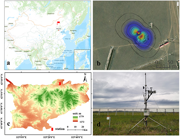
Figure 1. The eddy flux tower is at the position shown in the figure above (a). (b) shows the percentage contribution of fluxes (footprint) overlaid on a satellite image shown as RGB bands. (c) is the digital elevation map. (d) is the eddy covariance measurement instrument.
Download figure:
Standard image High-resolution image2.2. Micrometeorological measurements
The micrometeorological station consisted of above-ground and below-ground sensors and a datalogger (CR3000, Campbell, USA). The above-ground sensors were installed on the flux tower at a height of 2 m from the ground, and the probes of the below-ground soil monitoring system were at depths of 10 cm and 30 cm, respectively. The above-ground sensors mainly included air temperature and humidity, solar radiation, photometry, and wind speed and direction. The below-ground sensors were mainly composed of the soil monitoring system. The primary variables and sensor models are shown in table S1.
2.3. Eddy covariance measurements
The Open Path Eddy Covariance flux monitoring system consisted mainly of a three-dimensional ultrasonic anemometer (GILL WindMaster pro, GILL, UK) and an open path gas analyzer (LI-7500A, LI-COR, USA) for flux observations. The system comprised a miniature weather station and a high-frequency datalogger (Li-7550). The three-dimensional ultrasonic anemometer and infrared gas analyzer were mounted on top of the flux tower, which was 2 m high, with the main body made of galvanized steel pipes welded together, and the sensors were located above the vegetation canopy at a horizontal distance of 20 cm. The data collector was installed in an integrated box in the middle of the flux tower on the back side (placed in direct sunlight). A 12 V, 1200 Ah lead-acid battery was used for power supply, while a 60 W solar panel was used to charge the battery.
Differences in the main influences on atmosphere-surface carbon exchange can occur under different atmospheric stability conditions in the near-surface layer, as CO2 fixation and emissions vary with atmospheric stability. Monin–Obukhov theory is widely used as the main method for characterizing turbulent exchange within the atmospheric boundary layer (Foken 2006). The Monin–Obukhov atmospheric stability parameter ζ reflects the thermodynamic laminar stability of the atmosphere (Zoumakis and Kelessis 1993) and is calculated as follows:
where z is the height above the ground, d is the zero-displacement height, and l is the Monin–Obukhov length. The atmospheric stability condition data were divided into daytime and nighttime. Sixty-six percent of the daytime data were unstable conditions, 19% were neutral conditions and 15% were stable conditions. The nighttime data had 4% unstable conditions, 11% neutral conditions, and 85% stable conditions.
2.4. Calculation of daytime and nighttime NECB
To investigate the reliance of the NECB (μmol m−2 s−1) on multiple ecological factors, we separated the data within half-hour intervals into two distinct periods: the nongrowing season (NS) and the growing season (GS). We classified values in the PPFD (photosynthetic photon flux density) range of 50–2500 μmol m−2 s−1 as daytime data. During the growing season, we used the rectangular hyperbolic model proposed by Michaelis‒Menten to examine the relationship between PPFD and NECB (Michaelis and Menten 1913). This model effectively distinguishes the effects of daytime radiation and nighttime temperature on NECB. Rey et al (2012) used this model to analyze the carbon drivers of grassland ecosystems in semi-arid regions. Combined with the environmental similarity of alternating wet and dry seasons in the grasslands of Northern China, the study objectives were similar, so we also used this model in the study of the regulatory role of wind speed on NECB (figure 2):


Figure 2. The gray cube represents ecosystems. Relationship between carbon flux (C) from net ecosystem carbon balance (NECB) and carbon flux (bold) from net ecosystem production (NEP). The fluxes of NECB consist mainly of emissions to or uptake from the atmosphere of carbon dioxide (net ecosystem exchange, or NEE), carbon monoxide (CO), and volatile organic C (VOC); lateral or leaching fluxes of dissolved organic and inorganic C (DOC and DIC); lateral or vertical movement of particulate C (PC) (non-gaseous, non-soluble); fluxes that cause NEP are gross primary production (GPP), autotrophic respiration (AR), and heterotrophic respiration (HR). The blue box represents the influence process of wind speed.
Download figure:
Standard image High-resolution image
 is the ecosystem production rate at light saturation (μmol m−2 s−1), PPFD is the photosynthetic effective light quantum flux density incident on the leaf (μmol m−2 s−1), RE is ecosystem respiration, and k is the Michealis–Menten constant, whose value is the PPFD at which the photosynthetic rate reaches half of its maximum (
 ). It should be noted that CO2 absorption is coupled with a negative sign of NECB; therefore, GPP is negative in this situation.
We explored the connection between soil temperature and NECB during the nongrowing season and growing season, excluding rainfall events, utilizing night-time data (PPFD < 50 μmol m−2 s−1):

where  represents the CO2 exchange level at 0 °C, Tsoil represents the soil temperature at 10 cm below the surface (°C) and b is the fitting parameter associated with the Q10 value (a rise in NECB with a rise in temperature of 10 °C) in accordance with the equation:


where b is the fitting constant in the soil respiration and temperature index model, Re is the soil respiration rate, a is the fitting constant, and Tsoil is the soil temperature.
2.5. Partial correlation and structural equation modeling analysis of the driving factors of NECB
To analyze the bias correlation of the NECB response under the influence of wind speed with a particular meteorological factor, we controlled for the involvement or absence of wind speed to obtain the influence of other factors by wind speed. SPSS 25.0 for Windows was used for all statistical analyses (SPSS Inc., Chicago, Illinois, USA).
Structural equation modeling (SEM) analysis evaluated the standardized direct and indirect effects of the driving factors on NECB. We first tested whether all influential factors were collinearity (Jonsson et al 2010, Shi et al 2018). Then, we established two independent models in total, one part of wind speed affecting NECB through soil temperature (TS) and vapor pressure deficit (VPD) as the meteorological process model, and another model, the part affecting NECB through GPP and RE as the biological process model. After parameterizing the initial SEM with standardized data, we verified its goodness-of-fit by calculating the root mean square residual (SRMR), root mean square error of approximation (RMSEA), and goodness-of-fit index (GFI). Finally, we used the fit indices (0 < SRMR < 0.08, 0 ⩽ RMSEA ⩽ 0.05, and 0 < GFI ⩽ 1) to determine the most appropriate model for this study (Shi et al 2018). Analyses based on SEM were carried out in R (version 3.6.3; R Core Team, Vienna, Austria).
2.6. Constraint line definition and extraction
Multiple variables interact to influence ecosystem patterns and processes, which is why scatter plots illustrating the relationship between two ecological factors are commonly depicted as scatter clouds with boundaries, which do not indicate a correlation but represent a constraint. (Guo et al 1998, Hao et al 2022). Dependent variables cannot be completely controlled by independent variables; they can only be limited within a certain range by independent variables (Thomson et al 1996). Under the influence of the dependent variable, the constraint line indicates the extent of distribution or possible maximum or minimum value of the independent factor (Kaiser et al 1994). It has been suggested, however, that this approach should be coupled with other statistical techniques to better comprehend the ecosystem's nonlinear characteristics as well as to estimate the point at which the ecosystem will undergo significant changes (Qiao et al 2019).
To extract the constraint lines, segmented quantile regression was used (Jiang et al 2022). In figure S1, the horizontal and vertical coordinates represent wind speed and NECB, respectively. Firstly, the wind speed represented by the x variable is divided into 100 equal parts according to the numerical magnitude, so as to obtain 100 columns of the data set. Finally, the 100 upper boundary points and lower boundary points were fitted with the R program (https://cran.r-project.org/; R Core Team 2015) to obtain the constraint lines.
2.7. Preprocessing of data
Flux observation data from January 2017–December 2021 were selected for processing in this study. This study used the open-source EddyPro7.0.6 software (download at www.licor.com/env/support/EddyPro/software.html) for preliminary processing and calculation of 100 ms flux data after threshold screening (CO2 concentration of 100–1000 mg m−3 and water vapor concentration of 0–50 g m3), coordinate rotation correction (plane fitting method), frequency response correction, ultrasonic virtual temperature correction, and WPL correction (Aubinet et al 1999, Aubinet et al 2012, Wilczak et al 2001), the 30 min CO2 flux data (Webb et al 1980) were output, and further quality control was performed according to the following methods: (1) exclude the data of precipitation periods; (2) exclude the data of night data during periods of bad turbulence. Frictional velocity μ* is an essential parameter for turbulence characteristics, and too small of a μ* leads to too weak turbulent mixing and loss of confidence in the measured fluxes, so a nighttime u threshold (0.1 m s−1) must be set to filter out CO2 fluxes below this value; (3) the absolute median deviation method is used to remove outliers caused by equipment and the external environment (Falge et al 2001, Papale et al 2006); (4) evaluate the turbulence quality results of the software output using the '0-1-2' grading scale proposed by Lee et al (2004), where '0', '1', and '2' represent 'good', 'average', and 'poor' data quality, respectively. The convention specifies that photosynthesis by plants results in a negative flux of CO2 to the vegetation surface and positive respiration or from the surface to the atmosphere.
3. Results
3.1. Seasonal and interannual variability in micrometeorological conditions
There was little interannual variation in environmental factors. The multi-year averages of air temperature (Ta), soil water content (SWC), and net radiation (Rn) are 3.89 °C, 4.05% and 68.24 W m−2, respectively. Only the VPD showed a significant difference among the 5 years, which was 698, 651, 698, 619, and 593 Pa, respectively (figure 3). There were similar annual mean temperatures (about 3.88 ± 0.3 °C) and similar net radiation (ca. 68 ± 6 W m−2). From 2018 to 2021, the SWC (at 10 cm) was −5%, −7%, −9%, and 7% higher than that in 2017, respectively.
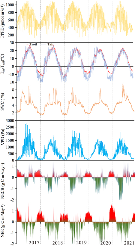
Figure 3. Changes in mean air temperature (°C), mean soil temperature (°C), mean soil volumetric water content (%), vapor pressure deficit (Pa), maximum direct photosynthetic photon flux density (μmol m−2 s−1), net ecosystem exchange (g C m−2 d−1) and net ecosystem carbon balance (g C m−2 d−1).
Download figure:
Standard image High-resolution imageHowever, a significant seasonal variation was observed in environmental factors. The minimum values of net radiation (Rn), air temperature (Ta), soil temperature (Ts) and VPD were in winter (−9.04 W m−2, −13.10 °C, −8.19 °C and 118.96 Pa, respectively) and the maximum values were in summer (135.59 W m−2, 18.84 °C, 20.49 °C and 1132.92 Pa, respectively). Despite slight differences in the seasonal averages, seasonal patterns of rainfall differed significantly within the study years (figure 3, table 1).
Table 1. The daily average Tair, Tsoil, wind speed (WS), soil water content (SWC), net ecosystem exchange (NEE), and net ecosystem carbon balance (NECB) for the growing season (GS) and nongrowing season (NS) were studied for five years. No. days represents the number of days in each period (2017/2021).
| Year | Period | No. days |
 (°C) (°C) |
 (°C) (°C) | SWC (%) | WS (m s−1) | VPD (Pa) | NEE (g m−2) | NECB (g m−2) |
|---|---|---|---|---|---|---|---|---|---|
| 2017 | NS | 153 | −9.72 | −4.52 | 3.10 | 3.57 | 175.10 | 94.88 | 82.68 |
| GS | 212 | 13.72 | 15.56 | 4.93 | 3.50 | 1056.70 | −60.58 | 19.26 | |
| Total | 365 | 3.89 | 7.14 | 4.16 | 3.53 | 687.15 | 4.59 | 45.84 | |
| 2018 | NS | 132 | −12.12 | −8.18 | 2.19 | 3.88 | 161.80 | 55.64 | 19.53 |
| GS | 234 | 11.85 | 13.35 | 4.84 | 3.76 | 890.21 | −151.98 | −68.04 | |
| Total | 365 | 4.46 | 5.60 | 3.89 | 3.81 | 629.22 | −38.92 | −36.56 | |
| 2019 | NS | 117 | −10.83 | −7.53 | 2.11 | 3.51 | 151.97 | 61.22 | 29.48 |
| GS | 248 | 11.40 | 12.63 | 4.72 | 3.53 | 965.66 | −144.95 | −99.67 | |
| Total | 365 | 4.27 | 6.17 | 3.88 | 3.52 | 704.83 | −78.86 | −58.27 | |
| 2020 | NS | 117 | −11.14 | −5.64 | 2.39 | 3.33 | 153.71 | 75.30 | 44.07 |
| GS | 249 | 10.76 | 12.34 | 4.49 | 3.56 | 848.65 | −158.98 | −111.85 | |
| Total | 366 | 3.76 | 6.59 | 3.81 | 3.49 | 626.50 | −84.07 | −62.01 | |
| 2021 | NS | 129 | −10.53 | −5.45 | 2.67 | 3.69 | 160.90 | 83.58 | 40.86 |
| GS | 236 | 10.87 | 12.55 | 5.33 | 3.49 | 804.12 | −162.17 | −70.85 | |
| Total | 365 | 3.31 | 6.19 | 4.39 | 3.56 | 576.79 | −75.31 | −31.37 |
3.2. Seasonal-scale variation in NECB
The NECB experienced a substantial seasonal change, with variations that were similar each year. The nongrowing season included parts of March and October, all of January, February, November, and December. (153, 132, 117, 117, and 129 d in the first, second, third, fourth, and fifth years, respectively). For most of the nongrowing season, the grassland ecosystem was a net source of CO2 (up to 3.47 μmol m−2 s−1 or 0.86 g C m−2 d−1) (figure 3). The total average sum of Compared to the average sum of NECB, NEE for the growing and nongrowing seasons each year was underestimated by 41.25, 2.36, 20.59, 22.06 and 43.94 g m−2, respectively.
During 2017, more carbon was lost during the nongrowing season than that was fixed during the remainder of the year. Therefore, the ecosystem acted as a carbon source. However, the remaining four years were the opposite, showing strong carbon sinks (table 1). There were 101.95, −48.21, −52.57, −67.78, and −30.00 g m−2 yr−1 of carbon released into the atmosphere from 2017 to 2021, respectively (figure 4). There was some carbon absorption by the ecosystem during the growing season (spring and summer), and the negative fluxes (maximum rates in spring 2021 of up to −2.43 g C m−2 d−1) always exceeded the positive fluxes during nongrowing seasons. In the spring, vegetation appeared to be most active (from April through June). This period was characterized by a large degree of variation within days of the same period, and the intensity of the change in the daily mean varies from year to year (figure S2).
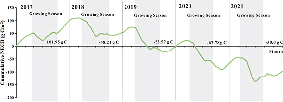
Figure 4. During the entire study period (2017–2021), the total amount of carbon exchanged (NECB) was calculated (g C m−2). The gray area represents the growing season.
Download figure:
Standard image High-resolution image3.3. Relationship between wind speed and NECB under different atmospheric stability conditions
The partial correlationship between wind speed and NECB at all times of the growing season was −0.14. When the partial correlation coefficients of TS, RN, VPD, and NECB were added to the wind speed, they changed by 11.54%, 1.39%, and 2.94%, respectively. The results showed that wind speed may play a moderating role in the relationship between TS and NECB, VPD, and NECB (table S2).
The relationship between wind speed and NECB varies significantly under different atmospheric stability conditions, but wind speed may have a more dramatic effect on the changes in carbon budget under unstable atmospheric conditions (figure 5). In the stable atmospheric condition, the amount of NECB remained essentially constant with increasing wind speed. However, under neutral as well as unstable atmospheric conditions, the variation of the lower constraint line of NECB had a similarity—decreasing first and then slowly increasing. We also found that the tipping point in both cases was in the range of 2–3 m s−1, indicating that the wind speed reached a maximum in this range for carbon fixation. Regarding the difference in the upper limit line between the two, the NECB was basically constant in the neutral condition, but the NECB amount increased and then decreased in the unstable case, implying that the carbon emission was increasing and then decreasing, while the wind speed reached its maximum in the range of 2–3 m s−1.

Figure 5. Relationship between wind speed (WS) (m s−1) and net ecosystem carbon balance (NECB) (μmol m−2 s−1) for the growing season (2017–2021) for different atmospheric stability conditions. The gray dots represent the data measured by the experiment. The red points represent the trend of carbon fixation by the ecosystem, and the green points represent the trend of carbon emission by the ecosystem. The red and green lines are fitted curves. The dashed yellow lines represent the balance condition of carbon absorption and discharge.
Download figure:
Standard image High-resolution image3.4. SEM analysis of the driving factors of NECB
Wind speed from the growing season mainly regulated NECB by affecting TS and VPD. Throughout the growing season, the meteorological factor part of the model explained 48% of the variance in NECB, 15% of the variance in VPD, and 15% of the variance in TS, with an indirect negative effect of wind speed on NECB (−0.38, through VPD and TS) and a negative direct effect (−0.18). The biological process part of the model explained 68% of the variance in NECB, 4% of the variance in RE, and 3% of the variance in GPP, with an indirect negative effect of wind speed on NECB (−0.19, through GPP and RE) and a negative direct effect (−0.15) (figure 6(a)). In the case of stable atmospheric stability, there was an indirect negative effect of wind speed on NECB (−0.12, through VPD and TS) and a negative direct effect (−0.15) in the meteorological factor model part; in the effect on the biological process part, there was an indirect negative effect of wind speed on NECB (−0.04, through GPP and RE) and a negative direct effect (−0.13) (figure 6(b)). In the case of neutral atmospheric stability, there was an indirect negative effect of wind speed on NECB (−0.16, through VPD and TS) and a negative direct effect (−0.17) in the meteorological factor model part; in the effect on the biological process part, there was an indirect negative effect of wind speed on NECB (−0.18, through GPP and RE) and a negative direct effect (−0.19) (figure 6(c)).

Figure 6. Structural equation model (SEM) of the effect of wind speed on net ecosystem carbon balance (NECB) in semiarid grassland. In the graph, the path strengths have been displayed using the standardized correlation coefficients. The blue arrows indicate positive correlations, and the red arrows indicate negative correlations. The R2 values at the corners of the rectangles indicate the percentage of variance that can be explained by other variables in relation to these points. Numbers represent the total effect of driving factors on NECB. a represents all time periods of the growing season, and b, c, and d represent the stable, neutral, and unstable atmospheric stability scenarios of the growing season, respectively.
Download figure:
Standard image High-resolution imageWe found that wind speed significantly affected the overall ecosystem under unstable atmospheric stability during the growing season. There was an indirect negative effect of wind speed on NECB (−0.26, through VPD and TS) and a negative direct effect (−0.16) in the meteorological factor model part; in effect on the biological process part, there was an indirect negative effect of wind speed on NECB (−0.06, through GPP and RE) and a negative direct effect (−0.18) (figure 6(d)).
3.5. Relationship between wind speed and heat transfer
The relationship between wind speed, NECB, and sensible and latent heat flux was analyzed to characterize the effect of wind speed on the surface energy balance under different atmospheric stability conditions (figure 7). When atmospheric stability was unstable (−1 ⩽ ξ ⩽ −0.01), carbon uptake was at its maximum, and sensible and latent heat fluxes were also at their maximum, indicating the most rapid energy transfer. At ξ = −0.55, the carbon fixation of the ecosystem reached its maximum value, and the sensible and latent heat fluxes were the largest at this time, but as the wind speed increased, the sensible and latent heat fluxes decreased rapidly, and carbon emissions increased rapidly. When the atmospheric stability was neutral (−0.01 ⩽ ξ ⩽ 0.01), the wind speed decreased rapidly, the NECB increased, the carbon emission increased, and the sensible and latent heat fluxes decreased rapidly; when the atmospheric stability was stable (ξ > 0.01), the nighttime data accounted for 85%, and the carbon balance, sensible and latent heat fluxes and wind speed were more stable and remain unchanged.

Figure 7. During the growing season, the relationship between WS (wind speed, m s−1), H (sensible heat flux, W m−2), LE (latent heat flux, W m−2) and NECB (μmol m−2 s−1) for different atmospheric stability conditions is shown by blue, red and green dots, respectively. Each data point is binned according to the Monin–Obukhov atmospheric stability parameter  (each 0.002).
Download figure:
Standard image High-resolution image
4. Discussion
4.1. Seasonal and diurnal variation of NECB
During the five years, vegetation fixed a large amount of CO2 during the growing season, and vegetation was dormant during the non-growing season and no longer fixed CO2, which created a carbon balance curve with a trough in spring and summer, and a peak in autumn and winter. The climate was one of the main factors influencing ecosystem carbon fluxes, and the carbon source presented throughout 2017 was precisely due to drought that inhibited grass growth during the growing season, indicating that the carbon balance in Northern China was mainly dominated by changes in precipitation (Wang et al 2020). It has been shown that in drought years, ecosystems were converted from carbon sinks to carbon sources (Zhang et al 2020). In contrast, the degree of plant activity during the non-growing season was determined by temperature (Fu et al 2019).
Daily CO2 fluxes varied significantly among seasons and slightly among years. The negative daily CO2 fluxes were mainly in the growing season from April to October, and it was noteworthy that the positive fluxes dropped to near zero in the morning of the growing season, around 6:00–8:00, probably as a result of photosynthetic activity, and the carbon fixation rate reached its maximum around 12:00, but the carbon sink capacity decreased with increasing radiation, probably related to the closure of stomata (Wehr et al 2021). However, in the morning of the non-growing season, the vegetation was inactive and there was still a small amount of carbon fixation, probably due to the effective moisture of the morning dew that promoted the growth of the biological crust (Grote et al 2010).
4.2. The moderating effect of wind speed on ecosystem carbon balance
Wind speed had a strong moderating effect on meteorological factors such as surface temperature and precipitation. For the variation of moisture, the higher the wind speed, the higher the evaporation (Swelam et al 2010). We used unstable atmospheric conditions data, which represents the daytime data of vegetation productivity accumulation, and found that wind speed influences carbon balance contribution up to 0.41 through TS and VPD by SEM, which also indicated that wind speed had a strong driving force on material movement and energy exchange, such as soil moisture and temperature. Some studies had shown that micrometeorology was determined by the evolution of the atmosphere and surface boundary layer soils at small scales, which included the absorption and release of radiant energy by plants and soils, and the interaction of wind with plants and the surface boundary layer causing the transfer or flow of materials and energy (Lee 1998, Munn et al 2013). Changes in wind speed and the interaction between vegetation and soil led to changes in surface temperature and moisture content. For example, areas with significantly stronger winds were drier and had lower soil moisture content in early spring, mid to late summer, and early fall; higher wind speeds were more likely to become rain-free in the latter part of summer than in areas with weaker winds (Mezösi et al 1998, Fu et al 2022). There existed a corpus of studies whose findings align with our results. The impact of wind on atmospheric temperature and humidity is well-established, as changes in wind speed can significantly modulate the fluxes of heat and water vapor between the ground and the atmospheric boundary layer. This modulation encompasses alterations in the temperature of the lower atmosphere and the near-surface VPD, ultimately exerting consequential effects on the growth of vegetation (Colazo et al 2015, Yuan et al 2019).
We found that wind speed affected the rate of surface heat transfer in different atmospheric stability conditions. When atmospheric stability was stable (0.01 ⩽ ξ ⩽ 1), changes in heat as well as carbon balance were insignificant, indicating that environmental variables and vegetation conditions were relatively stable, and it was found statistically that 85% of the data in this case occur at night; When in the unstable case (−1 ⩽  ⩽ −0.01), if the wind speed exceeded 2.35 m s−1, both sensible and latent heat fluxes decreased sharply and carbon emissions increased. The main reason was that turbulent winds can change the mixing between atmospheric boundary layer conditions, wind speed and turbulence, directly affecting the vertical energy distribution and energy exchange between the atmosphere and the surface boundary layer-when wind speed exceeded a threshold, energy exchange accelerated and the surface-atmosphere heat difference decreases, thus affecting the surface microclimate and further leading to increased carbon emissions (Armstrong et al
2014). Of course, the increase in carbon emissions may also be related to CO2 expulsion from soil pores. Soil CO2 production decreases with depth and occurs primarily at the surface (Rey et al
2008). An air-filled network of pores connected the surface of the soil to the deeper layers of soil, which facilitated the movement of CO2. In contrast to CO2 movement through the soil profile, which was primarily guided by diffusion, the flow of CO2 through porous, fractured, and dry subsoils, as well as release at the surface-atmosphere interface, was largely determined by differential pressure gradients, wind gusts, and turbulence (Jassal et al
2004, Sun et al
2007, Rey et al
2012). Experimental observations of the effects of decreasing wind speed on carbon fluxes in grassland ecosystems using wind-blocking facilities in a typical grassland in Inner Mongolia showed that the ecosystem respiration rate, soil respiration rate, and net ecosystem carbon exchange were lower in grassland ecosystems on the windward side with higher daytime wind speed than on the leeward side with lower wind speed (Jin 2014). In contrast, experimental observations in a semiarid grassland in southeastern Spain showed that wind speed changes could only affect CO2 variation from the soil during the day, while at night, the wind speed could not affect carbon change due to the pressure of mechanical turbulence on convective turbulence (Rey et al
2012).
⩽ −0.01), if the wind speed exceeded 2.35 m s−1, both sensible and latent heat fluxes decreased sharply and carbon emissions increased. The main reason was that turbulent winds can change the mixing between atmospheric boundary layer conditions, wind speed and turbulence, directly affecting the vertical energy distribution and energy exchange between the atmosphere and the surface boundary layer-when wind speed exceeded a threshold, energy exchange accelerated and the surface-atmosphere heat difference decreases, thus affecting the surface microclimate and further leading to increased carbon emissions (Armstrong et al
2014). Of course, the increase in carbon emissions may also be related to CO2 expulsion from soil pores. Soil CO2 production decreases with depth and occurs primarily at the surface (Rey et al
2008). An air-filled network of pores connected the surface of the soil to the deeper layers of soil, which facilitated the movement of CO2. In contrast to CO2 movement through the soil profile, which was primarily guided by diffusion, the flow of CO2 through porous, fractured, and dry subsoils, as well as release at the surface-atmosphere interface, was largely determined by differential pressure gradients, wind gusts, and turbulence (Jassal et al
2004, Sun et al
2007, Rey et al
2012). Experimental observations of the effects of decreasing wind speed on carbon fluxes in grassland ecosystems using wind-blocking facilities in a typical grassland in Inner Mongolia showed that the ecosystem respiration rate, soil respiration rate, and net ecosystem carbon exchange were lower in grassland ecosystems on the windward side with higher daytime wind speed than on the leeward side with lower wind speed (Jin 2014). In contrast, experimental observations in a semiarid grassland in southeastern Spain showed that wind speed changes could only affect CO2 variation from the soil during the day, while at night, the wind speed could not affect carbon change due to the pressure of mechanical turbulence on convective turbulence (Rey et al
2012).
4.3. Suitable wind speed promotes the growth of vegetation
The wind is one of the leading environmental variables that significantly affect plant growth, development, and distribution, and extensive research has been conducted on the effects of wind on plants (Dixon et al 1984, De et al 2008). The effects of wind on plant growth are complex, both direct and indirect, with the wind being able to alter plant morphology and affect plant growth through direct contact, as well as indirectly affecting plant physiological traits by altering the transfer and transport of heat, water vapor, and carbon dioxide to influence gas exchange (Grace 1988, Ennos 1997, James, 2006). The effect of wind speed on plants is twofold: an appropriate wind speed can increase the exchange of materials and energy between plants and soil and the atmosphere and accelerate plant growth, but an excessive wind speed, which exceeds the capacity of plants, can cause damage to plants and inhibit plant growth (Van et al 1991, Cleugh et al 1998, Li et al 2009). Even only brief exposure to wind can lead to significant plant size, leaf area, and crop yield reductions (Grace 1988). The wind effect changes the plant growth rate and leaf morphology, resulting in radial expansion of stems, increased leaf thickness, reduced stem elongation, and reduced leaf area, and affects cell synthesis; wind-induced plant movements such as friction between plant leaves can cause abrasion of the superficial waxy layer on the leaves, resulting in increased epidermal conductivity and water loss; when wind speed exceeds the plant's capacity, plant leaves can be torn, peeled and worn when the wind speed exceeds the plant's capacity, and even the vegetation will fall over directly, while the soil particles blown by the wind may also wear and damage the plant tissues (Pitcairn et al 1986, Vogel 2009, Onoda and Anten 2011). The mechanical effects of wind on plants also affect the internal structure of plants, which in turn affects their water regulation and photosynthetic physiology (Clark et al 2000). The wind speed dictates the conductivity of the leaf boundary layer, which directly affects the rate of photosynthesis, transpiration, and leaf temperature according to the energy balance equation (Daudet et al 1999). The plant transpiration rate varies with wind intensity, duration, and species, and wind speed can increase the plant transpiration rate. However, wind speeds above a certain threshold will decrease the transpiration rate (Woolley 1961, Huang et al 2015). In summary, through this study we also suggest the establishment of low-wind zones, such as windbreaks, to protect the growth of vegetation in semi-arid areas with extremely fragile ecological environments.
5. Conclusion
In summary, in this study, we concluded that a wind speed reduction attenuates the adverse effects of climate change (changes in precipitation and temperature) on vegetation carbon balance. The effect of wind on vegetation is not linear, but there is a threshold value. Vegetation growth is most favorable when wind speed is in the range of 2–3 m s−1. When using only NEE to measure the carbon balance of an ecosystem, we vastly underestimate the carbon emission capacity because we do not consider the inorganic carbon in the ecosystem. The effect of wind speed on the carbon balance of boreal grassland ecosystems is mainly influenced by the regulation of micrometeorology. Therefore, in the study of meteorological factors influent carbon balance, we should not neglect the impact of strong and gentle winds on vegetation, which may be as important as the impact of precipitation and temperature on vegetation in the region. We suggest that the establishment of low wind zones as part of soil conservation efforts may have had some positive impact on the carbon balance of grasslands in semi-arid regions.
Acknowledgments
We appreciate the editors' and anonymous reviewers' suggestions for improving our manuscript. We sincerely thank the personnel who worked on the experimental field observation in Taipusi Banner, Inner Mongolia Autonomous Region. We would like to thank the high-performance computing support from the Center for Geodata and Analysis, Faculty of Geographical Science, Beijing Normal University. This research was funded by the National Key Research & Development Program of China (Grant Number 2017YFA0604902), Project Supported by State Key Laboratory of Earth Surface Processes and Resource Ecology, Guangxi University High-level Talent Program (A3100051013).
Data availability statement
The data cannot be made publicly available upon publication because they are not available in a format that is sufficiently accessible or reusable by other researchers. The data that support the findings of this study are available upon reasonable request from the authors.
Supplementary data (0.2 MB DOCX)