

Abstract
Summer heatwaves repeatedly affect extended regions in Europe, resulting in adverse economic, social, and ecological impacts. Recent events, e.g. the 2022 heatwave, also attract interest regarding the spatial shifts of their impact centers. Evaluations so far either investigated heatwave passages at pre-defined locations or employed algorithms to spatio-temporally track their core regions. Usually, the latter focus on single events, and thus often fail to generalize spatial heatwave tracks or ignore track characteristics. Here, we use a data-driven approach employing causal discovery to robustly characterize European heatwave tracks in single-model initial condition large ensemble (SMILE) climate simulations to overcome sampling uncertainties of observational records. This enables us to identify specific recurrent heatwave tracks, evaluate their preferential seasonal occurrence, and associate them with moving high pressure centers. Additionally, the evaluation of heatwave track representation in the SMILE extends standard model evaluation, which is mostly based on static statistics. We provide the first comprehensive analysis on heatwave tracks considering internal climate variability conducted within a SMILE, promoting the latter as a methodological testbed in climate extremes research.
Export citation and abstract BibTeX RIS

Original content from this work may be used under the terms of the Creative Commons Attribution 4.0 license. Any further distribution of this work must maintain attribution to the author(s) and the title of the work, journal citation and DOI.
1. Introduction
Due to their frequent and often persisting occurrences in extended European regions, heatwaves accounted for substantial economic, social, health, and ecologic impacts and loss during the past years.
Local heatwave occurrence is commonly associated with various dynamic or thermodynamic drivers. Dynamic drivers include anticyclonic, sometimes quasi-stationary ('blocking') conditions fostering local heating during subsidence processes or heat advection (Lhotka et al 2018, Simmonds 2018, Shafiei Shiva et al 2019, Li et al 2020, Suarez-Gutierrez et al 2020). Blocking is known to be connected to Northern Hemisphere temperature extremes (see also Zhuo et al 2022). Thermodynamic drivers refer to soil moisture conditions affecting evaporative cooling (Hirschi et al 2011, Jaeger and Seneviratne 2011) or local and upwind land-atmosphere coupling (Fischer et al 2007, Lhotka and Kyselý 2015b, Schumacher et al 2019) which may both be influenced by preceding seasonal precipitation deficits (Della-Marta et al 2007, Vautard et al 2007, Bastos et al 2020, Felsche et al 2022). Associated to the latter, anthropogenic land use changes like albedo effects, humidity and radiation budget changes due to imperviousness alteration, i.e. urbanization, regionally explain considerable portions of heatwave variability (Li et al 2021, Wu et al 2021). Studies show that favorable projected changes in these drivers or their combinations imply increases in heatwave number, duration, and intensity under changing climate conditions which stresses the importance of quantifying heatwave characteristics (Meehl and Tebaldi 2004, Shafiei Shiva et al 2019, Molina et al 2020, Suarez-Gutierrez et al 2020) for adaptation.
Additionally, scientific knowledge on geographical heatwave characteristics is key to adaptation, be it the derivation of distinct geographical heatwave regions in Europe by means of clustering (Stefanon et al 2012), the integration of spatio-temporal characteristics in a heat severity index (Keellings and Moradkhani 2020), inter-model differences of typical spatial patterns (Gibson et al 2017, Molina et al 2020), or ranking of historical events regarding their extent and intensity (Russo et al 2015, Lhotka and Kyselý 2015a, 2015b). Depending on the size and shape of regions affected by heatwaves, people exposure and energy demand for cooling may increase, especially in regions not acclimatized to high temperatures (Smith et al 2013, Lyon et al 2019). While the spatial extent of heatwaves is captured by temporally aggregated measures like the heatwave magnitude index daily (HWMId, Russo et al 2015), they miss the temporal evolution of heatwaves.
Increased knowledge on the spatio-temporal evolution of heatwaves offers the opportunity for warning and preparation along their propagation pathways (Clemesha et al 2018, Lo et al 2021). Thus, not only defining static heatwave regions, but also considering their time-dependent positions is crucial in heatwave prediction (Clemesha et al 2018), analysis (Sánchez-Benítez et al 2020, Lo et al 2021), or impact assessment. For example, Stefanon et al (2012) present the temporal sequence of spatial European heatwave clusters, but without further investigating potentially preferential sequences. Clemesha et al (2018) investigate the propagation and characteristics of observed California heatwaves when passing pairs of distinct geographical regions. Others follow a Lagrangian perspective by determining major heating processes within European heatwave trajectories (Bieli et al 2015, Zschenderlein et al 2019), or by tracking global drought displacement (Herrera-Estrada et al 2017, Herrera-Estrada and Diffenbaugh 2020). Spensberger et al (2020) find that one observed transition among heatwaves in distant regions, Central European–Scandinavian successions in 2003 and 2018, occurred coincidentally based on dynamics investigations.
These analyses do not generalize heatwave track characteristics and fail to explain the reasons of specific tracks. Thus an approach to (a) derive typical heatwave tracks, and (b) summarize track specifics is needed, in order to (c) associate tracks with explanatory variables. We attempt to extend and generalize the idea of establishing dynamical links among heatwaves occurring in close temporal and spatial vicinity.
An elegant solution to derive directed links among spatio-temporal phenomena, including the information on link significance, effect size, and temporal lags of signal propagation, is provided by causal discovery algorithms. Causal discovery or causal inference allows harvesting the potential of climate big data to gain knowledge on processes by deriving hypotheses on causal interdependence hidden in (observational) data (Ebert-Uphoff and Deng 2012a, Deng and Ebert-Uphoff 2014, Runge et al 2019a, 2019b). More specifically, Runge et al (2019b) mention causal hypothesis testing, climate network analysis, driver identification with respect to extreme impacts or model evaluation as potential applications in climate research. So far, causal discovery was used to obtain networks of information flow within the atmosphere, e.g. portraying westerly atmospheric flows (Ebert-Uphoff and Deng 2012b), or the identification of major atmospheric perturbation 'gateways' related to teleconnections (Runge et al 2015). Almendra-Martín et al (2022) use a causal discovery algorithm to identify the influence of climate modes on soil moisture variability. Very recently, first climate model ensemble based investigations of teleconnections were performed (Galytska et al 2022, Karmouche et al 2022).
Transferring the concept of information flow (Runge et al 2015) to the heatwave propagation question, we suggest interpreting heatwave movements as temporally lagged heatwave onset in distinct regions. We propose a generalized approach to explain heatwave propagation based on causal discovery and examine potential explanations for derived pathways. This study builds on results from a previous study (Felsche et al 2022), where recurrent heatwave core regions were derived by means of clustering. We hypothesize that distinct recurring propagation tracks can be identified beyond single events in Europe. To generalize from observed event sequences we employ a single-model initial condition large ensemble (SMILE) of a regional climate model. This increases the sample of potential heatwave tracks and allows to evaluate observed tracks with respect to naturally occurring climate variability in high spatio-temporal resolution.
2. Methodology
Our approach to track heatwaves consists of four steps: (a) define each day within the analysis period meeting preset criteria as a heatwave (hot day), (b) cluster all hot days with respect to their geographical extent into core regions, (c) aggregate these core regions into time series and (d) apply a causal discovery algorithm to derive directed links among the core region time series.
2.1. Data and validation
Observational records provide a limited amount of heatwave events in Europe. Thus, employing a SMILE allows to increase the sample size: By using the Canadian Regional Climate Model, version 5, Large Ensemble (CRCM5-LE, Leduc et al 2019) we obtain 50 members of comparable climate statistics to derive robust results at high spatial resolution (0.11∘, 12.5 km) while considering internal climate variability. While the CRCM5-LE was already extensively used for analyses on rare (hydrometeorological) extremes (Champagne et al 2020, Wood and Ludwig 2020, Böhnisch et al 2021, Brunner et al 2021, Poschlod and Ludwig 2021), the present study is the first to apply causal inference where large samples are also of importance (Spirtes and Glymour 1991, Runge et al 2019b).
We pool the period 1981–2010 from 50 members into one 1500 year time series. Since all members are designed to share comparable climate statistics, typical patterns and subsequently pathways of phenomena are assumed to be comparable across all members (and to reality), only varying due to internal climate variability (Leduc et al 2019).
For heatwave definition, we use daily maximum temperature (tasmax). Daily 500 hPa geopotential height (Z500) is employed for large-scale atmospheric pattern definition. We first perform heatwave clustering and track derivation on a ERA-Interim driven (Dee et al 2011) run of CRCM5 (CRCM5/ERA, Leduc et al 2019) in order to evaluate them against historical events while using the same regional climate model. Additionally, an external evaluation on the E-OBS gridded dataset (version 22.0e at 0.1∘ spatial resolution; Haylock et al 2008, Cornes et al 2018) is performed (figure S1). All analyses are confined to land areas within a European domain (Leduc et al 2019).
2.2. Heatwave definition
Heatwave definitions in literature vary according to study perspectives (Perkins and Alexander 2013, Smith et al 2013, Shafiei Shiva et al 2019). To properly assess heatwave tracks, our heatwave definition requires information for each time step (day) under consideration. We define heatwaves relative to local climatology (Della-Marta et al 2007) as a minimum of three consecutive hot days, separated by at least three non-hot days (Keellings and Moradkhani 2020, Spensberger et al 2020) from the preceding/following hot day: a hot day occurs if the centered three-day-running mean of tasmax exceeds the local 95th JJA (1981–2010) percentile (similar to Lhotka and Kyselý 2015a). Negative anomalies are omitted. Whereas the percentile in a single run or observations/reanalysis may be poorly estimated due to the limited sample size (30 years), uncertainty due to internal variability is reduced in the SMILE by deriving the percentile from a 1500 year sample. Additionally, percentile based anomalies reduce potential inconsistencies among the data sources induced by climate model bias.
Spurious artifacts ( pixels) and isolated hot day occurrences are removed. A time step is considered as belonging to an extended heatwave event, if hot days occur in at least
  of the land area in the domain (i.e. 500 grid cells). All matching time steps are next used to derive core regions by clustering (Felsche et al
2022). Preliminary analyses revealed hot days in months May–October, such that we splice this period over all years and members (Ebert-Uphoff and Deng 2012a).
of the land area in the domain (i.e. 500 grid cells). All matching time steps are next used to derive core regions by clustering (Felsche et al
2022). Preliminary analyses revealed hot days in months May–October, such that we splice this period over all years and members (Ebert-Uphoff and Deng 2012a).
2.3. Location of core regions
For core region definition, we refer to spatially coherent recurring patterns of European heatwaves by means of clustering (Felsche et al 2022).
Clustering is frequently employed for mid-latitude weather pattern analysis and classification (Smyth et al 1997, Stefanon et al 2012, Lhotka and Kyselý 2015a, Hannachi et al 2017, Wang et al 2018, Keellings and Moradkhani 2020, Machado and Lopes 2020). We use daily maps of hot day occurrences as input to a two-step agglomerative hierarchical clustering (Felsche et al 2022). The optimal number of clusters is determined by computing the distortion score for every possible number of clusters and piking the knee of the curve (Jung et al 2003). When comparing cross-validation clustering results against cluster results from a Monte–Carlo pseudo-experiment, nine spatial heatwave patterns are obtained which are significant on the 99% level based on a two-sided t-test (Felsche et al 2022). These cluster footprints correspond well with historical events captured by other heatwave indexes (e.g. Russo et al 2015). Felsche et al (2022) shows high consistency among clusters in CRCM5/ERA and CRCM5-LE. We follow their naming conventions for CRCM5-LE: BI (Britain and Ireland), IP (Iberian Peninsula), WE (Western Europe), CEE (Central-Eastern Europe), SCA (Scandinavia), NEE (North-Eastern Europe), SEE (South-Eastern Europe), GSI (Greece/Southern Italy). Sequences of time steps labeled according to their respective clusters then represent single heatwaves (figure 1).
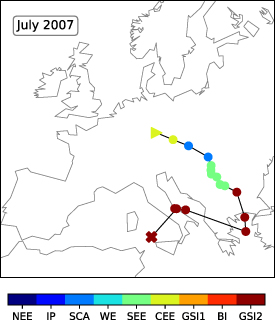
Figure 1. Conceptual heatwave representation: points show the daily centroids of heatwave footprints (Lo et al 2021) of the 2007 heatwave (CRCM5/ERA data), colored by the cluster labels which were assigned to the corresponding time steps. Triangle (cross) marks starting (ending) position of the heatwave. Cluster names: BI (Britain and Ireland), IP (Iberian Peninsula), WE (Western Europe), CEE (Central-Eastern Europe), SCA (Scandinavia), NEE (North-Eastern Europe), SEE (South-Eastern Europe), GSI (Greece/Southern Italy).
Download figure:
Standard image High-resolution imageNext, clustered time steps are spatially averaged, using the normalized intensity of temporally averaged cluster footprints as weights for their centroid coordinates (Herrera-Estrada et al 2017, Herrera-Estrada and Diffenbaugh 2020, Sánchez-Benítez et al 2020). This provides nine time series of positive temperature anomalies, located at the cluster footprint centers (i.e. their centroids) and representing the components (Runge et al 2015) among which spatio-temporal links are to be established. A sensitivity experiment using different weights for aggregation and therefore time series positioning revealed no major changes in link directions. Since CRCM5/ERA and CRCM5-LE provide slightly different cluster footprints, the positions of these time series diverge as well (see figure 2(a) and figure S1 for E-OBS).

Figure 2. (a) Centroid positions (blue dots) of core regions of CRCM5/ERA and CRCM5-LE superposed on the 1981–2010 JJA tasmax 95th percentile. S-score = 0.98 among percentiles of CRCM5/ERA and CRCM5-LE (Nowack et al
2020). Barplots indicate relative frequency of regional starting ( ) and ending (
 ) of heatwaves. (b) Cluster transitions in CRCM5/ERA data 1981–2010. (c) Frequency of transitions per heatwave against length of heatwaves (days) for CRCM5-LE (orange) and CRCM5/ERA (dark red).
Download figure:
Standard image High-resolution image2.4. Transitions among core regions by means of causal discovery
In order to analyze heatwave tracks between heatwave onset and offset, we split them into transitions among core regions. This captures direct movements between various regions. Location changes within cluster regions or growth and shrinkage of the spatial extent without heatwave core shifts are considered as stationary.
A heatwave moves from region A to region B, if heatwave onset in region A is followed by heatwave onset in region B, and if heatwave onset in region B was preceded by heatwave onset in region A: The heatwave stays in region A until day t and moves to region B at day t+1. We thus aim to explain a later position of a heatwave by its previous position (i.e. effect preceded by its cause).
Generally in causal discovery, distinct nodes representing single processes (variables or locations of the same variable) are derived prior to link establishing, by e.g. sampling of equally spaced grid points or rotated principal component analysis (Ebert-Uphoff and Deng 2012b, Deng and Ebert-Uphoff 2014, Runge et al 2015, 2019a, Nowack et al 2020). Here, we employ time series assigned to nine spatially distributed clusters of heatwave core regions.
To define linear spatio-temporal links among heatwave core regions we employ a causal discovery algorithm provided with the Tigramite 5.1 Python package, namely the PCMCI algorithm (Runge et al 2019a, Nowack et al 2020). It is based on the PC algorithm introduced by Spirtes and Glymour (1991): First, a fully connected graph of all variables (nodes) under consideration, e.g. time series at different locations, is created. Then, conditionally independent links (edges) are deleted, while for the remaining links directions are identified (e.g. by considering a temporal ordering of cause and effect) (Ebert-Uphoff and Deng 2012a, Deng and Ebert-Uphoff 2014, Runge et al 2019b). An amelioration with respect to time series is provided by the two-step PCMCI algorithm, adding a momentary conditional independence test to the PC algorithm (Runge et al 2019a, Nowack et al 2020): it rejects spurious or indirect links by testing for independence conditional on the common past of network nodes. Thus, only direct links among network nodes are kept which goes beyond pure pairwise correlation graphs (Runge et al 2019b). The PCMCI algorithm can be more powerful than correlation analysis in determining relationships between variables, even in finding links which may not be obvious in classic correlation analysis (Almendra-Martín et al 2022). Additionally, it bears the potential to find indirect links and consider common drivers as opposed to other forms of causal discovery like Granger causality (Granger 1969, Runge et al 2019b, Galytska et al 2022).
In this present study, conditional independence tests are conducted based on partial linear correlations (ParCorr) with a significance threshold of  . We use a minimum temporal lag of one day, reflecting transitions, and a maximum of three days, reflecting the three days separating two heatwaves. Additionally, we focus on positively correlated links because negative correlations would correspond to the non-occurrence of heatwaves in region B after occurrence in region A.
2.5. Explaining heatwave tracks
The importance of heatwave drivers varies regionally (Zschenderlein et al 2019), with dynamical mechanisms generally dominating over local thermodynamical ones (Suarez-Gutierrez et al 2020). As mentioned previously, high pressure, i.e. positive Z500 height anomalies, may lead to subsidence, cloud dispersal and subsequently enhanced heating at the surface. Additionally, prevailing dry conditions, e.g. low soil moisture contents, amplify the heating process by reducing the latent heat flux. Both drivers may interact and intensify, e.g. in feedback loops (Fischer et al 2007), since prevailing heat in turn may increase evaporation, thereby leading to further soil drying (Schumacher et al 2019).
We focus on associated large-scale Z500 conditions to investigate why heatwaves follow a given track. Patterns similar to the Z500 anomaly composites alongside selected heatwave transitions are searched during months May–October. Thereupon we calculate the probabilities of (a) having this pattern during an eight-day period centered at the indicated transition and (b) of having this transition during the indicated pattern. Pattern similarity is assessed by means of masking: if at least 66% of grid cells at an arbitrary time step show positive anomalies inside the composite positive anomaly region, and if at the same time an analogous agreement is achieved within the composite negative anomaly region, this time step is considered as being similar to the composite pattern. Consecutive days of similar patterns are summarized as one occurrence, which is related to atmospheric circulation persistence (see Jézéquel et al 2018, who relate atmospheric patterns to hot days by means of Euclidean distance calculation).
3. Results
3.1. Spatial propagation of heatwaves
During 1981–2010, 115 European heatwaves with at least three days are identified in CRCM5/ERA compared to 5425 in the 50-member CRCM5-LE. Most heatwaves occur during summer months JJA, starting earlier in the West than in the East (Felsche et al 2022). The relative frequency of heatwaves ending in the Eastern parts of Europe is increased compared to the frequency of heatwaves starting there (figure 2(a)). Accordingly, heatwaves start more frequently in the Western parts of Europe. Taken together, these first findings indicate a general west-to-east movement of heatwaves in both CRCM5/ERA and CRCM5-LE, which mirrors the dominating westerly flow onto Europe (e.g. Zschenderlein et al 2019). Heatwaves starting outside the defined core regions, e.g. outside the domain, over Northern Africa or the ocean, are not captured.
Most heatwaves consist of several transitions (figures 2(b) and (c)). While in general the number of transitions increases with heatwave length, very stationary heatwaves extend up to 20 days within one cluster and highly mobile heatwaves encounter 6 transitions in ten days. CRCM5-LE shows a stronger variability among transition–length combinations than CRCM5/ERA, representing natural variability of heatwave characteristics. The three historical examples 2003, 2006, and 2010 exhibit extreme lengths with respect to the majority of events (e.g. three transitions in 44 days in 2010).
A more detailed network of statistical robust sequences among neighboring core regions is provided in figures 3(a) and (b). It represents a mixture of latitudinal and longitudinal transition directions like a spine of the continental landmasses: While in the West, a South-Northward direction prevails, the East experiences the opposite direction. Within the scope of our study, we focus on links with lag  among two core regions at a time. In order to obtain robust results, links were first derived on the entire 1500-summer period. To include internal variability of these, they were also calculated for each member separately, allowing to count their frequency. In figure 3, only links occurring in at least 15 members (i.e. 30% of the ensemble) are presented with colors indicating their frequency (compare Galytska et al
2022, Karmouche et al
2022, for alternative presentation methods in ensembles). As a real-world example, the July 2007 heatwave (figure 1) is represented within the SEE–GSI link.
among two core regions at a time. In order to obtain robust results, links were first derived on the entire 1500-summer period. To include internal variability of these, they were also calculated for each member separately, allowing to count their frequency. In figure 3, only links occurring in at least 15 members (i.e. 30% of the ensemble) are presented with colors indicating their frequency (compare Galytska et al
2022, Karmouche et al
2022, for alternative presentation methods in ensembles). As a real-world example, the July 2007 heatwave (figure 1) is represented within the SEE–GSI link.

Figure 3. (a) Connections among core regions according to PCMCI algorithm in CRCM5-LE. Coloring indicates number of members with given link (required minimum of 15 links, i.e. 30%). (b) mean link occurrence per member in leave-one-out analysis of nodes.
Download figure:
Standard image High-resolution imageIn order to further evaluate the obtained links, we next compare the graph based on model data with reanalysis and observation based links (compare Karmouche et al 2022). While most of these links figure in the CRCM5/ERA and E-OBS network as well (figures S1(a) and (c)), several links from historical data are missing within the robust CRCM5-LE links, being thus (most likely) rare outliers. Others are shifted compared to CRMC5-LE since the position of core regions diverges. The CRCM5-LE links show higher correspondence to the representation in CRCM5/ERA (F1-scores among members and reference above 0.5, figure S2) than to the one in E-OBS (F1-scores close to 0.2; most likely due to clearly shifted or split core regions like, e.g. GSI). Additionally, no link connecting CEE and SCA can be established in CRCM5/ERA as was also found in Spensberger et al 2020. Since CRCM5-LE shows these links in 16 and 30 members, respectively, it is likely not observed in CRCM5/ERA due to potential errors in reference causal graph reconstruction (Galytska et al 2022) or internal variability. Exact agreement between reference data and model network cannot be expected due to internal climate variability. However, larger ensemble sizes increase the likelihood of capturing observed relationships within the ensemble range (compare Karmouche et al 2022).
Due to algorithm construction, the absence of links is a more robust result than their existence: if no statistical link can be established among two nodes, it is unlikely that a physical process links both under the assumption of data faithfully representing the underlying physical processes (Runge et al 2019a). All links are highly invariant towards leaving out arbitrary nodes in calculation (except for nodes contained in a given link, figure 3(b)).
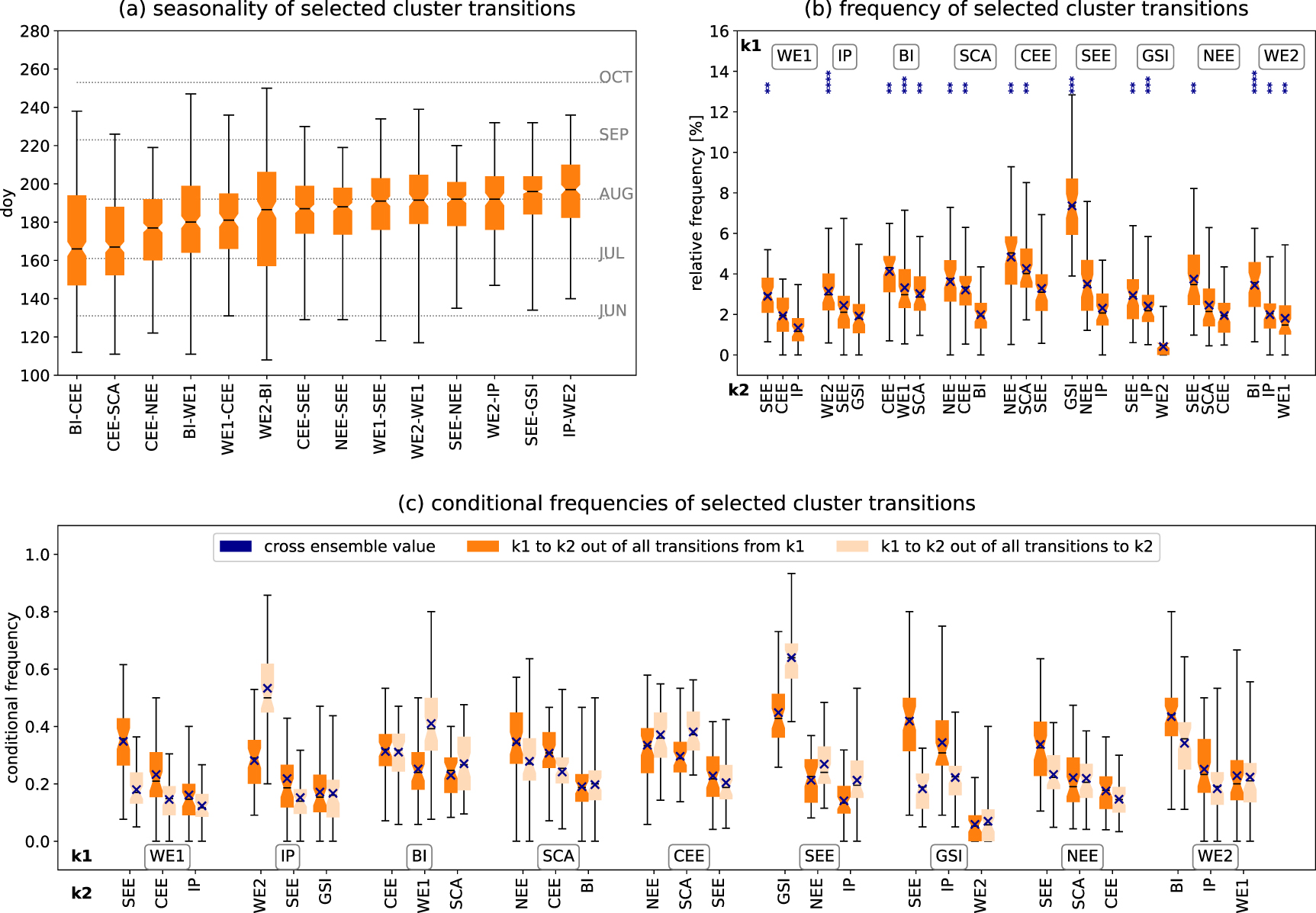
We next analyze pairs of core regions before and after transitions, i.e. the links derived in figure 3. All selected transitions occur most often during July and August (figure 4(a)); however, transitions in Western and North-Western regions tend to occur earlier (beginning of July) than South-Eastern regions (beginning of August) with the exception of transition IP–WE2. This is connected to the seasonal preference of heatwave clusters themselves (Felsche et al 2022).
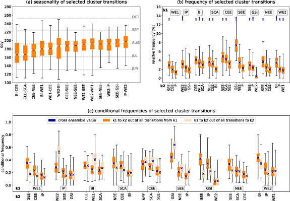
Figure 4. Transition characteristics: (a) seasonality of selected cluster transitions (day of the year) in CRCM5-LE. (b) Frequency of selected cluster transitions in 50 members of CRCM5-LE (boxplots) and pooled across the ensemble (crosses). Stars indicate the ratio of observed frequencies compared to expected frequencies under the assumption of k1 and k2 being independent. If this ratio is  2 we assume that independence can be rejected. (c) Selected cluster transitions expressed as conditional frequencies in 50 members (boxplots) and pooled across the ensemble (crosses). Light orange: frequency of k1 being followed by
  given that k1 is the first cluster in a pair (k1 and k2 being two different clusters, 1 and 2 indicating their position within a pair); orange: frequency of k2 being preceded by k1 given that k2 is the second cluster in a pair. For each first cluster subsequent clusters with top three highest conditional frequencies are selected in (b) and (c).
Download figure:
Standard image High-resolution imageThe links found in figure 3 are next evaluated against all possible links between the first and second cluster in a transition (k1 and k2). All of them rank among the top three most frequent transitions from their respective starting cluster (figures 4(b) and (c)). Transition occurrences of IP–WE2, WE2–BI and SEE–GSI, i.e. comparably short distances, exceed the expected value of randomly occurring transitions (i.e. k1 and k2 being independent) by factor 3 or 4. Among these, SEE–GSI mirrors source region–target region directions of trajectories found in Bieli et al 2015. The authors also identify trajectory source regions for heatwaves in the BI region west to Great Britain, which is not represented in figure 3. Generally, source regions (i.e. start regions in our analysis) of air masses are located close to heatwave occurrence regions (Bieli et al 2015).
Expressing transition strength in terms of conditional frequencies, figure 4(c) supports the results from the causal discovery network: Values of 1 would indicate a strict connection between both clusters, i.e. k1 is always followed by k2 and k2 being always preceded by k1. In other words, heatwave occurrence in k1 is likely a sufficient and necessary condition for heatwave occurrence in k2. Figure 4(c) shows high cross-ensemble values (and thus suggests strong connections) for, e.g. transitions SEE–GSI or IP–WE2, but also large variability among members: In 45% of all SEE occurrences, the heatwave propagates to GSI. Equally close connections characterize transitions WE2–BI (43%) or GSI–SEE (42%). This indicates a preference of heatwaves moving from the given first core region to the corresponding second core region within the analysis period.
3.2. Associated dynamic conditions
We next seek to connect these previously discussed transitions with potential drivers explaining their pathways (figure 5). Since negative soil moisture anomalies prevail before and after the transitions in the core regions (figure S3), we focus on centroid positions of positive Z500 anomalies during the two days preceding and two days following an indicated transition (figure 5). Our hypothesis states that a moving center of high pressure anomalies, as strong predictors of heat (Suarez-Gutierrez et al 2020), draws heatwaves with it in a similar direction. Acknowledging the fact that single events may deviate from these composites and the link between composites and heatwave occurrence may be not specific (Boschat et al 2016, Clemesha et al 2018, Zschenderlein et al 2019), we only examine regions where the signal exceeds the standard error among composite components. As was found for stationary heatwave patterns (Stefanon et al 2012), Z500 anomaly composites and temperature patterns correspond well in their spatial extent during transitions. Some heatwave footprints, however, are observed to be larger than their associated synoptic patterns (Spensberger et al 2020). The IP–WE2 Z500 and heat anomaly patterns as well as the propagation tracks are similar to the 'European Cluster' in Sánchez-Benítez et al 2020.

Figure 5. Z500 anomaly patterns (isolines) during four days preceding and following selected cluster transitions in CRCM5-LE (see Li et al
2020). Black circles with numbers indicate centroids of positive Z500 anomalies, colors highlight surface temperature anomaly composites during two days preceding and following cluster transitions. Blue triangles (crosses) mark centroid position of starting (ending) cluster footprint.  : frequency of indicated atmospheric pattern (AP) during given cluster transition (GT).
  : frequency of given cluster transition during indicated atmospheric pattern (among AP occurrences during any transition).
Download figure:
Standard image High-resolution image
In general, Z500 anomalies are located to the North-East of the heatwave core regions (compare crosses and triangles in figure 5). Blocking is known to intensify hot extremes southwest of its occurrence by various heating processes and advecting warm continental air masses (Pfahl 2014). For BI–CEE, CEE–SEE, BI–WE1, WE1–SEE, and SEE–GSI, centroid positions of Z500 anomalies lie between start and end positions of the transitions, in parts clearly mirroring the movement direction (see positions of 1–4 relative to each other, figure 5, and figure S3 for a comparison of selected links with CRCM5/ERA).
These associated patterns tend to appear during 12%–33% of the respective transitions in CRCM5-LE. Unsurprisingly, relative occurrences of the indicated transitions during all pattern occurrences remain low (0.1%–0.8%), given a high frequency of these patterns during May–October. Thus, the specific Z500 pattern occurrence is very likely not a sufficient cause for transition occurrence, but may be treated as a necessary condition (see Boschat et al 2016, Hannart et al 2016). Among pattern occurrence during any heatwave transition, however, the indicated transitions occur up to ten times more frequently, ranging from 2% to 7%. To summarize, associated pattern occurrence alone cannot be interpreted as a clear sufficient or necessary condition to causally explain heatwave transitions, although they tend to propagate in the same direction as contemporaneous heatwaves.
4. Discussion
By employing a framework involving causal discovery, we find indications of distinct heatwave tracks in Europe during 1981–2010. A very recent example of their meaningfulness is the July 2022 heatwave in Europe which started on the Iberian Peninsula, propagated towards Western Europe, Great Britain, Central-Eastern Europe and last to South-Eastern Europe (ECMWF 2022).
In parts, heatwave tracks are explained by large-scale circulation patterns (land-atmosphere or sea surface temperature related drivers were outside the study scope). Our approach allows to extract information on heatwave direction, dislocation velocity and seasonal occurrence along these tracks. These analyses are intended to understand a facet of spatially distributed extreme events, especially heatwaves, but not specifically to add to local prediction. Defining core regions based on naturally occurring geographical patterns of heatwaves rather than analyzing at arbitrarily chosen coordinates allows to perform a meaningful complexity reduction by grouping coherent spatial patterns to one core region. Causal discovery facilitates the comprehensive connection of heatwave regions across space and time and thus merges two dimensions which are commonly investigated separately. Moreover, it isolates dominant heatwave directional movements from a large dataset and identifies target regions of heatwave tracks.
Further investigation of recurrent heatwave tracks regarding the spatially varying interplay (Suarez-Gutierrez et al 2020) and importance of their respective drivers (as e.g. in Wu et al 2021) bears the potential to improve heatwave prediction or attenuation of regional driving factors by e.g. suitable land cover changes (Miralles et al 2019).
There are some limitations to our approach. First, employing a causal discovery algorithm requires certain conditions to be met (Spirtes and Glymour 1991, Ebert-Uphoff and Deng 2012a, Runge et al 2015): In order to correctly derive a network of directed links, all variables of relevance need to be included in the analysis (causal sufficiency). A spatially constrained domain may exclude regions of concern to the phenomenon. We attempt to evade this problem by constraining our analysis to land masses of Europe, i.e. heatwaves starting and ending in Europe. Moreover, large scale air mass flow—as shown to be related to heatwave tracks—dominantly follows a west-east path in Europe, thus leaving our domain towards the cut-off side. In order to clarify the influence of potentially missing nodes or variables outside the domain, we performed a leave-one-out analysis mimicking different 'domain sizes'. The analysis showed no considerable changes to the network (figure 3(b)). Thus, even if pathways entering/exiting the domain were missing, links within the domain would remain widely undisturbed. Consequently, the obtained links are valid with respect to the included nodes only as is also mentioned in Karmouche et al 2022.
This leads to the question why using a regional domain and not a global one, which may have avoided this problem. However, the selection of a small spatial domain reduced the risk of having several heatwaves with no common origin at the same time. Moreover, using a spatial resolution of 0.11∘ as opposed to, e.g. 1∘ or 2.8∘, leads to higher precision of spatial pattern delineation in heterogeneous landscapes (Molina et al 2020) and thus improves core region location.
Using a SMILE allows to derive a large variety of events and, consequently, of transitions among regions. This offers the opportunity to investigate likelihoods of links: For example, WE2–BI, SEE–GSI and CEE–NEE are more robust against the backdrop of internal variability than BI–CEE, CEE–SEE or NEE–SEE. Furthermore, in single realizations of reanalysis/observations long-lasting heatwaves may bias the clustering towards these events. For example, during the persistent 2010 heatwave in Russia, two clusters dominate (figure 2(b)), whereas clustering among 1500 rather than 30 years increases the likelihood of having various different spatial heatwave patterns as a baseline. Additionally, since heatwave tracks are extremely dependent on the exact weather patterns, small samples may bias expectations for larger samples. This was also found when investigating causal discovery links of single SMILE members (e.g. regarding CEE–SCA). Possibly large multi-model uncertainties (Nowack et al 2020) are beyond the scope of this study, but should be further investigated, e.g. in SMILEs of different models.
5. Summary and conclusions
In this study, we not only use causal discovery to derive observed spatio-temporal propagation of a phenomenon, but also to investigate spatio-temporal extremes on a more general ground for the first time in a SMILE. Thus the SMILE serves as a methodological testbed to investigate the power of causal discovery in abstracting spatio-temporal links from single event analyses. Additionally, we are able to infer that spatio-temporal links are represented plausibly in our SMILE which adds to common model evaluation based on static statistical metrics.
Causality in this study is understood as explaining the occurrence of heat anomalies at a given location by occurrences at more distant locations. Similar to established methods of heatwave tracking, our method is not confined to this type of spatial extremes and may be extended to investigate dominating landfall heatwave/drought paths.
We suggest that as high pressure anomalies propagate across Europe, associated high temperatures move along. Surface-atmospheric processes, e.g. moisture availability, evaporation, or heating of dry landscapes, may enhance or reduce temperatures, leading to a decoupling of Z500 and temperature anomalies after some time. A more detailed analysis of heat origins or temperature evolution during heatwaves (e.g. associated to Z500 timeseries) may extend the understanding of heatwave propagation. Further studies could also include investigations as to how heatwaves tracks and their connection to large-scale atmospheric patterns evolve under changing climate conditions or in different seasons. In order to verify model representation of heatwave tracks, we propose to repeat similar analyses in further (high-resolution) SMILEs. This could also help to better estimate the influence of domain choice.
If communicated broadly, recurring connections among core regions may foster awareness among people living in a downstream region whenever an upstream region is already affected by a heatwave.
Acknowledgments
This research was conducted within the ClimEx project (www.climex-project.org) funded by the Bavarian State Ministry for the Environment and Consumer Protection (Grant No. 81-0270-024570/2015). CRCM5 was developed by the ESCER Centre of Université du Québec à Montréal (UQAM; https://escer.uqam.ca/, last access: 16 August 2022) in collaboration with Environment and Climate Change Canada. The authors gratefully acknowledge the Leibniz Supercomputing center for funding this project by providing computing time on its Linux-Cluster. The authors would like to thank M Mittermeier, L Suarez Gutierrez and R Wood for discussions. The tigramite algorithm is provided via GitHub by J Runge.
Data availability statement
The data that support the findings of this study are available upon reasonable request from the authors.
Supplementary data (0.9 MB PDF)