

Abstract
To meet international and national commitments to decrease emissions of fossil fuels, cities around the world must obtain information on their historical levels of emissions, identifying hotspots that require special attention. Direct atmospheric measurements of pollution sources are almost impossible to obtain retrospectively. However, tree rings serve as an archive of environmental information for reconstructing the temporal and spatial distribution of fossil-fuel emissions in urban areas. Here, we present a novel methodology to reconstruct the spatial and temporal contribution of fossil-fuel CO2 concentration ([CO2F]) in the urban area of Medellin, Colombia. We used a combination of dendrochronological analyses, radiocarbon measurements, and statistical modeling. We obtained annual maps of [CO2F] from 1977 to 2018 that describe changes in its spatial distribution over time. Our method was successful at identifying hotspots of emissions around industrial areas, and areas with high traffic density. It also identified temporal trends that may be related to socioeconomic and technological factors. We observed an important increase in [CO2F] during the last decade, which suggests that efforts of city officials to reduce traffic and emissions did not have a significant impact on the contribution of fossil fuels to local air. The method presented here could be of significant value for city planners and environmental officials from other urban areas around the world. It allows identifying hotspots of fossil fuels emissions, evaluating the impact of previous environmental policies, and planning new interventions to reduce emissions.
Export citation and abstract BibTeX RIS

Original content from this work may be used under the terms of the Creative Commons Attribution 4.0 license. Any further distribution of this work must maintain attribution to the author(s) and the title of the work, journal citation and DOI.
1. Introduction
Annual tree rings can be used to spatially reconstruct historical levels of particular chemical properties of air such as the concentration of heavy metals, radioactive elements, and other polluting compounds. Through photosynthesis, trees fix 12C (98.89%), 13C (1.11%), and 14C (10−10%) from atmospheric CO2 and use this carbon to produce tree-ring wood. During a particular year, 14C used to produce tree-ring wood can be considered analogous to the 14CO2 in the atmosphere at the time of fixation (Worbes 1999, Dongarrà and Varrica 2002, Pataki et al 2010, Sensuła and Pazdur 2013). The burning of fossil fuels has been the main source of increase in atmospheric CO2 in the previous decades (Friedlingstein et al 2021). Fossil fuels are devoid of 14C; for this reason, their emissions reduce the 14CO2 to 12CO2 ratio, allowing one to obtain estimates of the contribution of fossil fuel burning to the local air (Levin et al 1989, Turnbull et al 2016). Thus, the difference in the isotopic concentration of air from a clean area versus air from urban or industrial areas can be used to calculate the percentage contribution of CO2 derived from fossil fuels (Djuricin et al 2012, Turnbull et al 2016). This phenomenon is known as the Suess effect (1955) or dilution effect of atmospheric 14C in polluted areas (Levin et al 1989).
Previous studies have demonstrated the utility of tree ring analyses and 14C measurements to temporally reconstruct fossil-fuel emissions in different cities around the world (Cain 1978, Rakowski et al 2001, 2004a, 2004b, 2008, 2013, Pazdur et al 2007, Battipaglia et al 2010, Capano et al 2010, Beramendi-Orosco et al 2013, 2015, 2018, Ješkovský et al 2015, Xu et al 2015, 2016, Flores et al 2017, Kontuľ et al 2017). These previous studies have shown clear differences in 14C values between remote areas with clean air, and densely populated areas with larger industrial and traffic footprints, corresponding to more polluted atmospheres. However, probably due to the high cost of radiocarbon analyses, most studies only provide a snapshot of the contribution of fossil fuels in urban environments. More comprehensive spatial and temporal reconstructions spanning several decades, and different city environments still have to be done to demonstrate the high potential of this method for the design or evaluation of policies aiming at reducing emissions of fossil fuels.
One advantage of tree rings, compared to other studies based on the direct atmospheric sampling of 14CO2, is that trees can be sampled multiple times over a large spatial domain. Therefore, the history of emissions in urban environments can be reconstructed in space and time. With these considerations in mind, we designed a study to address the question: Can we reconstruct, in time and space, the fossil fuel CO2 concentrations [CO2F] in the urban area of Medellín (UAM), Colombia, using dendrochronological and isotopic methods? Therefore, our objectives were to (a) develop a statistical model to reconstruct [CO2F] in space and time using dendrochronology and radiocarbon methods, (b) characterize the changes in [CO2F] that have occurred spatially and temporally in a large urban area with significant population growth, and (c) discuss possible factors that have induced changes in [CO2F] in space and time. Our a priori expectations were that the spatial and temporal reconstruction method identifies different zones, such as residential, with low vehicular flow, and industrial, with high contributions of emissions that dilute the local 14CO2 air.
2. Materials and methods
2.1. Study area
This study was conducted in the UAM, Colombia, a South American city located in the northern part of the Andean Mountains, from 6°17'40'' to 6°11'58''N, and from 75°17'40'' to 75°32'56''E. The city has a mean annual temperature of 21.6 °C, and mean annual precipitation of 1612 mm. January is the driest month with 52 mm on average, and October is the wettest, with 207 mm on average. The mean altitude is 1475 m. The city's inhabitants are currently above 2.5 million and have increased in previous decades due to massive immigration from other parts of Colombia and Venezuela.
2.2. Dendrochronological analysis
2.2.1. Sampling
Thirty-five urban trees of Fraxinus uhdei, located across the UAM, were sampled using an increment borer by taking three cores from each tree. We selected healthy trees located along major streets, excluding trees with evidence of excessive pruning or symptoms of diseases or plagues. The core samples were mounted on prefabricated wooden supports, dried for 12 h at 35 °C, and sanded with increasing grit number sandpaper (60–1200) to improve visualization of wood anatomy. Each core was scanned at 1800 dpi using an Epson Expression 10000XL scanner, calibrated by Regent Instruments from Canada for dendrochronological studies. Tree rings were marked within 0.014 mm accuracy using the ImageJ program (Schneider et al 2012). Tree-ring widths (TRWs) were measured on the scanned images using a script programmed using the R statistical environment (R Core Team 2020). The script processes points in the scanned images selected with the selection tools of ImageJ and computes the Euclidean distance between selected points.
2.2.2. Crossdating
The quality of the dates assigned to the TRWs was controlled by cross-dating (Douglass 1941, Speer 2010). This technique allowed us to identify the exact year in which each tree ring was formed and served as statistical control for the visual identification of the TRWs. The cross-dating consisted of comparing the TRW series within the same tree and between different trees using different parametric indicators (Douglass 1941, Speer 2010). Cross-dating was carried out with the R package dplR (Dendrochronology Program Library) (Bunn 2008) using functions to calculate signal-to-noise ratio (SNR), expressed population signal (EPS), and the mean sensitivity (MS) according to methods described in Cook and Kairiukstis (1990).
2.3. Radiocarbon analysis
2.3.1. Determination of radiocarbon
We extracted the α-cellulose from a complete core from each sampled tree. Then, by comparing the core after α-cellulose extraction with the other core replicates of the same tree, we extracted α-cellulose samples for 14C analysis of one out of every four rings and assigned the corresponding calendar year. From each ring, we extracted about 30 mg from latewood α-cellulose. Earlywood was disregarded because it may contain some cellulose of non-structural photosynthetic products from previous years stored in the parenchymal wood tissue. A total of 282 samples were analyzed for 14C, which on average is equivalent to eight rings per tree. We extracted the α-cellulose in a Soxhlet system at the Laboratory of Agro-industrial Processes of the Universidad Pontificia Bolivariana in Medellín. This laboratory followed the protocol established by Durgante (2017) to control biases in the radiocarbon analyses due to contamination of the sampled cellulose; the process used ethanol- and toluene-based solutions for extracting lipids from wood. Then, the samples were bleached with sodium hypochlorite and acetic acid. Then, the α-cellulose was extracted by sodium hydroxide and acetic acid. The radiocarbon concentration of the extracted α-cellulose was measured using accelerator mass spectrometry at the Max Planck Institute for Biogeochemistry in Jena, Germany (Steinhof et al 2017).
2.3.2. Calculation of the CO2 concentration of fossil fuel origin [CO2F]
Concentrations of fossil fuels [CO2F] (ppm) were estimated processing the radiocarbon concentration data and combining two mass balance equations (Levin et al 1989, 2003) to obtain the following formula (see mathematical derivation in supplementary material 1 available online at stacks.iop.org/ERL/17/055008/mmedia)
where ![$\left[ {{\text{CO}_2 \text{F}}} \right]$](https://content.cld.iop.org/journals/1748-9326/17/5/055008/revision2/erlac63d4ieqn1.gif) is the estimated mole fraction, in ppm, of CO2 derived from fossil emission sources;
is the estimated mole fraction, in ppm, of CO2 derived from fossil emission sources; ![${\left[ {{\text{C}}{{\text{O}}_{\text{2}}}} \right]_{{\text{BG}}}}$](https://content.cld.iop.org/journals/1748-9326/17/5/055008/revision2/erlac63d4ieqn2.gif) is the atmospheric CO2 mole fraction in the background area;
is the atmospheric CO2 mole fraction in the background area;  and
and  are the 14C isotopic ratio (in ‰) for the background air and for the measured sample at the UAM, respectively. As the
 ![${\left[ {{\text{C}}{{\text{O}}_2}} \right]_{{\text{BG}}}}$](https://content.cld.iop.org/journals/1748-9326/17/5/055008/revision2/erlac63d4ieqn5.gif) has not been measured in the background area, we assumed it corresponds to the annual mean values reported for the Mauna Loa station in Hawai'i, assuming it represents global clean air (Tans and Kirk 2018). For the
has not been measured in the background area, we assumed it corresponds to the annual mean values reported for the Mauna Loa station in Hawai'i, assuming it represents global clean air (Tans and Kirk 2018). For the  , we used
  data from the Northern Hemisphere Zone 3 curve (Hua et al
2021), corresponding to the time-span from 1977 to 2018.
data from the Northern Hemisphere Zone 3 curve (Hua et al
2021), corresponding to the time-span from 1977 to 2018.
2.3.3. Comparison with official reports of CO2 emissions
The [CO2F] values in ppm were compared with official UAM CO2 emission records (in Tg C yr−1) (Toro et al 2013, 2015, 2017, 2018). [CO2F] values were averaged, according to the temporal resolution of the CO2 emission records obtained (2000–2017). A linear regression model was fitted between [CO2F] and the records of CO2 emissions to evaluate the degree of agreement between the [CO2F] concentration values and the total emission values.
2.4. Time—series analysis
Since [CO2F] was calculated from radiocarbon analyses at discontinuous time steps, [CO2F] values for the years studied were estimated using a mixed-effects model that predicts [CO2F] as a function of time and quantifies random effects on the model parameters. Preliminary analyses of the scatter plots of [CO2F] over time indicated polynomial patterns in all trees with deviations in residual variance due to core variability. Therefore, in the mixed model, the effect of each core on the polynomial trend of the series was considered as follows:
where numeric subscripts indicate fixed effects, alphabetic subscripts (s) indicate random effects at tree level, t is time (yr); es,t is a vector of normalized residuals, Rs is the variance-covariance matrix of the residuals. The variables time (t) and [CO2F] were fitted as fixed effects and the tree as random effects. Improvements in the model by accounting for tree variability were measured using Akaike's Information Criterion (AIC) and maximum likelihood ratio-tests between the mixed-effects model and an equivalent equation without random effects (Pinheiro and Bates 2000). This mixed-effects model was fitted with the nlme (Linear and Nonlinear Mixed Effects Models) package (Pinheiro et al 2021) of the R software.
2.5. Spatial analysis
Here we assume that the spatial distribution of [CO2F] across the UAM is mainly related to the trees' location, and that the effects from other biophysical processes are negligible. This assumption allowed us to interpolate contours of [CO2F] over the spatial domain. Spatial interpolation plots of [CO2F] in the UAM were established for five-year windows from 1980 to 2015, and for 2018 (the last year sampled). We used inverse distance weighting (IDW) (Legendre and Legendre 2012); a method based on the assumption that data with closer spatial proximity are more closely related than the more distant (Spokas et al 2003). Since the number of values to interpolate defines the quality of interpolation, the resulting contours are completely representative of the series. Spatial interpolation was established using R libraries for spatial analysis, including sp, raster (Bivand et al 2013), and rgeos (Bivand et al 2017).
We also estimated the uncertainty in the spatial interpolations by computing a map of standard deviations between 1980 and 2018 across the study site. First, we derived annual contour plots between 1980 and 2018 using the mixed-effects model and the IDW. Second, we derived the uncertainty map by plotting the standard deviation estimates for each pixel position.
3. Results
3.1. Dendrochronological analysis
The average period for the TRWs ranged from 1977 to 2018. Statistical parameters obtained during the cross-dating process confirmed the annual periodicity of the tree rings of F. uhdei (see supplementary material 2). A total of 964 tree rings were measured. The mean TRWs was 6.196 mm, and the Gini coefficient was 0.23. The overall running  was 0.41 (p < 0.05). The mean first-order autocorrelation was −0.06, the EPS was 0.96, and it exceeds the threshold of 0.85 since 1988 (Speer 2010). The MS was 0.43, and the SNR was 24.32. The residual TRW chronology is presented in the supplementary material 3.
3.2. Temporal patterns in radiocarbon and [CO2F]
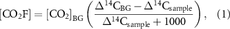
Mean radiocarbon concentrations (Δ14C) for all trees in the UAM between 1977 and 2018 were lower than the corresponding concentrations for the background air (figure 1). The observed data showed radiocarbon dilution (Suess effect), particularly strong for the last part of the curve, between about 2011 and 2018.
Figure 1. Radiocarbon concentration in the background air and in the measured tree rings expressed as Δ14C (‰) over time. The red dots indicate the annual concentrations measured in the tree rings of Fraxinus udhei from the urban area of Medellín (UAM). The black line represent the background 'clean air' concentration obtained from the North Hemisphere Zone 3 (NH3) curve.
Download figure:
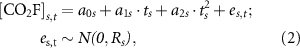
Standard image High-resolution imageThe computed [CO2F] values showed high variability during the 41 years recorded by tree rings (figure 2). High values of [CO2F] occurred between 1977 and 1987. However, during this period, a small sample size of 14C measurements were obtained with only one ring per year in 1977 and 1978, or between 2 or 3 rings per year; hence the observed high standard deviations. Then, between 1986 and 2012 [CO2F] values remained relatively stable; but from 2013 to 2018, they grew consistently reaching the highest observed values (figure 2). High variability in [CO2F] is likely due to differences in CO2 emission sources at different locations, which motived the spatial analysis presented in section 3.5.
Figure 2. The concentration of fossil fuel CO2 [CO2F] values over time in ppm for the urban area of Medellín between 1977 and 2017. The vertical bars indicate the standard deviation between tree rings. Numbers above the bars indicate the sample size for 14C analyses.
Download figure:
Standard image High-resolution image3.3. Comparison with emission data
The obtained [CO2F] values compared relatively well with official CO2 emission data reported for the UAM (figure 3). Both the intercept and the slope of the linear model between the two variables were highly significant (p < 3.7 × 10⁻⁵). The coefficient of determination was 0.67. The obtained scatter plot exhibited some variability, with a higher density of points between 2000 and 2012 (figure 3). Although the remaining 5 years are represented by a lower point density, they spanned the entire regression domain, ensuring good confidence of the model parameters for at least the last 17 years of the study.
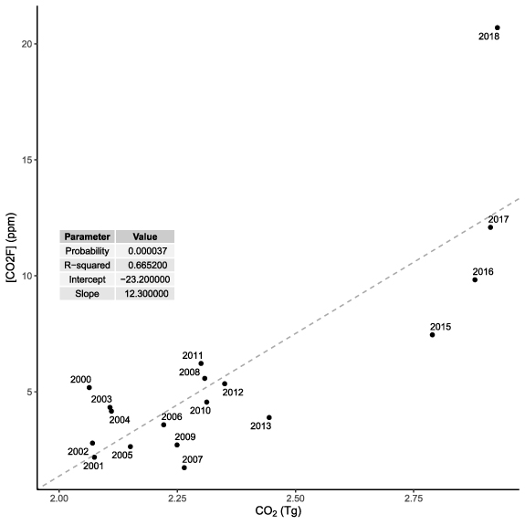
Figure 3. Comparison between average values of the concentrations of fossil fuel calculated in this study and official CO2 emission data for the urban area of Medellín reported in official reports during the years 2000–2017.
Download figure:
Standard image High-resolution image3.4. Time-series analysis
Fixed-effect parameters of the mixed model confirmed the polynomial trend of [CO2F] over time (table 1, p-values). Although the a0 parameter was not significant, the other two parameters indicated a parabolic trend. The regression fitted by the mixed-effects model shows upward concave quadratic behavior in the 35 trees sampled. For most trees (figure 4), interpolations show that [CO2F] values have decreased since the 1980s; they reached minimum values around the year 2000, and then increased until 2018. The importance of accounting for the tree-effect in the model is better appreciated by the difference in AIC values between the mixed model (AIC = 1419.801) versus the model without random effects (AIC = 1504.542), which differed significantly (Likelihood ratio = 96.741, p < 0.001) (table 2). In addition, the residual standard deviation of the mixed model with random effects (table 1, random effects sd = 2.336) was much smaller than that of the model without random effects (sd = 3.455).

Figure 4. Predictions of the mixed-effects model and tree-ring based estimates of the concentrations of fossil fuel CO2 [CO2F] over time. Each number indicates the tree code and correspond to the locations presented in figure 5.
Download figure:
Standard image High-resolution imageTable 1. Parameter estimators of the mixed-effects model for the fossil-fuel CO2 concentrations over time. The variables time and [CO2F] represent the fixed effects, and the trees the random effects.
| Fixed effects | Value | Standard error | t-value | p-value |
|---|---|---|---|---|
| a0 | 5.584 | 0.354 | 15.759 | 0.000 |
| a1 | 9.978 | 5.033 | 1.983 | 0.049 |
| a2 | 39.763 | 4.851 | 8.197 | 0.000 |
| Random effects | StdDev | Correlation | ||
| a0s | 1.826 | — | — | — |
| a1s | 21.754 | −0.414 | — | — |
| a2s | 20.241 | 0.130 | — | — |
| Residual | 2.336 | — | — | — |
Table 2. ANOVA to compare the mixed-effects model (M1) and an equivalent model with no random effects (M0).
| Model | df | AIC | BIC | logLik | L.Ratio | p-value |
|---|---|---|---|---|---|---|
| M1 | 10 | 1419.801 | 1456.22 | −699.900 | — | — |
| M0 | 4 | 1504.542 | 1519.11 | −748.271 | 96.714 | <.0001 |
In most trees, the quadratic function estimates a reduction of [CO2F] in tree rings during the 1980s and 1990s. They reach minimum values around the year 2000 and then increased consistently until 2018 (figure 4).
3.5. Spatial analysis
The spatial distribution of [CO2F] in the UAM for a set of selected calendar years showed that fossil fuel emissions are not distributed homogeneously over the UAM. Some locations of the city have changed differently over time, with the highest values of [CO2F] observed for the selected years 1980, 2015, and 2018 (figure 5, blue gradient). The lowest [CO2F] values occurred between 1995 and 2000 (figure 5, yellow-green gradient). Overall, the downtown area depicted at the center of the panels always had the highest [CO2F] values (figure 5). Our space-time method revealed two hotspots of high [CO2F] concentration in the UAM and their evolution between 1980 and 2018. One around downtown, and another to the south (figure 5, left). Similarly, and in agreement with the previous time series analysis, we observed that the temporal evolution of [CO2F] consistently decreased from 1980 to 2000 across the entire domain, and then consistently increased again until the last year of observation in 2018.
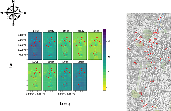
Figure 5. Spatial interpolation of fossil fuel concentrations [CO2F] (scalebar in ppm) across the urban area of Medellín, in five-year windows between 1980 and 2015 and for the year 2018; the red dots in each window represent the location of the 35 trees of F. uhdei. The panel on the right represents the UAM for the year 2020. Red dots are the 35 sampled trees with their respective code.
Download figure:
Standard image High-resolution imageWhen we observe the UAM road mesh (figure 5, right), several hotspots of high pollution of [CO2F] (light green color, about 5 ppm) appear towards the downtown, north, and south. The main streets and avenues also present high pollution (light green color, about 5 ppm) and even higher values (blue color, about 15 ppm).
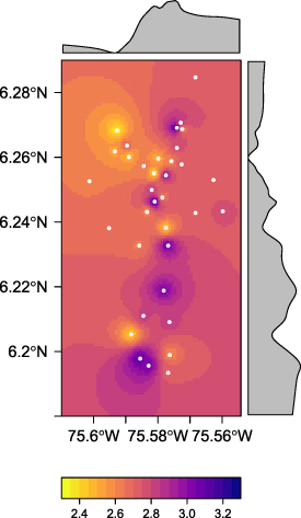
The uncertainties are in the range of 2.4–3.2 ppm (figure 6), most of the uncertainties are less than 3 ppm. The points of greatest variability are defined by tree locality. There are seven trees that are contributing the highest variability, which are mostly clustered around the downtown area of the UAM.
Figure 6. Uncertainty map of spatial interpolations of fossil fuel concentrations [CO2F] (scale bar in ppm) across the urban area of Medellín, between 1980 and 2018; the white dots represent the location of the 35 trees of F. uhdei.
Download figure:
Standard image High-resolution image
4. Discussion
This study demonstrated the utility of radiocarbon analyses in annual tree rings to reconstruct the spatial and temporal contribution of fossil fuels to the atmosphere of a city. It confirms the existence of annual rings in F. uhdei (Villanueva Díaz et al 2015) outside its natural distribution range, and demonstrates its usefulness to study pollution by fossil fuels in cities, previously reported only for Mexico (Beramendi-Orosco et al 2013).
An important novel aspect of our study is the use of a mixed-effects model, which allowed us to interpolate the [CO2F] in years where we did not analyze 14C, controlling for the variance of individual trees that are subject to specific levels of urban pollution. Our method allowed us to reconstruct spatially and temporally the mean values of [CO2F] for 41 years at an annual resolution (figure 5), with a robust quantification of prediction uncertainty (figure 6), which is a measure of the variability due to (a) variability of atmospheric 14CO2 values, and (b) uncertainty in ring growth and dating.
High variability in 14CO2 can be attributed mainly to the heterogeneity of emission sources within the urban environment, and to a lesser degree to atmospheric transport from the Northern hemisphere through the dynamics of intertropical convergence zone (ITCZ) (Ancapichún et al 2021, Hua et al 2021). In South America (SA), the ITCZ migrates annually from January to July from southern Brazil and northern Argentina towards the north. From July to January it returns to the south. However, it leaves SA to the west through a narrow strip in the Pacific coast (Ancapichún et al 2021). This region of ITCZ activity exactly coincides with the SA domain of the Northern Hemisphere Zone 3 curve (Hua et al 2021) used in this study. The mean position of the ITCZ, where low pressures are present throughout the year, is located at about 4–5° N on the Colombian Pacific coast (Ancapichún et al 2021). Medellin, at about 6.2° N, is influenced by the ITCZ twice a year. Therefore, both winds from the southeast Amazon basin and from the northeastern savannas of Venezuela transport air to Medellín. The 14C NH Zone 3 curve (Hua et al 2021) captures well these different sources of 14CO2 in the background air.
Another source of variability in [CO2F] can be explained by variability due to tree-ring growth and uncertainties in tree-ring dating. In the urban environment, there is a large heterogeneity in the conditions in which individual trees grow, with some trees under high stress imposed by physical barriers (e.g. cement and asphalt). In contrast, in open areas without water and light limitation, trees tend to develop complacent rings that, even when well-dated, have low correlations with the mean chronology. In addition, during their development phase, the trees grew in a nursery within the city. Their subsequent transplant to their final location may affect the values of [CO2F] during the first few years of the chronology.
Our quantification of uncertainty in the predictions (figure 6) captures these differences sources of variability and helps to identify hotspots of variability in [CO2F]. The uncertainty values of [CO2F] that we obtained are of only a few ppm and suggest that the different sources of uncertainty mentioned in the previous paragraphs contribute only a small proportion to the total uncertainty in predictions.
The parabolic patterns revealed by the [CO2F] values and captured by the model are challenging to interpret (figures 4 and 5). They could be explained by numerous reasons ranging from changes in the local distribution of emission sources to global economic factors affecting oil prices and local consumption. Between 1980 and 2000, the population of Medellin grew from about one to about two million people, and both the fixed and mobile sources of CO2 of the UAM increased (Toro et al 2013, 2015, 2017, 2018, 2019). Why then did the [CO2F] values decrease from 1977 to 1985? One potential explanation may have to do with the small number of observations for the early years in our record. Another possible explanation for the high [CO2F] values found early in the record may be related to the elevated industrial activity during this period.
The decrease in [CO2F] values from 1990 to 2000 might be related to the withdrawal of heavy industries from the UAM. This is the case of the metallurgic company Siderúrgica de Medellín and the Argos cement plant as well as other heavy industries (Molina 2013). From this industrial area emerged a residential area with parks and museums. At the end of 1995, the Medellín Metro was inaugurated, providing a massive scale transportation system. During the 1990s, the transition from the carburetor to injection systems began in most engines, possibly increasing efficiency in fuel consumption.
In contrast, from 2000 to 2018, the [CO2F] increased considerably (figures 4 and 5), which was expected due to a large increase in population, which grew from about two million in 2000 to about 2.5 million in 2018, accompanied with an increase in the vehicle fleet. No local policies managed to bend the upward curve of [CO2F] in the last decades, namely: restrictions of mobility adopted by the city in 2001, the expansion of the Metro (2004, 2008, and 2016), or the implementation of the transport system with cables and electric trams.
5. Conclusions
By using a combination of dendrochronological analyses, radiocarbon measurements in tree rings, and statistical modelling, we were able to reconstruct spatially and temporally the contribution of fossil fuel carbon to the atmosphere of the urban area of Medellin, Colombia. This reconstruction, which spans from 1977 to 2018, identified hotspots of emissions related to traffic and industrial areas as well as urban population growth. We identified an increase in the contribution of fossil fuel carbon to atmospheric CO2 in the last decades, and recent efforts from local authorities to reduce traffic and emissions do not seem to have a distinguishable effect on [CO2F]. The method we developed here could be of tremendous utility for reconstructing the history of fossil fuel emissions in many other cities and identify hotspots. This method provides valuable information for the planning and evaluation of measures to reduce emissions in urban areas.
Acknowledgments
We thank the Max Planck Institute for Biogeochemistry in Jena, Germany, and Minciencias, Colombia (Project Code: 39934), for financial support. We are also grateful to contributions by the members of the Laboratory of Tropical Dendroecology of the Universidad Nacional de Colombia-Medellín, and D Herrera-Ramírez for logistic support.
Data availability statement
The data that support the findings of this study are openly available at the following URL/DOI: https://doi.org/10.5281/zenodo.6443402. Data will be available from 01 March 2022.