

Abstract
In the context of 100% renewable electricity systems, prolonged periods with persistently scarce supply from wind and solar resources have received increasing academic and political attention. This article explores how such scarcity periods relate to energy storage requirements. To this end, we contrast results from a time series analysis with those from a system cost optimization model, based on a German 100% renewable case study using 35 years of hourly time series data. While our time series analysis supports previous findings that periods with persistently scarce supply last no longer than two weeks, we find that the maximum energy deficit occurs over a much longer period of nine weeks. This is because multiple scarce periods can closely follow each other. When considering storage losses and charging limitations, the period defining storage requirements extends over as much as 12 weeks. For this longer period, the cost-optimal storage needs to be large enough to supply 36 TWh of electricity, which is about three times larger than the energy deficit of the scarcest two weeks. Most of this storage is provided via hydrogen storage in salt caverns, of which the capacity is even larger due to electricity reconversion losses (55 TWh). Adding other sources of flexibility, for example with bioenergy, the duration of the period that defines storage requirements lengthens to more than one year. When optimizing system costs based on a single year rather than a multi-year time series, we find substantial inter-annual variation in the overall storage requirements, with the average year needing less than half as much storage as calculated for all 35 years together. We conclude that focusing on short-duration extreme events or single years can lead to an underestimation of storage requirements and costs of a 100% renewable system.
Export citation and abstract BibTeX RIS

Original content from this work may be used under the terms of the Creative Commons Attribution 4.0 license. Any further distribution of this work must maintain attribution to the author(s) and the title of the work, journal citation and DOI.
1. Introduction
The viability of 100% renewable electricity supply continues to be a controversial topic (Jacobson et al 2015, Clack et al 2017, Heard et al 2017, Brown et al 2018, Bogdanov et al 2019, Tröndle et al 2020). Because a fully renewable electricity system must heavily rely on wind and solar energy in most countries, one frequently discussed aspect is the system reliability during events with low availability of these variable energy sources. For the example of Germany, such extreme events have also received public and political attention (Wetzel 2019, German Federal Government 2021), and the German term for dark doldrums, Dunkelflaute, has made it to the international debate (Li et al 2020, 2021, Ohlendorf and Schill 2020, de Vries and Doorman 2021).
Previous studies on renewable scarcity periods mostly focused on wind energy (Cannon et al 2015, Patlakas et al 2017, Ohlendorf and Schill 2020). These studies are similar in their approaches and results. They define a threshold below which wind power or wind speed is considered 'low'. On this basis, they characterize the frequency and duration of low-wind periods based on decades-long, national time series. The maximum duration of low-wind events identified in these studies is 4–10 d (see appendix table A1 for details).
Further time series analyses found that, due to geographical smoothing, low-wind events are more pronounced when focusing on single locations (Leahy and McKeogh 2013) and become less extreme when extending the geographical scope to the continental scale (Grams et al 2017, Handschy et al 2017, Kaspar et al 2019). Finally, Raynaud et al (2018) extended the scope to solar, hydro, and load to examine 'energy droughts', defined as periods when renewables supply less than 20% of demand. They found that a mix of renewables reduces the duration of energy droughts by a factor of two or more when compared to single energy sources, and that the duration of energy droughts will not exceed 2 d in 100% renewable scenarios. While several studies claimed that the identified scarcity periods will define storage requirements in renewable electricity systems, it remains unclear whether and how storage requirements can be inferred from the results.
Meanwhile, many studies have analyzed the cost-optimal configuration of 100% renewable electricity systems (see Hansen et al (2019) for a review). These studies employ optimization models to decide on the investment in renewable generators and energy storage, solving the trade-off between storage and renewable curtailment (Zerrahn et al 2018). Besides storage, the models usually consider other flexibility options such as flexible supply from bioenergy, demand response, and international electricity trade. The results of five German and European studies are summarized in the appendix (table A2). The reported optimal storage energy capacities are large enough to supply 12–32 d of the average load within the considered region, which is about 2–3 times longer than what time series analyses found as the duration of low-wind events.
Contrasting the results from time series analyses and optimization models seems interesting for three reasons. First, the larger storage volumes 3 in the optimization studies suggest that storage requirements may not directly be inferred from the length of the worst Dunkelflaute as identified by time series analyses. Second, the larger storage volumes in the optimization studies seem counter-intuitive given that these studies include flexibility options beyond storage, which are not considered in the times series analyses. Third, the above optimization models are based on 1–3 weather years, and it remains unclear whether these years include the worst Dunkelflaute periods as identified by the time series analyses based on multiple-decades-long datasets. While previous studies analyzed the inter-annual variability of renewables and implications for system planning in general (Pfenninger 2017, Collins et al 2018, Schlachtberger et al 2018, Zeyringer et al 2018, Kumler et al 2019), the implications for storage energy requirements in particular remain unclear. A notable exception is a study by Dowling et al (2020), which relates long-term storage requirements to the inter-annual variability of renewables but without analyzing the role of extreme events.
This study bridges the gap between time series analyses of extreme events and optimization models. On the one hand, we analyze 35 years of renewable and load time series to characterize the Dunkelflaute in terms of the maximum energy deficit accumulating over a certain period. We also calculate the required storage energy capacity with a stylized cost optimization model using the same input time series. The role of other flexibility options on storage requirements is analyzed using the example of flexible bioenergy. Finally, we contrast the optimization results based on single versus multiple years of data.
Our work contributes to the understanding of how the variability of renewable sources defines storage requirements in a 100% renewable electricity system. Our findings suggest that both time series analyses and optimization models often come with simplifications that may lead to an underestimation of storage requirements. Regarding time series analyses, it appears insufficient to look at short periods with extreme scarcity because these can be surrounded by other scarcity periods, which jointly define storage needs. Regarding optimization models, analyzing single years seems insufficient because these do not necessarily include extreme events. Furthermore, with an increase in other flexibility options, the role of long-term storage transitions from bridging extreme events to smoothening the inter-annual variability of renewables.
The remainder of this paper is structured as follows. Section 2 describes the applied methods and utilized data, section 3 presents the results, section 4 discusses the findings, and section 5 draws conclusions.
2. Methods and data
This section describes the time series data (section 2.1), which serve as an input to the subsequently introduced optimization model (section 2.2) and time series analysis (section 2.3). To highlight methodical similarities and differences, we use rather stylized assumptions—the limitations of which are discussed in section 4.
2.1. Time series data
Both methods use 35 years-long time series data from the European Network of Transmission System Operators for Electricity, ENTSO-E (2020) as an input. These time series reflect a scenario for 2030 based on weather reanalysis data from 1982 to 2016. This dataset is used by European system operators for adequacy calculations and, more generally, reanalysis data have frequently been used in the literature on renewable electricity systems (Cannon et al 2015, Ohlendorf and Schill 2020, Tröndle et al 2020, Neumann and Brown 2021). The dataset includes hourly load data and hourly generation profiles for wind and solar energy at the national level. Furthermore, daily generation time series are provided for hydro run-of-river (hydro ROR), as well as weekly time series for the natural inflow to hydro reservoirs and to pumped hydro storage.
Being based on a scenario for the year 2030, these time series reflect some changes that can be expected compared to current observations. For example, the load profiles account for the expected increase in electric vehicles and heat pumps by 2030, and generation profiles reflect the expected distribution and technology of wind and solar power plants in 2030. It should be noted, however, that a potential 100% renewable electricity system may only be reached toward 2050. The load and generation profiles may exhibit further changes by then, as discussed in section 4.
2.2. Cost optimization model
We use an optimization model to find the least-cost 100% renewable electricity system for the example of Germany. The model decides on investment in variable renewable generators and electricity storage in batteries and via hydrogen. Simultaneously, the dispatch of storage is optimized, while considering existing bioenergy and hydro power (including pumped hydro storage). The optimization problem extends over 35 consecutive years with an hourly resolution of dispatch. For every hour, primary renewable electricity supply plus storage discharging minus storage charging and curtailment must be equal to load at the country level. The storage level at the beginning of each year is determined by the model but must be equal to the storage level at the end of the previous year. For perspective, further model runs are conducted based on single years, and the results are contrasted with those of the multi-year optimization (section 3.5).
The investment variables for variable renewables include three distinct technologies: solar photovoltaic (PV), onshore wind, and offshore wind. The investment in batteries is distinguished into an energy-specific component (the battery packs) and a power-specific component (the inverters). For hydrogen storage, three investment dimensions are considered: energy (salt caverns), charging power (electrolyzers), and discharging power (combined cycle gas turbines, CCGTs). The annualized investment costs and the fixed operation and maintenance costs for all these technologies are included in the objective function of the optimization model.
The hourly dispatch optimization is based on the time series data described in section 2.3. Load time series are used as is, and the generation profiles for wind and solar energy are scaled according to the corresponding investment variables. Put differently, the per-MW renewable profiles are multiplied with the installed capacity as determined by the cost optimization model. Hydro ROR is fixed to the provided daily time series, with the hourly generation being constant throughout the days. Reservoir and pumped hydro are modeled as one generic dispatchable hydro technology (hydro DIS), considering the weekly inflow profiles and constraints imposed by existing capacity. For comparability with the time series analysis, bioenergy is conservatively assumed to produce at constant load in the base case, and a more flexible operation is considered in a sensitivity analysis (section 3.4).
The cost optimization model is described in detail in the appendix
2.3. Time series analysis
Based on the time series data described in section 2.3, we define the maximum energy deficit as follows:
with:
where  and
and  are start and end timestamps of the period with the maximum energy deficit.
  is the hourly load data and
  is the sum of renewable electricity generation. For wind and solar energy,
  ,
,  , and
, and  are outputs of the cost optimization model. The generation of hydro ROR
  is based on the input time series described in section 2.1, and for hydro reservoirs and pumped storage, the natural inflow
  is considered. Hence, we are calculating a gross deficit in the sense that available storage capacity of hydro power is not yet deducted. Bioenergy is assumed to produce at a constant load to make the results of the time series analysis and of the cost optimization model comparable. To identify the overall maximum energy deficit,
  and
and  are two independent arguments of the maximization algorithm with
  . In addition, we compute the maximum energy deficits for different durations
  . The resulting periods for the maximum energy deficits with different durations can possibly but not necessarily overlap (see section 3.2 below).
3. Results
This section starts with an overview of the multi-year cost optimization results (section 3.1). We then present the output from the time series analysis (section 3.2) and compare it with the cost-optimal storage requirements (section 3.3). Furthermore, we analyze the impact of flexibility on storage requirements for the example of bioenergy (section 3.4) and contrast the results of the multi-year optimization with those of single years (section 3.5).
3.1. Cost-optimal system configuration and storage requirements
The characteristics of the multi-year cost-optimal 100% renewable German electricity system are summarized in figure 1. On the supply side, almost 300 GW of variable renewable generators are installed: 92 GW solar PV, 94 GW onshore wind, and 98 GW offshore wind (figure 1(a)). For solar PV and onshore wind power, this is nearly twice as much as the installed capacity in 2020; for offshore wind power, this means more than a tenfold increase (Agora Energiewende 2021). These variable generators are complemented with about 81 GW of storage discharging capacity, including mostly hydrogen-fired CCGT (62 GW). For perspective, the installed capacity of CCGT almost equals the average load, while the overall discharging capacity can supply 77% of the peak load (105 GW). The storage charging capacity is about 72 GW, which is somewhat lower than the discharging capacity. Up to 161 GW of renewable surplus generation is curtailed because this is more economical than building more storage.
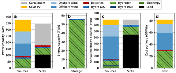
Figure 1. Cost-optimal system configuration. (a) Cost-optimal power capacity of electricity sources, that is, generators and storage charging, as well as electricity sinks, that is, storage charging. Peak load and peak curtailment is also displayed for perspective. (b) Cost-optimal storage energy capacity. (c) The 35 years average annual electricity balance. (d) Breakdown of generation and storage cost. Note that hydrogen refers to combined cycle hydrogen turbines (source), hydrogen electrolyzers (sink), as well as salt caverns (storage), and all these components are included in the hydrogen cost. Within the hydro power technologies, ROR refers to run-of-river and DIS to the dispatchable hydro reservoirs and pumped hydro storage. All storage technologies are highlighted with hatching.
Download figure:
Standard image High-resolution imageThe storage energy capacity, which is the focus of the present paper, is 56 TWh (figure 1(b)). Most of this is hydrogen storage (54.8 TWh), while existing pumped hydro storage contributes 1.3 TWh and batteries just 59 GWh (0.059 TWh). Accounting for discharging efficiency, the storage volume translates into a maximum supply of 36 TWh electricity 4 . This is about 7% of the annual load or 24 d of average load—much longer than what previous time series analyses find based on their definition of a Dunkelflaute. The storage duration is 23 d for hydrogen, 6 d for pumped hydro, and 6 h for batteries 5 .
The total primary supply from renewable sources is about 700 TWh, which is roughly 130% of the modeled annual load (figure 1(c)). The largest contribution comes from offshore wind (53%), onshore wind (26%), and solar PV (13%). Given the similar installed capacity of these variable renewable technologies, differences in energy supply are due to the diverging average capacity factors of the assumed generation profiles (0.43 for offshore wind, 0.22 for onshore wind, 0.11 for solar PV). Only 65% of the primary energy supply directly serve load (455 TWh), while 23% are charged into storage (160 TWh) and 12% are curtailed (84 TWh). Storage discharge accounts for 92 TWh (17% of load).
Although not in the focus, figure 1(d) reports the cost for storage (about €30 MWh−1 of load) and variable renewables (€50 MWh−1 of load). Note that these costs include neither the cost of existing hydro and bioenergy, nor grid cost. Nevertheless, even the approximately €80 MWh−1 of load are relatively high compared to previous studies. For example, Tröndle et al (2020) report total system costs of €50–60 MWh−1, depending on the distribution of renewables. On the one hand, the fact that we model Germany as an island may lead to an overestimation of cost. On the other hand, as opposed to previous studies, we consider multiple years of data, which means that our estimate includes the cost related to the inter-annual variability of renewables (see section 3.5).
3.2. Maximum energy deficit based on time series analysis
In this section, we analyze renewable and load times series to find the maximum energy deficit. Recall that time series of load, hydropower, and bioenergy are directly retrieved from the ENTSO-E dataset (section 2.1). For wind and solar energy, the ENTSO-E capacity factors are multiplied with the installed capacities resulting from the cost optimization model.
Because previous time series analyses identified scarcity events with a duration of up to 10 d (table A1), we first focus on the scarcest 10 d period. We find that this period occurs in December 2007. The energy deficit over this period is 12.4 TWh (8 d of average load), which is only one third of the 36 TWh of electricity that the cost-optimal storage can supply. Figure 2 displays the hourly electricity balance, including electricity generation, storage charging and discharging, load, and curtailment 6 . The figure reveals that there is very low supply from all renewable sources throughout this identified 10 d scarcity period, which is in line with the intuition behind the concept of Dunkelflaute. However, it can be seen from figure 2 that the 2 d before and the first day after the worst 10 d period are also short on energy, even though supply is not as scarce as during the 10 d. As a result, storage requirements can be expected to be defined by a period longer than 10 d. In early and late December, there is an oversupply of electricity, part of which is used to charge the hydrogen storage, while the remaining oversupply is curtailed.
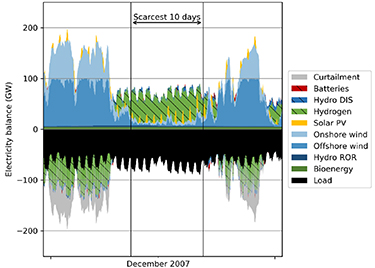
Figure 2. Hourly electricity balance for the maximum 10 d energy deficit. Electricity supply from generation and storage discharging is displayed as a stacked area with a positive sign, while electricity demand for final consumption and storage charging as well as curtailment are displayed as a stacked area with a negative sign. Storage technologies are highlighted with hatching.
Download figure:
Standard image High-resolution imageThis expectation is confirmed in figure 3(a), which displays the maximum energy deficit as a function of duration. In fact, the maximum energy deficit increases monotonically with duration for up to 14 d and starts oscillating for longer durations. Intuitively, this means that, for every increase in duration up to 14 d, another day with renewable scarcity is included in the calculation of the energy deficit; for longer durations, the period with the maximum energy deficit may also include single days with energy surplus. Furthermore, it should be noted that scarcity periods of different duration do not necessarily overlap (figure 3(b)). The scarcest periods with a duration of more than 15 d do not occur in December 2007 anymore but in November 1998; going beyond a duration of 28 d, the scarcest periods occur mostly during winter 1996–1997.

Figure 3. Characteristics of scarcity periods as a function of the considered duration  . (a) The maximum energy deficit as defined by equation (1), and (b) the corresponding start of the period
  .
.
Download figure:
Standard image High-resolution imageThe overall maximum energy deficit is 27 TWh (18 d of average load) and accumulates over 61 d (almost 9 weeks). Rather than one period with constantly low supply, these 61 d include several scarce periods in a row, interrupted by short periods with energy surplus (figure 4). This finding will be compared to the results from the cost optimization in the following.

Figure 4. Hourly electricity balance for the maximum 61 d energy deficit (the overall maximum in the 35 years dataset). Electricity supply from generation and storage discharging is displayed as a stacked area with a positive sign, while electricity demand for final consumption and storage charging as well as curtailment are displayed as a stacked area with a negative sign. Storage technologies are highlighted with hatching.
Download figure:
Standard image High-resolution image3.3. Bridging the gap between cost optimization and time series analysis
The electricity-equivalent storage energy capacity in the cost optimization model (36 TWh) is considerably higher than the maximum energy deficit identified in the time series analysis (27 TWh). This may be for two reasons. First, the cost optimization model considers storage losses, which means that one unit of excess electricity during the worst period reduces the storage requirement only by one unit of energy times the storage cycle efficiency (50.4% for hydrogen, accounting for the efficiencies of both the electrolyzer and the CCGT). By contrast, the time series analysis ignores storage losses, as one unit of excess energy reduces the energy deficit by exactly one unit. Second, the cost optimization model accounts for curtailment when excess electricity exceeds the storage charging capacity. As it can be seen in figure 4, such curtailment occurs even during the worst 61 d period. This means that it is cost-optimal to build less electrolyzers than needed to absorb all surplus electricity during the worst 61 d period and instead build a somewhat larger underground hydrogen storage to compensate for the not-absorbed surplus during the scarcity period with a higher storage level at the start of the period.
To test these potential reasons, we conduct two sensitivity runs with the cost optimization model, fixing renewable capacities. One run ignores storage losses ('no losses') and the other ignores both storage losses and charging capacity limitations ('unlimited charging'). Figure 5 reports the resulting storage volumes. As expected, both assumptions reduce storage requirements, and the results in the 'unlimited charging' scenario coincide with the maximum energy deficit calculated in the time series analysis. Put differently, to derive realistic storage requirements from time series analyses, one needs to consider charging limitations and storage losses 7 .

Figure 5. Energy storage requirements resulting from the optimization model in the reference scenario and for the hypothetical cases of loss-free storage and, in addition to the no-loss assumption, unlimited charging capacity. Note that the renewable generation capacity has been fixed for these sensitivity runs. For perspective, the figure also displays the electricity equivalent of the storage requirements in the reference scenario, that is, the aggregated maximum dischargeable electricity from all storage types.
Download figure:
Standard image High-resolution imageFinally, we identify the periods when the overall storage volume is fully used in the optimization model, that is, periods starting when all types of storage are fully charged and ending when the state-of-charge initially reaches zero. These periods define the storage requirements in the optimization model. In the sensitivity runs without storage losses, with and without charging limitations, the identified periods perfectly coincide with the worst 61 d identified with the time series analysis. Accounting for both storage losses and charging limitations, however, prolongs the worst period from 61 to 84 d (12 weeks, almost 3 months). Figure 6 reveals that this period includes the 61 d identified with the time series analysis but also about 3 weeks before this period. Accounting for charging limitations (in addition to storage losses) does not lead to a further prolongation of the worst period.
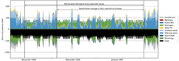
Figure 6. Hourly electricity balance for the period when storage is fully used. Electricity supply from generation and storage discharging is displayed as a stacked area with a positive sign, while electricity demand for final consumption and storage charging as well as curtailment are displayed as a stacked area with a negative sign. Storage technologies are highlighted with hatching.
Download figure:
Standard image High-resolution image3.4. Flexibility as a substitute for storage: the example of bioenergy
To enhance the comparability of the cost optimization and the time series analysis, we have so far assumed that bioenergy runs as baseload. In fact, German bioenergy-based electricity generation historically runs almost baseload at around 4.6 GW despite a much higher installed capacity of 8 GW. However, this is mostly due to inadequate regulatory incentives and market price signals and can be expected to change in a future 100% renewable electricity system (Thrän et al
2015). Against this background, we now relax this assumption, allowing for bioenergy to reduce and increase its output by ±100% (4.6 GW). As a sensitivity, we increase the maximum amount of bioenergy that can be shifted in steps of 2 TWh up to 10 TWh in electricity terms. For comparison, the assumed annual electricity production from bioenergy is 40 TWh. This means that 3 months of production can be stored, which is longer than the previously identified period when storage was fully used. The flexibility is modeled as perfect storage without losses (see appendix
The impact of flexible bioenergy on the need for other storage technologies is ambiguous. First, the electricity-equivalent volume of other storage decreases less than proportionately with increasing bioenergy flexibility (figure 7(a)). These somewhat counter-intuitive results can be explained by the fact that flexible bioenergy not only substitutes for storage but also for part of the renewable overcapacity (figure 7(d)). Second, the decrease in discharging capacity 8 equals almost exactly the capacity by which flexible bioenergy can increase production (figure 7(b)). This is intuitive to understand given that the discharging capacity must be sufficient to serve the highest residual load, which is hardly affected by the observed change in renewable capacity. Finally, when introducing bioenergy flexibility, the charging capacity initially decreases by much more than the capacity by which flexible bioenergy can decrease production (figure 7(c)). This makes sense given the reduced renewable capacity and, therefore, less renewable surplus. When further increasing the amount of shiftable electricity generation from bioenergy, however, the storage charging capacity re-increases, mostly due to additional hydrogen electrolyzers. To understand this result, it is worth highlighting that we are increasing the bioenergy flexibility only in energy terms, not in power terms. Apparently, complementing this increase in energy-related flexibility of bioenergy with an increase in power-related flexibility of hydrogen storage is a cost-efficient solution, enabling a further reduction in renewable capacity. Interestingly, the decrease in renewable overcapacity in parallel to the increase in overall storage volume means that the period when storage is fully used, that is, the period that defines storage requirements, is prolonged to more than 1 year (10 October 1995 to 3 February 1997). Hence, given the additional flexibility of bioenergy, storage requirements are defined by the inter-annual variability of renewables rather than more short-term extreme events.

Figure 7. The implications of bioenergy flexibility, assuming a varying amount of shiftable electricity (x-axis) and a maximum power adjustment of ±4.6 GW compared to the constant 4.6 GW profile in the reference scenario. The figure displays the results of the cost optimization model for (a) energy storage requirements, including the assumed flexibility of bioenergy, both displayed in terms of electricity, (b) storage discharging capacity including the assumed 4.6 GW upward flexibility of bioenergy, (c) storage charging capacity including the assumed 4.6 downward flexibility of bioenergy, and (d) the renewable generation capacity.
Download figure:
Standard image High-resolution image3.5. Comparing multi- and single-year optimization
This section contrasts the results from the multi-year optimization to those based on single years. In the multi-year optimization, we found that storage requirements are defined by a winter period crossing the turn of the calendar year. To capture this period in one of the single-year optimizations, we now consider 12 months periods from July to June of the next year instead of calendar years. For comparability, bioenergy is assumed to be inflexible again.
Figure 8 presents the distribution of the single-year results relative to the multi-year results. The investment in variable renewables varies significantly (figure 8(a)). This may be linked to the inter-annual variability of renewable energy sources, but the link is not straightforward. Relatively high and steady energy yields of a renewable technology for 1 year may reduce this technology's capacity need to supply a given share of load. However, high and steady yields may also increase the economic attractiveness of this renewable technology relative to other technologies, such that its share in electricity supply may increase. Apparently, this trade-off is solved in the single-year optimizations with a tendency toward more solar and less wind power in single-year optimizations. There is also a tendency toward more batteries (figures 8(b)–(d)), which is correlated with solar deployment. For hydrogen storage, which is decisive to bridge the largest energy deficit, the relative variation is less pronounced, but it should be noted that the absolute hydrogen storage volume is in the TWh scale while batteries are deployed in the GWh scale. As a result, hydrogen storage requirements almost directly translate to overall storage requirements (recall figure 1(b)). Remarkably, the single-year optimization systematically underestimates long-term storage requirements: the average single-year hydrogen storage volume is only half of what is needed in the multi-year optimization. The one single year that almost matches the multi-year storage requirements is the 12 months period from July 1996 to June 1997—which includes the previously identified scarcest period. The fact that the required storage volume does not match exactly can be explained by a slightly different mix of renewables when this 12 months period is optimized in isolation. The single-year optimization also tends to underestimate cost, with 1996–1997 being closest to the multi-year estimate (figure 8(d)) 9 .

Figure 8. Single-year results divided by the results from multi-year optimization. The black lines in the middle of the boxes indicate the median, the boxes extend from the first to the third quartile (inter-quartile range), and the whiskers include the 5%–95% confidence interval of the observations. Observations outside of this confidence interval are depicted as black dots, and the white points represent the mean of the distribution.
Download figure:
Standard image High-resolution image
4. Discussion
The results of this study can be compared to the literature. First, our results based on 35 years of data support the finding from previous time series analyses that the Dunkelflaute—a period with constantly high load and low renewables—does not exceed 2 weeks (table A1). However, we demonstrate for the example of Germany that storage requirements are defined by a much longer period of about 12 weeks, including multiple periods with low renewable supply but also some surplus. With increased flexibility from bioenergy, the defining period may even be longer.
Second, our finding that single-year optimization generally underestimates the required storage volume when compared to multi-year optimization is in line with Dowling et al (2020). However, while we find that the multi-year storage need is almost equal to that of the worst single year, that study reports that multi-year storage is even larger than that. This may be explained by the larger geographical scope analyzed by Dowling et al (2020) compared to the present study. Like the above-discussed effect of bioenergy flexibility, geographical smoothing may reduce variability on shorter time scales such that the remaining variability, which needs to be addressed by long-term storage, spans multiple years. Note that both single- and multi-year results on storage energy capacity lie within the wide range of results from previous cost-optimization studies (table A2).
Some limitations of the present study and possibilities for further research may be highlighted. First, for simplicity and comparability this study narrowly focuses on Germany, ignoring both international trade and intra-national grid constraints. While geographical smoothing within Europe will certainly reduce challenges and costs related to wind and solar variability, the effect on optimal storage deployment is not trivial due to the trade-off with renewable overcapacity. In this regard, it should be mentioned that during the period of the largest energy deficit in Germany—winter 1996–1997—neighboring countries were suffering severe deficits as well. This included the Swedish and Norwegian hydroelectric system, which usually exports electricity to central Europe but experienced its historically highest energy deficit during 1996. It is therefore unlikely that including modeling of international electricity trade would fundamentally impact our general results on storage requirements in 100% renewable electricity systems. Finally, sub-national grid constraints within countries may increase the requirement for storage and/or renewable overcapacity.
Furthermore, this study has a limited view on changes on the demand side of the electricity system. The decarbonization of other energy sectors may require additional electricity for electric heat pumps, electric vehicles, and the production of synthetic fuels (Ruhnau et al 2019). Our input load time series already consider part of this for the horizon of 2030, but a fully decarbonized system is likely to require a further increase in electricity demand and hence larger storage volumes. However, this demand increase will come with changes in the demand profile and the related flexibility, and further research will be needed to characterize the impact on storage requirements. Furthermore, we ignore load shedding, which may substitute for part of the storage requirements.
Finally, future load and renewable profiles may change due to climate change, which has been neglected in the current analysis. While the impact of climate change on wind and solar output is subject to large uncertainty (Bloomfield 2021), extreme events are likely to increase (Bennett et al 2021). Hence, storage requirements may be even higher than our estimates. Furthermore, it should be noted that, even without climate change, our analysis is limited to 35 years of historical data and more extreme events may occur within a longer time span (e.g. once in 100 years).
Despite these limitations, our quantitative results on storage requirements may be compared with the size of existing energy storage. The estimated 59 GWh of required battery storage in our reference scenario mean a 40-fold increases versus the 1.5 GWh installed capacity of small- and large-scale batteries in Germany 2018 (Figgener et al 2020). While a 40-fold increase in stationary battery storage may seem a lot, it is relatively little when compared to the battery requirements of passenger car electrification: equipping the about 40 million cars in Germany with 50 kWh of battery storage each would make up for 2 TWh of total battery storage capacity.
For underground hydrogen storage, current installations in Germany are limited to pilot systems. As an alternative, the currently 250 TWh of German natural gas storage, which is mostly underground storage in salt caverns, may serve as a (Sterner et al 2015). After accounting for the 70% lower volumetric energy density of hydrogen and an about 20% lower feasible peak pressure 10 , this is in the same order of magnitude as the estimated 56 TWh of required hydrogen storage in our reference scenario. Furthermore, a recent study suggests that the technical potential for underground hydrogen storage in Germany is 9.4 PWh, which is two orders of magnitude larger than our identified storage requirements (Caglayan et al 2020).
5. Conclusions
This study analyses storage requirements in a 100% renewable electricity system for the example of Germany, using 35 years of hourly time series data for renewable generation and load. With a cost optimization model, we find that the optimal storage size is 56 TWh for an assumed annual electricity demand of 540 TWh. The storage is primarily hydrogen in salt caverns (54 TWh) and large enough to supply 24 d of average load (36 TWh electricity). If one assumes a larger annual future demand, as it appears likely fully decarbonized German energy system, the relative values (i.e. days of average load) may be used as a rough guidance. Our time series analysis reveals that the maximum energy deficit occurs over a period of 9 weeks, which is much longer than the previously identified 2 weeks of consistently low supply. In fact, this longer storage defining periods consists of multiple scarcity periods, which closely follow each other. When considering storage losses and charging limitations for the surplus in between these scarcity periods, the period defining storage requirements extends over as much as 12 weeks. Using the example of bioenergy, we find that adding other sources of flexibility substitutes for storage requirements and renewable overcapacity, and the duration of period that defines storage requirements lengthens to more than 1 year. Our interpretation of this result is that the role of storage transitions from bridging extreme events toward smoothening out the inter-annual variability of wind and solar energy. Finally, when optimizing system costs based on single years rather than multi-year time series, we find substantial inter-annual variation in the overall storage requirements with the average year needing less than half as much storage as calculated for all 35 years together.
Based on our results, we conclude that focusing on short extreme events or single years can be misleading when estimating the amount of storage needed in 100% renewable electricity systems. Instead, for the example of Germany, storage requirements are defined by a 12 weeks or longer period of intermittent scarcity, and system planning based on average years significantly underestimates storage requirements and system costs. Despite these economic challenges and remaining technological uncertainty with a large-scale deployment of hydrogen infrastructure, the estimated necessary storage energy capacity seems feasible when compared to the current German natural gas storage capacity.
Acknowledgments
We gratefully acknowledge funding by the Rodel Foundation. Furthermore, we thank Georg Thomaßen, Martin Kittel, and the participants in the Hertie School's Energy Research Seminar for valuable comments and interesting discussions.
Data availability statement
The programming code of the cost optimization model is available at https://github.com/oruhnau/re100.
No new data were created or analyzed in this study.
Appendix A.: Tabular literature review
Table A1. Previous studies on low-wind events.
| Cannon et al (2015) | Patlakas et al (2017) | Ohlendorf and Schill (2020) | |
|---|---|---|---|
| Definition | Capacity factor below 10% | Wind speed below 3 m s−1 | Mean capacity factor below 10% |
| Regional scope | Great Britain | North Sea | Germany |
| Temporal scope | 33 years | 10 years | 40 years |
| Maximum duration | <4 d | Near shore: 10 d Open sea: 4–5 d | 10 d |
Table A2. Storage requirements in cost optimization studies.
| Region | Optimization period | Maximum storage discharge per average load a | |
|---|---|---|---|
| Bussar et al (2014) | Europe | 3 years | 15 d |
| Schill and Zerrahn (2018) | Germany | 1 year | 12 d |
| Child et al (2019) | Europe | 1 year | 32 d |
| Tröndle et al (2020) | Europe | 1 year | 12 d |
| Neumann and Brown (2021) | Europe | 1 year | 23 d |
Appendix B.: Detailed description of the cost optimization model description
This appendix describes the equation system of the cost optimization model. For the multi-year optimization, the model covers the entire 35 years time span with an hourly resolution with  . Decision variables are written in capitals, and parameters are lowercased.
The optimization model minimizes total system cost:
where  are the generation and discharging capacities of all investable generation and storage technologies
 , with the corresponding annualized fixed costs
  . Analogously,
  and
and  are the charging and energy capacities of the investable energy storage technologies
  ,
,  and
and  are the corresponding annualized fixed costs. Because battery inverters can be used for both charging and discharging, investment cost are only considered for discharging and
  . The sum of the hourly curtailment
  is subtracted from the cost function with a very small coefficient
  to ensure that electricity is rather curtailed than stored and, thereby, avoid arbitrary solutions regarding storage utilization.
The main constraint of the model is the electricity balance:
where  is the load time series from ENTSO-E.
  is the hourly generation from the investable renewable technologies
  , and
, and  is the generation from the exogenously fixed renewable technologies
  .
.  and
and  are the hourly discharging and charging variables of the storage technologies
  .
.
A capacity constraint relates the hourly generation of the investable renewable technologies to the corresponding capacity variable:
where  are the hourly renewable capacity factors from ENTSO-E.
Finally, the model includes the following five storage constraints:


The first of these constraints equation (B4) relates the storage level in 1 h to the level in the preceding hour, considering storage charging, discharging, and the hourly natural inflow of the dispatchable hydropower plants  according to ENTSO-E (for the other storage technologies, the inflow parameter is zero). The constraints equations (B5)–(B7) ensure that the maximum discharging, charging, and energy capacity of storage is respected. For the hydro DIS, the capacity variables are fixed to the existing capacity.
For the sensitivity with flexible bioenergy, a new storage technology  is introduced with charging and discharging capacities fixed to 4.6 GW, and the exogenously defined storage energy capacity varying from 0 to 10 TWh. The storage charging and discharging efficiencies are set to unity to reflect our assumption that electricity generation from bioenergy can be shifted without affecting the overall generation.
The model was implemented in the modeling software GAMS and needs less than 2 h to solve on an individual computer using the solver CPLEX.
Appendix C.: Assumptions used for the cost optimization
The cost assumptions are summarized in table C1. They are based on the 2050 estimates in de Vita et al (2018), except for the assumptions on hydrogen storage and electrolyzers, which we take from specifically hydrogen-related studies. More precisely, information on the cost of hydrogen storage in salt caverns is retrieved from the 'hydrogen supply chain evidence base' by element energy (Walker et al 2018), and the cost of electrolyzer are the average of a recent literature review (Ruhnau 2022). A discount rate of 6% is applied to the investment cost.
Table C1. Cost assumptions.
| Technology | Unit | Investment cost (unit) | Lifetime (years) | Fixed O&M a (unit p.a.) |
|---|---|---|---|---|
| Solar PV | € kW−1 | 450 | 25 | 10 |
| Onshore wind | € kW−1 | 900 | 25 | 13 |
| Offshore wind | € kW−1 | 1800 | 25 | 26 |
| Hydrogen CCGT | € kW−1 | 750 | 25 | 15 |
| Hydrogen electrolyzer | € kW−1 | 450 | 25 | 9 |
| Hydrogen storage | € kWh−1 | 2 | 25 | — |
| Battery inverter | € kW−1 | 100 | 15 | — |
| Battery pack | € kWh−1 | 125 | 15 | — |
The natural inflow to the hydro DIS is set to the sum of the weekly timeseries of natural inflow to reservoirs and to pumped hydro storage. The reservoir size is set to the sum of reservoirs (0.26 TWh) and pumped hydro (1.02 TWh), and the aggregated turbine and pump capacities are set to 8.85 and 7.96 GW, respectively. Bioenergy is assumed to constantly produce 4.6 GW, which is the average value of 2016–2020.
The cycle efficiency for pumped hydro storage and batteries is assumed to be 80% and 90%, respectively (www.eesi.org/papers/view/energy-storage-2019). The conversion efficiency of hydrogen electrolyzers and combined cycle turbines is set to 80% 11 (IEA 2019) and 63% (de Vita et al 2018), respectively. As a constraint, the storage levels at the end of 1 year must be equal to the levels at the beginning of the next year, and the storage levels at the end of the last year must be equal to the levels at the beginning of the first year. This ensures that, over the entire time span, storage charging equals storage discharging plus losses without fixing the start and end levels to arbitrary values. To avoid arbitrary results related to unintended storage cycling, a penalty term in the objective function ensures that electricity is only stored when needed and curtailed otherwise (Kittel and Schill 2021, Parzen et al 2021).
Footnotes
- 3
We mean storage volumes in terms of days of average load, which we use to make the cost optimization results comparable across different regional scopes and to the duration of the scarcity periods identified in the time series analyses.
- 4
34.5 TWh from hydrogen, 1.1 TWh from hydro power, and 56 GWh from electricity.
- 5
Here, we define this as the storage volume in electricity terms divided by storage discharge capacity (also referred to as energy-to-power ratio).
- 6
- 7
- 8
The overall decrease is mostly a reduction in combined cycle hydrogen turbines and to a lesser extend a reduction in battery power capacity.
- 9
Note that the key result that single-year optimization underestimates storage volume and cost holds true also for calendar years, but the worst single year is then different from the worst period in the multi-year optimization.
- 10
250 TWh × (1%–30%) × (1%–20%) = 57.6 TWh.
- 11
Although not unrealistic, we recognize that this value is in the upper range of what can be expected in 2050. We therefore conducted a sensitivity run with an electrolyzer efficiency of 75%, which leads to very similar results: the capacity of hydrogen salt caverns and CCGT decreases slightly by 1 TWh (2%) and 0.5 GW (1%), respectively, while the capacity of hydrogen electrolyzers increases by 1.7 GW (3%). Battery storage partly compensates for the less effective hydrogen storage with an increase in power and energy capacities by 4% and 8%, respectively. The renewable mix shifts slightly from solar PV (−2%) to wind offshore (+3%). The total cost increase by less than 1%. The storage-defining period is still 84 d long.