

Abstract
Non-perennial streams are widespread, critical to ecosystems and society, and the subject of ongoing policy debate. Prior large-scale research on stream intermittency has been based on long-term averages, generally using annually aggregated data to characterize a highly variable process. As a result, it is not well understood if, how, or why the hydrology of non-perennial streams is changing. Here, we investigate trends and drivers of three intermittency signatures that describe the duration, timing, and dry-down period of stream intermittency across the continental United States (CONUS). Half of gages exhibited a significant trend through time in at least one of the three intermittency signatures, and changes in no-flow duration were most pervasive (41% of gages). Changes in intermittency were substantial for many streams, and 7% of gages exhibited changes in annual no-flow duration exceeding 100 days during the study period. Distinct regional patterns of change were evident, with widespread drying in southern CONUS and wetting in northern CONUS. These patterns are correlated with changes in aridity, though drivers of spatiotemporal variability were diverse across the three intermittency signatures. While the no-flow timing and duration were strongly related to climate, dry-down period was most strongly related to watershed land use and physiography. Our results indicate that non-perennial conditions are increasing in prevalence over much of CONUS and binary classifications of 'perennial' and 'non-perennial' are not an accurate reflection of this change. Water management and policy should reflect the changing nature and diverse drivers of changing intermittency both today and in the future.
Export citation and abstract BibTeX RIS
1. Introduction
Non-perennial streams—referring to streams and rivers that do not flow continuously, including intermittent rivers and ephemeral streams (Busch et al 2020)—are present across all global continents, ecoregions, and climate types (Messager et al 2021) and provide many ecosystem services such as agricultural and domestic water supply while sustaining the ecological integrity of river networks (Datry et al 2018a, Kaletová et al 2019, Stubbington et al 2020). Though non-perennial streams constitute over half the global stream network length (Messager et al 2021), hydrological and ecological research have predominantly focused on perennial waters, in part because gauge networks are biased toward larger rivers (Zimmer et al 2020). However, non-perennial streams have garnered increasing attention in recent years (e.g. Leigh et al 2016, Allen et al 2020, Shanafield et al 2020, 2021).
Recent efforts have quantified spatial patterns of stream intermittency at regional (Datry et al 2016, Allen et al 2019, Jaeger et al 2019), national (Snelder and Booker 2013, Beaufort et al 2018, Hammond et al 2021, Sauquet et al 2021), and global (Messager et al 2021) scales. These studies provide a useful framework for classifying and understanding spatial patterns in stream intermittency during a particular study period. However, temporal changes in stream intermittency are inadequately studied, despite documented widespread change in the perennial flow regime including low flows (Ficklin et al 2018, McCabe and Wolock 2002, Dudley et al 2020, Rodgers et al 2020). Given the strong influence of stream intermittency on aquatic biodiversity (Jaeger et al 2014, Datry et al 2014b) and water quality (Datry et al 2018b, Gómez-Gener et al 2020), a pressing question thus remains: is stream intermittency changing at regional to continental scales, and if so, what are the characteristics and causes of this hydrologic change?
Non-perennial streams are rarely considered in water management (Acuña et al 2014) despite their widespread nature and the numerous ecosystem services they provide. Open questions about the locations, functions, and connectivity of non-perennial streams to downstream waters have become a central focus of U.S. litigation and agency rulemaking to clarify a basis for protecting these ecologically important headwaters (Walsh and Ward 2019) as they can be disproportionately important to downstream water quality (Dodds and Oakes 2008). Thus, improved understanding of both current non-perennial flow regimes, as well as how they are changing, is critical to proactive and effective management (Sills et al 2018, Sullivan et al 2020). Potential increases in stream intermittency deeply affect our ability to meet both agricultural and domestic water requirements, especially in arid regions (Cudennec et al 2007). As such, understanding the large-scale trends and drivers of change in stream intermittency is a critical need to anticipate management priorities, guide water policy, and sustain both ecosystems and society.
We investigated the trends and drivers of change in non-perennial streamflow across the continental United States (CONUS) to meet these critical needs. Specifically, we asked: (1) How have different aspects of stream intermittency changed through time across CONUS?, and (2) What are the drivers of spatiotemporal variability in stream intermittency? We answered these questions using all 540 non-perennial U.S. Geological Survey gages in CONUS with at least 30 years of daily streamflow data within the period 1980–2017. We used these data to explore trends and the magnitude of change for three intermittency signatures: the number of no-flow days per year (a signature for no-flow duration), the number of days from peak flow to no-flow (a signature for dry-down period), and the date of the first no-flow observation (a signature for no-flow timing). We also developed random forest models to identify the watershed climate, land/water use, and physiographic characteristics that best predicted spatiotemporal variability for each of these intermittency signatures to identify potential drivers of change. Finally, we summarized the societal and environmental importance of these ongoing changes to stream intermittency.
2. Methods
2.1. Gage selection
Our data incorporated 540 gages (figure 1) from the US Geological Survey (USGS) GAGES-II dataset, which encompasses 9322 stream gages that have at least 20 years of data and/or are currently active (Falcone 2011). Since the focus of our analysis was trends in non-perennial streams, we selected all streams with at least 30 years of data between the 1980 and 2017 climate years (April 1–March 31) and had an average no-flow fraction of at least 1.4% (corresponding to 5 d year−1) but no greater than 98.6% (corresponding to 360 d year−1). These criteria retained a sample of 540 gages, in watersheds ranging from 0.95 to 49 264 km2 (figure S1, available online at stacks.iop.org/ERL/16/084033/mmedia). We grouped gages into six ecoregions based on modified US Environmental Protection Agency level 1 ecoregions: (1) Eastern Forests (n = 136 gages), (2) Mediterranean California (n = 87 gages), (3) North Great Plains (n = 56 gages), (4) South Great Plains (n = 157 gages), (5) Western Deserts (n = 40 gages), and (6) Western Mountains (n = 64 gages). More details on regions are found in supplemental information (section SI1).

Figure 1. Map of USGS gages used in analysis, colored by region.
Download figure:
Standard image High-resolution image2.2. Intermittency signatures
Hydrologic signatures are metrics extracted from hydrographs that isolate particular types of hydrological processes (Olden and Poff 2003, McMillan 2020). We focused on three hydrologic signatures (referred to as 'intermittency signatures') that describe: (1) the annual no-flow duration, calculated as the number of days with zero discharge per year; (2) the dry-down period, calculated as the number of days from a local peak (exceeding 25th percentile of long-term mean daily flow) to a zero discharge measurement; and (3) the no-flow timing conditions, calculated as the first day of the climate year at which a zero discharge measurement occurred. Each intermittency signature was calculated on an annual basis from raw streamflow data rounded to one decimal place in order to reduce noise in low-flow conditions. For the dry-down period, the days from peak to no-flow were calculated for each no-flow event, and averaged to an annual value based on the climate year of the no-flow date.
2.3. Change analysis
We used the non-parametric Mann-Kendall trend test to estimate the trend in each intermittency signature and climate metric at each gage. Mann-Kendall tests were only calculated where there are at least 10 years of data, which included 540 gages (the entire sample) for the climate metrics and annual no-flow days, but was only possible with 473 gages (87.6%) for the days from peak to no-flow signature and 475 gages (88%) for the day of first no-flow. These two intermittency signatures have fewer data points than annual no-flow days because they can only be calculated in years where flow ceases. Since the Mann–Kendall test only provides information about the trend, but not the magnitude of change, we complemented the Mann–Kendall test with a Mann–Whitney test, in which data for each gage were split into two halves (1980–1998 and 1999–2017; figure S6). We also tested the sensitivity of Mann-Whitney results to the split year (section SI2.4). The Mann–Whitney test evaluates the probability of the mean of one group being higher than the mean of the other. Mann–Whitney tests were only calculated where there are at least 10 total years of data and at least 5 years of data within each group. Like the Mann–Kendall tests, this included all gages (n = 540) for the climate metrics and annual no-flow days, but fewer gages for peak to no-flow (n = 425) and the day of first no-flow (n = 428). For both Mann–Kendall and Mann–Whitney tests, we used a significance level of p < 0.05. Some gages exhibited very large, non-linear changes within the study period (figure S3), justifying our use of the Mann–Kendall and Mann–Whitney approaches to characterize trends and magnitudes of change rather than a simple linear or Sen's slope.
2.4. Drivers analysis
We developed random forest models (Breiman 2001) to quantify drivers of change by predicting each intermittency signature as a function of climate, land/water use, and physiographic properties of the watershed. Random forest models, a type of non-parametric machine learning approach, are well-suited for hydrological prediction due to their ability to handle numerous predictors with potentially nonlinear and interacting relationships, relatively low risk of overfitting to an anomalous subset of the sample data, and ease in interpreting the importance of each input variable (Eng et al 2017, Addor et al 2018, Miller et al 2018). We developed a total of 21 separate random forest models, based on a combination of the three intermittency signatures and seven regions (i.e. a national model including all gages, and a regional model for each of the six regions shown in figure 1). For each random forest model, we followed the same approach, which is described in detail in Section SI3. In brief, we used an 80% training and 20% testing data split, stratified by region and whether a gage was classified as reference or non-reference in the GAGES-II dataset. For each intermittency signature, there were a total of 85 candidate predictor variables, representing climate, land/water use, and physiographic characteristics (table 1). We used a systematic approach to eliminate candidate predictor variables with near-zero variance and highly correlated variables (r > 0.9), leaving a set of 56 candidate predictor variables, which are noted in the 'Retained after predictor screening' column of table 1.
Table 1. Predictor variables used in random forest models, including the source with development, validation, and/or QA/QC information.
| Name | Description [units] | Retained after predictor screening | Source and availability |
|---|---|---|---|
| Climate variables (n = 60). Annual and seasonal (AMJ, JAS, OND, JFM) values for current climate year (CY) and prior climate year (CY-1) for each variable | |||
| P | Total precipitation [mm] | CY-1: AMJ, JAS, OND, JFM CY: OND, JFM | gridMET (Abatzoglou 2013). Available in near real time 1979–present at daily timesteps and 4 km spatial resolution |
| PET | Total ASCE grass reference evapotranspiration [mm] | CY-1: AMJ, JAS, OND CY: CY, AMJ, JAS, OND | |
| Tmax | Mean daily maximum temperature [°C] | CY-1: None CY: CY, JAS, OND, JFM | |
| P/PET | Ratio of P to PET [—] | CY-1: CY, OND, JFM CY: CY, JAS | Calculated as (P)/(PET) |
| SWE | Total snow water equivalent [mm] | CY-1: OND, JFM CY: CY, OND | NSIDC (Broxton et al 2019). Available 1981–2017 at daily timesteps and 4 km spatial resolution |
| SWE/P | SWE as a fraction of total P [—] | CY-1: CY, AMJ, OND, JFM CY: CY, AMJ, OND, JFM | Calculated as total (SWE)/(PET) for time period |
| Land/water use variables (n = 13) | |||
| Water | Water land cover [% of watershed] | Yes | Available annually 1980–1991 (Sohl 2018), 1992–2005 (Sohl et al 2018), then 2006, 2011 and 2016 through NLCD (Homer et al 2007, Fry et al 2011, Homer et al 2015). Annual time series generated by linear interpolation between years with data, with 2016 value used for 2016–2017 |
| Wetland | Wetland land cover [% of watershed] | Yes | |
| Forest | Forest land cover [% of watershed] | Yes | |
| Grass | Grassland land cover [% of watershed] | Yes | |
| Developed | Developed land cover [% of watershed] | Yes | |
| Barren | Barren land cover [% of watershed] | Yes | |
| Agriculture | Agricultural land cover [% of watershed] | Yes | |
| Irrigation | Irrigated cropland [% of watershed] | Yes | GAGES-II (Falcone 2017). Available at 10 year intervals, 1982–2012. Annual time series generated via linear interpolation between years with data, with 1982 value used for 1980–1982 and 2012 value used for 2012–2017 |
| # Dams | Dams in watershed [count] | Yes | Available in 1980, 1990, 2000, 2010, 2013 (Wieczorek et al 2018). Annual time series generated based on value for closest year |
| # Major Dams | Major dams in watershed [count] | Yes | |
| Dam Max Storage | Maximum dam storage in watershed [acre-feet] | No | |
| Dam Norm Storage | Normal dam storage in watershed [acre-feet] | No | |
| Water Use | Water use within watershed [megaliters year−1 square km−1] | Yes | USGS (Falcone 2016, Falcone 2017). Available at 5 year intervals, 1985–2010. Annual time series generated via linear interpolation between years with data, with 1985 value used for 1980–1985 and 2010 value used for 2010–2017 |
| Physiography variables (n = 12) | |||
| Drainage area | Watershed drainage area [km2] | Yes | Included in GAGES-II dataset (Falcone 2011) |
| Elevation | Mean elevation in watershed [m] | Yes | |
| Slope | Mean slope in watershed [%] | Yes | |
| Soil Permeab | Mean soil permeability in watershed [in h−1] | Yes | |
| Soil clay | Mean soil clay content [%] | Yes | |
| Soil silt | Mean soil silt content [%] | Yes | |
| Soil sand | Mean soil sand content [%] | No | |
| Soil AWC | Mean soil available water content [—] | Yes | |
| Topo wetness | Mean Topographic Wetness Index [—] | Yes | |
| Bedrock depth | Mean depth to bedrock in watershed [m] | Yes | SoilGrids (Hengl et al 2017) |
| Porosity | Mean aquifer porosity [—] | Yes | GLHyMPS (Gleeson et al 2014) |
| Storage | Mean watershed storage [m] | No | Calculated as (porosity) * (bedrock depth) |
We then constructed an initial random forest model for each intermittency signature using all 56 predictor variables retained after predictor screening (table 1) and extracted conditional variable importance for each candidate predictor variable (Strobl et al 2008), which accounts for collinearity among candidate predictor variables. This generated a ranked list of all predictor variables for each model. We then built final random models for each intermittency signature using the number of most important predictor variables that minimizes out-of-bag mean squared error (MSE). To estimate the relative importance of different predictor variables in our final model (i.e. figure 6), we used the permutation-based increase in MSE for each predictor variable, expressed as a percentage of the overall model MSE. A higher MSE increase indicates that the predictor variable has a greater influence on model predictors for the out-of-bag sample used in model training.
We calculated model fit based on the test sample that was not used for model training (table S2). We used four different statistical measures of model performance: R2; root mean squared error (RMSE); normalized RMSE, which is the RMSE divided by the range of observed values; and Kling–Gupta Efficiency (KGE), which is a performance metric that accounts for bias, correlation, and variability (Gupta et al 2009). Using regional submodels slightly improved overall model performance compared to the national models (figure S14), but the improvement was marginal, so for our results and analysis we focused on the national models to better understand large-scale variability and drivers of change across all of CONUS.
3. Results
3.1. Changing stream intermittency
Half the CONUS non-perennial gage network had a significant trend in no-flow duration, dry-down period, and/or no-flow timing over the study period (figure 2). Mann–Kendall tests indicated significant (p < 0.05) trends in the number of annual no-flow days for 41% of gages (26% longer duration, 15% shorter duration; figure 2(a)). Significant trends were less common for the dry-down period (17% of gages; figure 2(b)) and no-flow timing (15% of gages; figure 2(c)), but gages with significant trends in these signatures were primarily shifting towards drier conditions, as characterized by a shorter dry-down period (10% of gages) and an earlier onset of no-flow conditions (12% of gages).
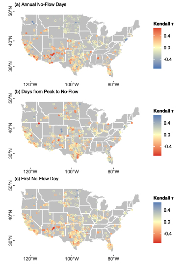
Figure 2. Mann–Kendall trends in (a) annual no-flow days, (b) days from peak to no-flow, and (c) first no-flow day. In all Mann-Kendall plots, red indicates drier conditions (longer no-flow duration, shorter dry-down period, earlier first no-flow day).
Download figure:
Standard image High-resolution imageShifts towards more intermittent flow dominated the southern half of CONUS, while decreased intermittency indicating wetter conditions was prevalent in the northern half of CONUS (figure 3). Trends for duration and timing were closely related, where a longer no-flow duration corresponded to an earlier onset of no-flow conditions (r = −0.64; figure S2). For both annual no-flow days and timing of first no-flow day, we found drying trends in the Mediterranean California, Southern Great Plains, Western Mountains, and Western Desert ecoregions and at low latitudes, while wetting trends were more common in the Northern Great Plains ecoregions and at high latitudes (figure 3). The Eastern Forests ecoregion, which spans most of the eastern half of the United States (figure 1), demonstrated both positive and negative trends for the no-flow duration and timing, but drying trends were still concentrated in the south and wetting trends in the north (figures 2 and 3). By contrast, there was less spatial coherence in trends for the dry-down period (figures 2(b) and 3(b)).

Figure 3. Mann-Kendall trends summarized as violin plots by (left) region and (right) latitude for (a) annual no-flow days, (b) days from peak to no-flow, and (c) first no-flow day, with median of distribution marked. For left column, the number along the x-axis indicates the number of gages in that sample. For latitude plots, y-axis label corresponds to the center of a 3° band.
Download figure:
Standard image High-resolution imageTo complement the trend analysis, which only reflects the direction and significance of change, we estimated the magnitude of change at each gage using the Mann–Whitney test. As with the trends analysis, we found that half the gage network had a significant change (p < 0.05) in at least one intermittency signature between the first half (1980–1998) and the second half (1999–2017) of the study period: 38% of gages had a significant change in the annual number of no-flow days (27% drier, 11% wetter), 21% of gages had a significant change in the days from peak to no-flow (12% fewer, 9% more), and 21% of gages had a significant change in no-flow timing (16% earlier, 5% later). A sensitivity analysis found that these results are robust to the choice of year used to split the data into two groups. Regardless of the year used to split the data there were widespread significant changes in the intermittency signatures, particularly the annual number of no-flow days, with drying more common than wetting (see supplemental information, section SI2). These changes exhibit a similar spatial pattern to the results of the trend analysis, with drying in the south and wetting in the north (figure 4). The magnitude of change during the period varied widely, with significant changes in no-flow duration ranging from −214 d to +262 d, and smaller ranges for the dry-down period (−57 to +145 d) and timing (−124 to +163 d) of no-flow (figures 4(a)–(c)).

Figure 4. Stacked histograms (a)–(c) and maps (d)–(f) showing Mann–Whitney change test results for (a), (d) annual no-flow days, (b), (e) days from peak to no-flow, and (c), (f) first no-flow day. Change tests compare the second half of the period of record (1999–2017) to the first half of the period of record (1980–1998), and units for all plots are days. Only gages with significant changes (p < 0.05) shown on maps. In all plots, red indicates drier conditions (longer no-flow duration, shorter dry-down period, earlier first no-flow day) and blue indicates wetter conditions.
Download figure:
Standard image High-resolution image3.2. Drivers of stream intermittency variability and change
Trends in the ratio of annual precipitation to potential evapotranspiration, P/PET (commonly known as the aridity index) were significantly correlated with trends in the annual no-flow days (r = − 0.42; p < 0.001; figure 5(a)) and the no-flow timing (r = 0.27; p < 0.001; figure 5(c)). A negative P/PET trend indicating drier climatic conditions is associated with a decrease in precipitation and/or an increase in PET. Thus, trends toward a longer duration and earlier onset of annual no-flow conditions are accompanied, and potentially caused, by drier climatic conditions. However, trends in peak to no-flow days were not associated with P/PET trends (r = 0.05; p = 0.3; figure 5(b)). The lack of a relationship suggests that climatic drying was not a notable driver of long-term change in dry-down period. Furthermore, at the regional scale, observed trends in annual no-flow days and timing (figure 3) are consistent with regional-scale trends in P/PET (figures S4 and S5), though there are regional differences in the strength of the relationship between the P/PET trend and the intermittency signature trends. In contrast to the other intermittency signatures, we found less regional coherence between aridity and changes in the dry-down period compared to no-flow timing or duration, providing additional support of the Mann-Kendall and Mann-Whitney test results (figures 3(b) and 4(e)).
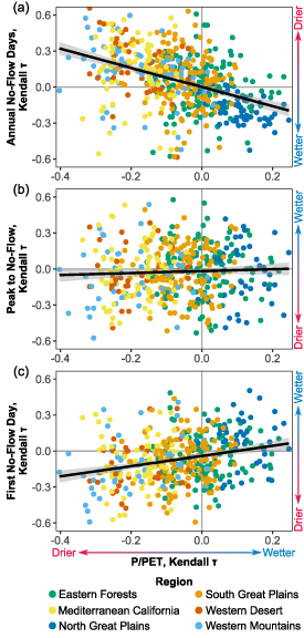
Figure 5. Comparison of Mann-Kendall trends for (a) annual no-flow days, (b) days from peak to no-flow, (c) first no-flow day, against the Mann-Kendall trend for the ratio of annual precipitation to potential evapotranspiration (P/PET). Black line shows a linear best fit with 95% confidence interval shaded. Pearson correlations are (a) r = − 0.42, (b) r = 0.05, (c) r = 0.27.
Download figure:
Standard image High-resolution imageThe importance of changes in P and PET to P/PET trends varies across regions. In the Northern Great Plains, for instance, there is a positive (drying) median PET trend but it is weaker in magnitude than the positive (wetting) median P trend, and therefore the region-wide median P/PET trend indicates wetting conditions (figure S4). A similar dynamic is present to a lesser degree for the Eastern Forests region, in which positive trends in P and PET approximately cancel out so that the median P/PET trend is 0. By contrast, the regions in the western US (Western Mountains, Western Deserts, Mediterranean California) have both negative P trends and positive PET trends, both of which contribute to an overall drying P/PET trend. Since the PET product we used is calculated using the ASCE Penman–Monteith approach (Abatzoglou 2013), increases in PET may be driven by a variety of factors including increases in the vapor pressure deficit associated with warmer temperatures, increased turbulent transport due to greater wind speed, and/or greater incoming solar radiation. Furthermore, our analysis does not measure potential changes in the timing of P and PET within the year, apart from the inclusion of seasonal indicators as part of our random forest analysis (table 1).
We used random forest regression models to further explore drivers of spatiotemporal variability in each intermittency signature. These models provided annual-resolution predictions of no-flow days, days from peak to no-flow, and the timing of the first no-flow day for each gage as a function of climate, land/water use, and physiography within the contributing watershed. Model performance, evaluated using independent test data not used for model development (see Materials and Methods section), was strong for all intermittency signatures and regions (table S2 and figure S12), with the best fit for no-flow duration (R2 = 0.77, KGE = 0.71), followed by no-flow timing (R2 = 0.52, KGE = 0.52), and dry-down period (R2 = 0.35, KGE = 0.39). These performance scores exceed typical benchmarks for identifying behavioral hydrological models (KGE > 0.3; Knoben et al 2019) indicating they are adequate tools to identify the relative influence of different watershed variables on predicted intermittency signatures.
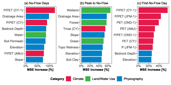
The number of annual no-flow days was sensitive to a combination of climatic and physiographic variables. The most influential predictor variable was P/PET of the preceding climate year, followed by the gage's drainage area and P/PET for the current climate year (figure 6(a)). By contrast, the dry-down period was primarily sensitive to land/water use and physiography, with wetland cover, drainage area, and forest cover as the most influential predictor variables (figure 6(b)). Predictions of the no-flow timing were highly sensitive to climate conditions from the preceding year. The most influential predictor was P/PET for the preceding climate year, followed by P/PET for the end of the preceding climate year (January, February, and March) (figure 6(c)). Notably, for both the no-flow duration and timing, preceding year climate conditions had a stronger influence on annual intermittency signatures than climate conditions in the year of interest, indicating that there are time lags between climatic drivers and stream intermittency response. These time lags suggest that climate controls on stream intermittency are moderated by watershed properties that control the storage and release of water from the landscape, which is further supported by the strong influence of physiographic variables such as drainage area, bedrock depth, soil permeability, and slope in the random forest models (figure 6). Human impacts are substantial for many of the gages in our sample. For instance, 64% of gages are downstream of at least one dam and there is at least 10% human-modified land use (agricultural or developed) in the watersheds for more than half of gages. Despite these widespread human impacts, variables associated with human modification of the water cycle (such as irrigation extent, water use, and dam storage; table 1) were not identified as highly influential predictor variables over any of the intermittency signatures.
Figure 6. Top nine predictor variables for (a) annual no-flow days, (b) days from peak to no-flow, (c) first no-flow day. For climatic variables, (−1) indicates conditions from the preceding year. The 'MSE Increase [%]' is the change in mean squared error (MSE) when that variable is randomly permuted, expressed as a percentage of overall model MSE, and a higher value is interpreted as a more important variable. Variable names are defined in table 1.
Download figure:
Standard image High-resolution image
4. Discussion
4.1. Hydrological change in context
Our study revealed widespread and primarily drying trends in stream intermittency across CONUS, indicating a temporal and potential spatial expansion of non-perennial flow regimes. Intermittency trends showed spatial coherence, with most southern gages demonstrating an increase in no-flow duration, primarily associated with increasing trends in aridity (figures 5 and 6). Aridity is a strong predictor of annual stream intermittency in regional, national, and international studies (Jaeger et al 2019, Hammond et al 2021, Messager et al 2021, Sauquet et al 2021), and here we demonstrate that changes in aridity through time are also contributing to significant and widespread changes in multiple aspects of stream intermittency. Only a subset of gages located in the Northern Great Plains (15% of gages) had trends towards fewer annual no-flow days during the period of analysis. The cold-season intermittency (Eng et al 2016), decreasing seasonal freezing, and increasing precipitation in the region (figure S4) could drive the observed reduction in no-flow conditions.
The significant changes in stream intermittency we observed during the 1980–2017 period provide a multi-decadal window into a long-term trajectory of change. Since our dataset does not include any hydrologic change that happened prior to 1980, our analysis likely underestimates long-term changes in stream intermittency relative to pre-development conditions. Irrigation expanded rapidly across much of CONUS during the 1940–1980 period (Kustu et al 2010), leading to substantial reductions in perennial stream length prior to 1980 in some regions (Perkin et al 2017). Looking forward, projected climate and land/water use change may lead to further changes in stream intermittency across much of CONUS. For instance, much of the western US and Great Plains regions are projected to experience drier climate throughout the 21st century (Ryu and Hayhoe 2017, Seager et al 2017a, 2017b, Cook et al 2020), continuing or potentially exacerbating the observed trend of increasing stream intermittency we document in these regions. Given the role of watershed storage as a buffer against climate variability, as evidenced by the importance of physiographic variables in the random forest models (figure 6), climate change-induced future shifts in stream intermittency may be most immediately felt in regions with relatively little watershed storage (i.e. smaller headwater catchments; Costigan et al 2015, Zimmer and McGlynn 2017) and/or locations with ongoing storage losses (i.e. due to pumping-induced groundwater and streamflow depletion; Perkin et al 2017, Zipper et al 2019, 2021, Compare et al 2021).
Our analysis identified significant and quantifiable predictors of no-flow at broad spatial scales. The clear regional and latitudinal patterns we identified (figure 3) contrast with continental-scale work in Europe that showed little spatial correlation in stream intermittency trends (Tramblay et al 2021). This may be due to greater regional coherence of historical P/PET trends in CONUS (figure S4) compared to Europe, where regional-scale atmospheric circulation indicators were not strongly associated with stream intermittency (Tramblay et al 2021). The regional P/PET trends appear to contribute to the regional trends we observed in the intermittency signatures (figures 5 and 6), and in particular climate seems to drive the difference in stream intermittency between the northern and southern CONUS. By contrast, human activities such as water withdrawals and dam storage have modest influences on nationwide spatiotemporal variability in the intermittency signatures studied here. The lack of significant human impacts may reflect the fact that anthropogenic disturbances can have a variety of effects that could either increase or decrease stream intermittency (Gleeson et al 2020), and these impacts may be more localized and therefore less evident as a driver of change in our nationwide analysis. Alternately, the datasets and variables we used to quantify these activities may not adequately represent their potential impact on non-perennial flow regimes. The importance of climate as a potential driver of change also corroborates previous work focused on perennial hydrological signatures. For instance, Ficklin et al (2018) found widespread climate-driven decreases in streamflow in the southern CONUS and increases in streamflow in the northern CONUS, which were primarily associated with climate change and present in both natural and human-impacted watersheds. Similarly, other work at regional to global scales has also demonstrated that climate change is the dominant forcing associated with long-term change in perennial hydrological systems, though anthropogenic water and land management also have a significant and widespread effect (Rodgers et al 2020, Gudmundsson et al 2021).
Our results provide evidence that no-flow duration, no-flow timing, and dry-down period are more predictable than indicated by previous efforts. Although others have found correlations between stream intermittency and climatic signatures such as effective precipitation or aridity at a site to regional scale (Blyth and Rodda 1973, Jaeger et al 2019, Ward et al 2020, Compare et al 2021), hydrologic signatures related to low-flow and no-flow conditions are among the most challenging to predict at continental scales (Eng et al 2017, Addor et al 2018). Our random forest models (described in detail in section SI3) compared favorably to previous studies, with a R2 of 0.77 for no-flow days (table S2) compared to an R2 of ∼0.3 for predictions of no-flow frequency from Addor et al (2018). We also found that the different intermittency signatures studied had diverse drivers, but both annual no-flow days and the timing of no-flow showed a strong dependence on antecedent (prior year) climate conditions. The importance of local factors, such as geology, soil characteristics and river network physiography (Snelder et al 2013, Costigan et al 2017, Trancoso et al 2017), indicates that some intermittency signatures (e.g. dry-down period) could be harder to predict at large scales than others (e.g. no-flow days), perhaps due to the controls of local surficial geology and perched water table dynamics on dry-down period (Costigan et al 2015, Zimmer and McGlynn 2018).
4.2. Human and environmental implications
Widespread trends towards more intermittent flow in southern CONUS have significant implications for society and water management. Non-perennial streams provide numerous ecosystem services (Datry et al 2018a, Kaletová et al 2019, Stubbington et al 2020) and shifts towards more frequent dry conditions may enhance some ecosystem services (e.g. reducing flood risk by enhancing infiltration capacity; Shanafield and Cook 2014) while decreasing others (e.g. decreasing food production and recreation through reduced fish habitat; Perkin et al 2017). By contrast, decreased cold-season intermittency in northern CONUS could lead to negative outcomes such as increased rain-on-snow driven spring flooding across the US Midwest (Li et al 2019), while improving some ecosystem services associated with water-related recreation. Effects of changing stream intermittency can also be non-local: the gages exhibiting stream intermittency we studied occurred most often in relatively small headwater catchments (figure S1), and therefore increasing stream intermittency could lead to decreases in downstream surface water availability for municipal, industrial, and agricultural needs. Ultimately, the implications of these trends for society will depend on the relative values of competing ecosystem services and the degree to which these services are replaceable (Datry et al 2018a).
The observed widespread trends in no-flow duration, dry-down period, and no-flow timing also have diverse and potentially significant implications for aquatic ecosystems, biogeochemical cycling, and water quality. These temporal and spatial trends in intermittency could inform and refine the biome-specific approach to characterizing freshwater ecosystem function (Dodds et al 2019), perhaps through the more explicit representation of the different stream drying regimes (Price et al 2021). Intermittency is a key aspect of stream 'harshness' for organisms inhabiting intermittent waters (Fritz and Dodds 2005), and we found that the duration of no-flow significantly increased at 26% of non-perennial gages indicating widespread harsher conditions for aquatic ecosystems. Stream invertebrate communities typically become less biodiverse as the duration of the no-flow period increases (Datry et al 2014a), and the annual no-flow duration is the most important hydrologic signature in explaining diversity in streams (Leigh and Datry 2017). This suggests that the widespread drying trends we found may be associated with decreasing biological diversity for most aquatic taxonomic groups. In settings where drying has historically been less common, such as humid regions, increased drying may trigger shifts to more desiccation-resistant communities (Drummond et al 2015) and therefore these settings may experience greater ecological changes in response to changes in drying than more arid regions where drying has been historically common. No-flow duration also affects biogeochemistry and therefore has potential water quality implications. Longer no-flow duration has been found elsewhere to contribute to decreased gross primary productivity (Colls et al 2019), increased ammonia oxidation activity, and increased sediment nitrate content (Merbt et al 2016). Therefore, regionally distinct shifts in ecological and biogeochemical processes may be associated with longer/shorter no-flow duration in southern/northern CONUS, respectively.
We also observed trends for a shorter dry-down period and an earlier no-flow timing for 10% of the streams investigated. Drying rate acts as an important environmental cue for stream invertebrate communities (Drummond et al 2015), and the no-flow timing controls habitat connectivity during critical spring spawning periods for fish in non-perennial river networks (Jaeger et al 2014). While some species have adapted to migrate to perennial reaches as flow rates decline (Lytle et al 2008), more rapid drying could disrupt such responses (Robson et al 2011). Furthermore, spring is the high-flow season in the southwestern US where we observed widespread trends towards earlier no-flow conditions (figures 1 and 4). Earlier drying during this period may decrease primary productivity, which is often greatest in spring prior to leaf-out of riparian ecosystems (Myrstener et al 2021), while concurrently enhancing leaf litter decomposition within streams (Gonçalves et al 2019). Given the widespread changes in stream intermittency and associated societal, ecological, and biogeochemical implications of these changes, water management and policy around non-perennial streams needs to be responsive not just to whether a stream is non-perennial or not, but also the regional patterns and drivers of changes in duration, timing, and dry-down period.
4.3. Monitoring and uncertainty in non-perennial streams
While our analyses revealed widespread trends in stream intermittency and investigated watershed-scale potential drivers, we acknowledge that some reach-scale factors could not be resolved (Zimmer et al 2020). While USGS streamflow data undergoes extensive quality assurance before release (Sauer 2002, Sauer and Turnipseed 2010), low flow is particularly challenging to measure, leading to uncertainty associated with stage-discharge relationships and the stage corresponding to no-flow. For example, we are unable to distinguish no-flow conditions where ponded surface water remains from no-flow readings where the channel is completely dry, despite differing ecological, biogeochemical, and societal impacts of these two conditions (Kaletová et al 2019, Stubbington et al 2020). Furthermore, in some settings there may be subsurface flow that bypasses the stream gage and emerges downstream, particularly where the subsurface is highly transmissive (Costigan et al 2015, Zimmer et al 2020). Since some of our gages are within the same watershed, there may be correlated intermittency dynamics that propagate up- or downstream within a watershed. We found that potential redundancy among gages within the same watershed did not impact our results or conclusions (supplemental information, section SI4), and therefore our results provide the most complete possible picture of changing intermittency over CONUS given the current distribution of gaged non-perennial streams (figure 1).
Considering these uncertainties, our study highlights the critical need for adequate non-perennial stream gage coverage in the US hydrometric network by documenting stream intermittency trends across large portions of CONUS. Typically, river gages are installed to support human-oriented water needs, including allocation of water resources, flood hazard mitigation, and riverine navigation (Ruhi et al 2018). Because of this priority in gage placement, stream reaches that experience low-flow conditions are underrepresented in gage networks, with wide swaths of the CONUS that do not have any long-term gaging on non-perennial streams (Zimmer et al 2020) (figure 1(a)). Thus, our analysis paints an incomplete and potentially conservative picture of changing stream intermittency across CONUS. Our findings illustrate clear regional patterns in intermittency despite the relatively low coverage of non-perennial streams in the existing US gage network. Placement of additional gages in non-perennial streams in a variety of ecoregions would improve our ability to understand drivers of change and inform management and policy related to non-perennial streams.
4.4. Policy and management of non-perennial streams
Recent U.S. policy debate has centered on the question of whether waters that dry on a regular basis—non-perennial streams and wetlands—are sufficiently critical to the integrity of downstream perennial waters that they should receive the same federal protections (Alexander et al 2018, Sills et al 2018, Walsh and Ward 2019, Sullivan et al 2020). The Rapanos v. US (2006) Supreme Court decision addressed which waters would receive federal protections under the Clean Water Act and urged regulatory agencies to issue clear guidance. In response, the US EPA promulgated the Clean Water Rule (2015), which was then repealed and replaced by the Navigable Waters Protection Rule (2020), and is currently (as of 2021) under further review. Our finding that stream intermittency is changing over much of CONUS leads to the conclusion that binary classifications into 'perennial', 'intermittent', and 'ephemeral' used in these US policies may not be valid as non-perennial flow dynamics can change through time. Given the predictable drivers of flow intermittency we identify, the time period over which these classifications are determined should faithfully reflect the mechanisms driving local intermittency, such as climate change. In addition, the regional nature of change we observed (figure 4) and the degree to which stream intermittency is predictable based on climate, land/water use, and physiography (figure 6) hints that future policy may be able to target different aspects of non-perennial flow for improved management. Our work here is one possible basis for assessing flow frequency to determine the jurisdictional status of a river or stream, consistent with the procedures set forth in the Navigable Waters Protection Rule. Critically, further work is needed to understand how the hydrologic change we document here may cascade to impact physical, chemical, and biological functions of both non-perennial streams and downstream perennial water bodies, and to understand the broader implications of changing stream intermittency for society.
5. Conclusions
Our study revealed dramatic and widespread changes in stream intermittency across CONUS. Half of the non-perennial gage network has experienced a significant change in the no-flow duration, no-flow timing, and/or dry-down period over the past 40 years, with distinct regional patterns. Streams are experiencing longer no-flow conditions and an earlier onset of no-flow in the southern CONUS, while the opposite is true in the northern CONUS. By contrast, changes in the dry-down period are less prevalent and less spatially consistent. We developed predictive models for these intermittency signatures and found that spatiotemporal variability is driven by a mixture of climate, land/water use, and physiographic characteristics. Changes in no-flow duration and especially timing are primarily driven by climate, while land/water use and physiography have a larger influence over the dry-down period. Human activities such as reservoirs or water use did not show up as significant drivers of variability for any of the intermittency signatures. This indicates that watershed-scale management interventions may struggle to modify the timing, duration, or dry-down period of no-flow, which are more strongly driven by regional to global climate change. The changes we document are likely to have substantial ecological, biogeochemical, and societal implications and their consideration will improve watershed management and policy.
Acknowledgments
This manuscript is a product of the Dry Rivers Research Coordination Network, which was supported by funding from the US National Science Foundation (DEB-1754389). Any use of trade, firm, or product names is for descriptive purposes only and does not imply endorsement by the US Government. This manuscript was improved by constructive feedback from Kristin Jaeger and three anonymous reviews.
Data availability statement
Data and code associated with this study are available in the HydroShare repository: https://doi.org/10.4211/hs.fe9d240438914634abbfd-cfa03bed863.