

Abstract
While the advective flux from cool melt runoff can be a significant source of thermal energy to mountainous rivers, it has been a much less addressed process in river temperature modeling and thus our understanding is limited with respect to the spatiotemporal effect of melt on river temperatures at the watershed scale. In particular, the extent and magnitude of the melt cooling effect in the context of a warming climate are not yet well understood. To address this knowledge gap, we improved a coupled hydrology and stream temperature modeling system, distributed hydrology soil vegetation model and river basin model (DHSVM-RBM), to account for the thermal effect of cool snowmelt runoff on river temperatures. The model was applied to a snow-fed river basin in the Pacific Northwest to evaluate the responses of snow, hydrology, stream temperatures, and fish growth potential to future climates. Historical simulations suggest that snowmelt can notably reduce the basin-wide peak summer temperatures particularly at high-elevation tributaries, while the thermal impacts of melt water can persist through the summer along the mainstem. Ensemble climate projections suggested that a warming climate will decrease basin mean peak snow and summer streamflow by 92% and 60% by the end of the century. Due to the compounded influences of warmer temperatures, lower flows and diminished cooling from melt, river reaches in high elevation snow-dominated areas were projected to be most vulnerable to future climate change, showing the largest increases in summer peak temperatures. As a result, thermal habitat used by anadromous Pacific salmon was projected to exhibit substantially lower growth potential during summer in the future. These results have demonstrated the necessity of accounting for snowmelt influence on stream temperature modeling in mountainous watersheds.
Export citation and abstract BibTeX RIS

Original content from this work may be used under the terms of the Creative Commons Attribution 4.0 license. Any further distribution of this work must maintain attribution to the author(s) and the title of the work, journal citation and DOI.
1. Introduction
Stream temperature is one of the most important physical properties that influence aquatic ecosystem function (Poole and Berman 2001, Caissie 2006). Many key physiological functions, including growth, swimming performance, and active metabolic rate, are directly linked to stream temperature (Lee et al 2003, Webb et al 2008). Many aquatic organisms are sensitive to even a relatively small rise in stream temperature (1 °C–2 °C), and increasing stream temperature can affect survival of individuals and species distributions (Kennedy et al 2002, Tisseuil et al 2012). In the context of climate change, there is increasing evidence that the warming climate is altering both hydrological systems and aquatic ecosystems (Albouy et al 2014, Rosenblatt and Schmitz 2016, Sun et al 2016, Radinger et al 2017, Yan et al 2020a). A moderate change in air temperature can dramatically reduce the fraction of winter precipitation that falls as snow, reduce spring snowpack and summer flow, and exacerbate increases in summer stream temperature (Sun et al 2015, Musselman et al 2017, Hou et al 2019, Lee et al 2020).
Resource managers in the Pacific Northwest (PNW), US strive to maintain sufficient coldwater habitat for protected fishes. For example, Washington State legislates 'fresh water designated uses and criteria' that set the highest 7 d average of the daily maximum temperatures (7-DADMax) for aquatic life. Given the lack of spatial representativity of point measurements, process-based stream temperature models have been applied extensively to predict stream temperatures and understand the drivers of thermal variability across spatial and temporal scales in evaluation of climate and management impacts (Steel et al 2017). Management concerns have been primarily about elevated summertime water temperature, and monitoring and modeling efforts have largely focused on summer thermal regimes. However, in maritime environments such as the PNW, winter and spring thermal regimes can have significant implications about the characteristics and phenology of aquatic ecosystems (Danehy et al 2010, Shuter et al 2012, Leach and Moore 2014, Lisi et al 2015).
In contrast to the summer thermal regimes that are generally dominated by energy fluxes at the air–water interface (Webb 1996, Caissie 2006), prior studies have identified advective fluxes from runoff processes as a key control for winter temperatures in mountain streams (Webb and Zhang 1999, Danehy et al 2010, Leach and Moore 2014). During the melt period, snow melts just above freezing and provides input of cold water into streams, increasing thermal mass to the stream segment, which may reduce downstream stream temperature sensitivity to surface energy exchange at the stream surface (Leach and Moore 2014, Luce et al 2014, Lisi et al 2015, Kurylyk et al 2016). Representing the snowmelt process is especially important for modeling river temperatures in the PNW, where heavy snowfall and rain-on-snow events associated with atmospheric rivers frequently occur in winter and spring, followed by large snowmelt that typically begins in spring and can extend throughout the summer (Harpold and Brooks 2018, Sun et al 2018, Yan et al 2018, 2019a, 2020b). Furthermore, when predicting stream temperature response to future climate change, a reduced cooling effect associated with lower snow cover and shifts in the snowmelt regime is expected to alter the spatiotemporal pattern of stream temperatures. Nevertheless, the influence of snowmelt on stream temperature has yet to be explicitly incorporated in most watershed-scale stream temperature models with few exceptions such as the updated Soil and Water Assessment Tool stream temperature model (Ficklin et al 2012) and LARSIM-WT (Haag and Luce 2008).
Here, we improved a coupled hydrology and stream temperature modeling system, distributed hydrology soil vegetation model and river basin model (DHSVM-RBM) (Wigmosta et al 1994, Yearsley 2009), to account for the thermal effect of cool snowmelt runoff on river temperature modeling. The snow submodel of DHSVM-RBM simulates the grid-level physics of snowpack dynamics based on mass and energy balance, and provides spatially distributed snowmelt information across the river network over time. In this study, DHSVM-RBM was configured for a snow-influenced watershed in the PNW to evaluate the responses of stream temperature and fish growth potential in relation to changing snow regimes under future climate conditions. Specifically, we aim to (a) investigate the spatiotemporal role of snowmelt effects on stream temperatures in a snow-influenced watershed in the PNW, and (b) provide a process-guided projection of the spatiotemporal changes in hydrology, river thermal regime, and fish growth potential in response to changing climate.
2. Methods
2.1. Study area
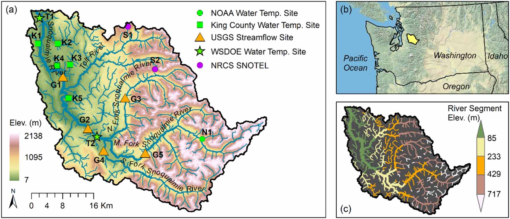
The Snoqualmie River Basin (SRB), located on the west side of the Cascade Mountains, Washington, has three main forks (north, middle, and south) and a drainage size of about 1800 km2 (figure 1). The SRB has a Mediterranean climate with precipitation occurring predominantly from October to March. Elevation ranges from 7 m to 2138 m, and the strong elevational temperature gradient controls the phase of winter precipitation, leading to a mix of rain-dominated, rain-snow transient, and snow-dominated zones (Jefferson 2011). In the alpine area, ground soil surface is directly underlain by bedrock units that do not contain significant fracture systems, indicating that rain and snowmelt do not infiltrate deeply but are transmitted to the stream system rapidly (Turney et al 1995, Bethel 2004). Snoqualmie Falls, downstream on the mainstem after the three forks converge, signals a transition from forest toward anthropogenic impacts including residential, commercial, and agricultural land use. The watershed provides habitat to five anadromous Pacific salmon: Chinook (Oncorhynchus tschawytcha), chum (O. keta), coho (O. kisutch), pink (O. gorbuscha), and winter steelhead (O. mykiss) (Steel et al 2016, Lee et al 2020).

Figure 1. (a), (b) Location of SRB and gage stations of streamflow, snow, and water temperature used for DHSVM-RBM parameterization and evaluation. (c) Elevation of stream segments across the river network.
Download figure:
Standard image High-resolution image2.2. Data sources
2.2.1. In situ data for model calibration and validation
We obtained in situ streamflow, snow, and stream temperature data from multiple agencies across the basin for model calibration and validation (figure 1(a)). Specifically, daily snow water equivalent (SWE) data were acquired from two Natural Resources Conservation Service Snow Telemetry (SNOTEL) stations (S1, S2 ) within the basin. The SWE data (1994–2013) were quality controlled and bias corrected for snowfall undercatch following the approaches outlined in Yan et al (2018) and Sun et al (2019). Daily streamflows (1992–2013) were acquired from five US Geological Survey (USGS) flow gauges (G1–G5); stream temperatures were obtained from Washington State Department of Ecology (WSDOE, T1, T2), King County (K1–K5), and National Oceanic and Atmospheric Administration (NOAA, N1). These datasets are distributed across the basin from tributaries to the mainstem. Two WSDOE sites on the mainstem provided daily stream temperature in summertime during 2002 and 2010. Five King County sites were located in the tributaries in the lower SRB and provided continuous daily stream temperature with different start dates from 2000 to 2009. The NOAA site, located in the alpine area and sensitive to snowmelt effects, provided 30 min stream temperature since 2011.
2.2.2. Meteorological forcing
The 1/16° meteorological forcing data consisting of daily precipitation, maximum and minimum temperature, and wind speed, were acquired from Livneh et al (2013) with temporal coverage 1950–2013. To project future changes, we used the multivariate adaptive constructed analogs (MACA) statistically downscaled coupled model intercomparison project phase 5 (CMIP5) general circulation model (GCM) products (Abatzoglou and Brown 2012). Among the 20 downscaled GCM products bias corrected to the Livneh historical dataset, we selected the top ten GCMs that better reproduced past climate in the PNW for the representative concentration pathways (RCP) 8.5 scenario (Rupp et al 2013, Lee et al 2020). The selected ten GCMs are presented in table 1. All downscaled GCM products had the same meteorological variables as the Livneh dataset with temporal coverage 1950–2005 for the historical period and 2006–2099 for the RCP 8.5 projection.
Table 1. Data sources used for DHSVM-RBM model configuration and projection.
| Data | Source | Application |
|---|---|---|
| National Elevation Data Set (NED) (30 m) | US Geological Survey | DHSVM—digital elevation model (DEM) |
| State Soil Geographic (STATSGO) | US Department of Agriculture | DHSVM—soil characteristics |
| National Land Cover Database (NLCD) for year 2003 (30 m) | US Geological Survey | DHSVM—vegetation information |
| 150-feet L and cover data along each side of the mainstem | Washington State Department of Ecology | RBM—existing riparian information |
| Terra color world imagery (15 m) | Environmental Systems Research Institute | RBM—existing riparian information |
| Streamflow data at G1–G5 (see figure 1) | US Geological Survey | RBM—Leopold coefficients |
| Water temperature data at K1–K5 (see figure 1) | Washington State King County | RBM—Mohseni coefficients |
| GCM: bcc-csm1-1-m | MACAv2-LIVNEH dataset, University of Idaho | Forcing data for DHSVM—RBM: project future changes |
| GCM: CanESM2 | ||
| GCM: CCSM4 | ||
| GCM: CNRM-CM5 | ||
| GCM: CSIRO-Mk3-6-0 | ||
| GCM: HadGEM2-CC365 | ||
| GCM: HadGEM2-ES365 | ||
| GCM: IPSL-CM5A-MR | ||
| GCM: MIROC5 | ||
| GCM: NorESM1-M |
2.3. Coupled hydrology and stream temperature modeling
A modified version of DHSVM-RBM, which integrates the physics-based hydrological model DHSVM and a vector-based semi-Lagrangian stream temperature model RBM, was used for modeling hydrology and stream temperature over the SRB. The original model neglected the thermal effect of cool snowmelt runoff, which can introduce nontrivial errors in temperature simulations for snow-influenced mountain watersheds like SRB. To address this issue, DHSVM-RBM was modified to account for snowmelt thermal influence from upstream boundary conditions along longitudinal flow paths by advection across the river network. Given a considerable body of literature detailing the physics, formulations and parameterization of DHSVM and RBM (Wigmosta et al 1994, Yearsley 2009, 2012, Sun et al 2015, Yearsley et al 2019), we describe the model components briefly below.
The hydrological model DHSVM (Wigmosta et al 1994) solves the water and energy balance at every pixel for simulating key surface and subsurface hydrological processes. It contains a two-layer energy balance snow model for simulating snow accumulation and melt, a two-layer canopy model for modeling interception and evapotranspiration, a multi-layer unsaturated soil model for modeling vertical soil water distribution, and a saturated lateral subsurface flow model. Surface and subsurface flow is routed downslope driven by topography until reaching the channel network, where it is then routed using a cascade of linear reservoirs (Wigmosta et al 2002). For the SRB application, DHSVM was implemented at a three-hourly temporal scale and 150 m spatial scale, forced by meteorological variables including precipitation, air temperature, wind speed, relative humidity, downward shortwave and longwave radiation, which were disaggregated using the mountain microclimate simulation model (Hungerford et al 1989) from the daily meteorological data (both historical and GCM downscaled). The channel network represented by connected river segments generated from a digital elevation model is used by RBM to establish the topology for the semi-Lagrangian particle tracking scheme in advection-dominated river systems.
Originally, DHSVM provided to RBM the segment-specific time series of forcing data consisting of air temperature, shortwave and longwave radiation, wind speed and vapor pressure, and inflow and outflow simulations for each river segment throughout the river network. Here, we modified DHSVM to provide to RBM additional time series input of segment-specific snow melt to identify melt influenced locations and the magnitude of melt.
RBM simulates water temperature dynamics by solving the one-dimensional, time-dependent equations for the thermal energy budget:
where T is water temperature (°C) at time t+ Δt and distance x; Δt is the time increment for a Lagrangian parcel to travel from the upstream starting point to the downstream location x determined by flow velocity u(t, x) (m s−1); D(t, x) is water depth (m); ρ is the density of water (kg m−3); Cp is the specific heat capacity of water (J kg−1 °C−1); F[] represents thermal energy budget components that are a function of T, given by:

where Hcon is thermal energy flux due to conduction, Hback is the flux due to longwave radiation from the water surface, and Hevap is the flux from the latent heat loss due to evaporation; h[] represents the known inputs to the thermal energy balance that are not a function of T, given by:

where Hsw is the net shortwave solar radiation reaching the water surface after attenuation from topography and riparian vegetation, and Hlw is the downward longwave radiation from the atmosphere; and B[] represents advected sources of thermal energy from tributaries and lateral surface/subsurface flows, given by:

where Strib and Slat is the ratio of the volume of tributary and lateral inflows to the segment volume, respectively; Ttrib and Tlat is the water temperature of the tributary and lateral inflows, respectively. With the model modification, when the snowpack melted (i.e. DHSVM simulated local melt for a river segment exceeds a user-specified depth threshold), Tlat were assumed to be snowmelt runoff with a constant temperature of 0.1 °C (Kobayashi 1985, Ficklin et al 2012). Otherwise, the mean annual air temperature was used as a proxy for Tlat.
Estimation of initial conditions (headwater temperatures) was modified to use snowmelt temperature of 0.1 °C during snowmelt, and the nonlinear regression model of Mohseni et al (1998) was used in the absence of melt:
where Thead is daily headwaters temperature (°C), Tsmooth is smoothed air temperature (°C). Mohseni parameters α, β, μ, γ were estimated and tuned based on multi-year observations of air temperature and water temperature records from K1–K5 stations. With no available observations of headwater temperatures in the upper SRB, we used headwater measurements from a nearby watershed (USGS gauge ID: 12116500).
Segment-specific hydraulic characteristics (i.e. U and D) were estimated from DHSVM streamflows using the power law relationships from Leopold and Maddock (1953):

where Q is segment streamflow, and the parameters, da, db, ua and ub were initialized based on stage-discharge relationships derived from five USGS sites (G1−G5 in figure 1). Both Leopold and Mohseni parameters estimated at the individual gauges were extended to their nearby stream segments with no local observations. Sources of key input data to DHSVM-RBM are presented in table 1.
2.4. Fish growth potential modeling
We used simulated water temperatures from DHSVM-RBM to demonstrate how growth potential for native coldwater Chinook salmon, coho salmon, steelhead, pink salmon, and one nonnative warmwater species, largemouth bass, may change in a future climate. For each species, we estimated growth potential for a 1 g fish in each reach accessible to fish twice daily at 6am and 6pm using the Wisconsin bioenergetics model (Hanson et al 1997). Growth is affected by fish mass, water temperature, food availability, and the energy density of predators and prey. In our scenarios, only water temperature varied. We calculated potential food availability in each reach as the product of stream order and distance upstream, which ranged between a maintenance ration and a maximum consumption ration. We used standard bioenergetics modeling options (Hanson et al 1997), and default values for most parameters (table S1 (available online at stacks.iop.org/ERL/16/054006/mmedia)). We used updated temperature-dependent consumption parameters for Chinook salmon provided by Plumb and Moffitt (2015) because these better represent PNW juveniles and we increased the prey energy density parameter from the default value of 2500 J g−1 to 3000 J g−1 to better match salmon prey in the wild (Beauchamp et al 2007). We summarized seasonal growth potential for each species, focusing on longitudinal patterns in the mainstem from the river outlet to Snoqualmie Falls. We did not consider potential fish movement or other ecological factors that influence growth in the wild. Here, our aim was not to predict actual fish growth, but to illustrate relative changes in growth potential across seasons throughout the mainstem that reflect thermal changes associated with different climate scenarios.
3. Results and discussion
3.1. DHSVM-RBM evaluation
DHSVM-RBM was run from 1 October 1990 to 31 December 2013 with the first two years as a spin-up period. Streamflow in the first six water years (1992–1998) at station G1 were used for model calibration, and the model was validated for the remaining 15 water years (1998–2013) at G1 and all streamflow records collected at G2–G5 from 1992 to 2013. Given shorter durations of stream temperature measurements, full records at the two sites (T1, T2) were used for calibration. Details of the calibration procedure are provided in the supplementary information.
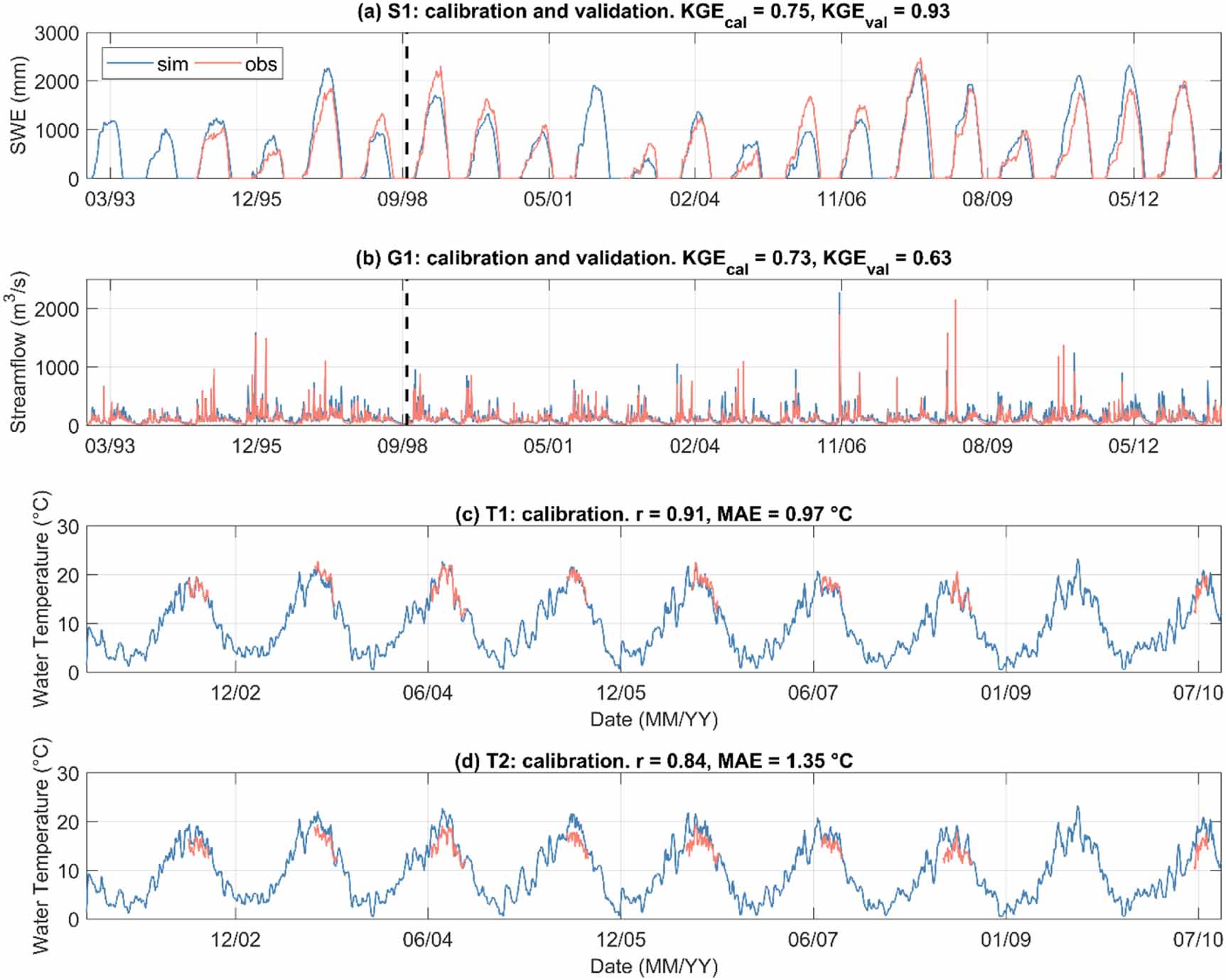
Figure 2 presents DHSVM-RBM calibration and validation results for selected snow, streamflow, and water temperature sites. Full calibration and validation results for all sites are shown in figures S1–S3. For calibration, the daily SWE Kling–Gupta efficiency (KGE, equation S1) was 0.75 and 0.72 for S1 and S2, respectively; the daily streamflow KGE was 0.73 for G1. Model performance in the validation periods was slightly degraded compared to calibration. The daily SWE KGE was 0.93 for S1 and 0.67 for S2; the daily streamflow KGE ranged from 0.60 to 0.65 for G1–G5. Simulated daily water temperatures for the five tributary sites (K1–K5) had Pearson's correlation coefficients (r) of 0.94–0.96 and mean absolute error (MAE) of 0.92 °C–1.43 °C; the r for the two mainstem sites (T1 and T2) was 0.91 and 0.84, and MAE was 0.97 °C and 1.35 °C, respectively. The results suggest that DHSVM-RBM-simulated snow, hydrologic and stream temperature predictions match in situ observations fairly well across the basin.
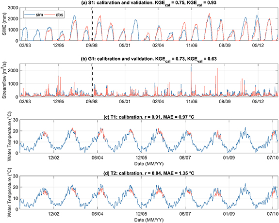
Figure 2. DHSVM-RBM calibration and validation results for selected snow, streamflow, and water temperature sites as examples. Model simulated snow and streamflow were evaluated by the KGE, and stream temperatures simulations were evaluated by the MAE and the Pearson correlation coefficient (r). Black dashed lines in (a) and (b) divide the calibration (left) and validation (right) periods.
Download figure:
Standard image High-resolution image3.2. Snowmelt effects on stream temperature
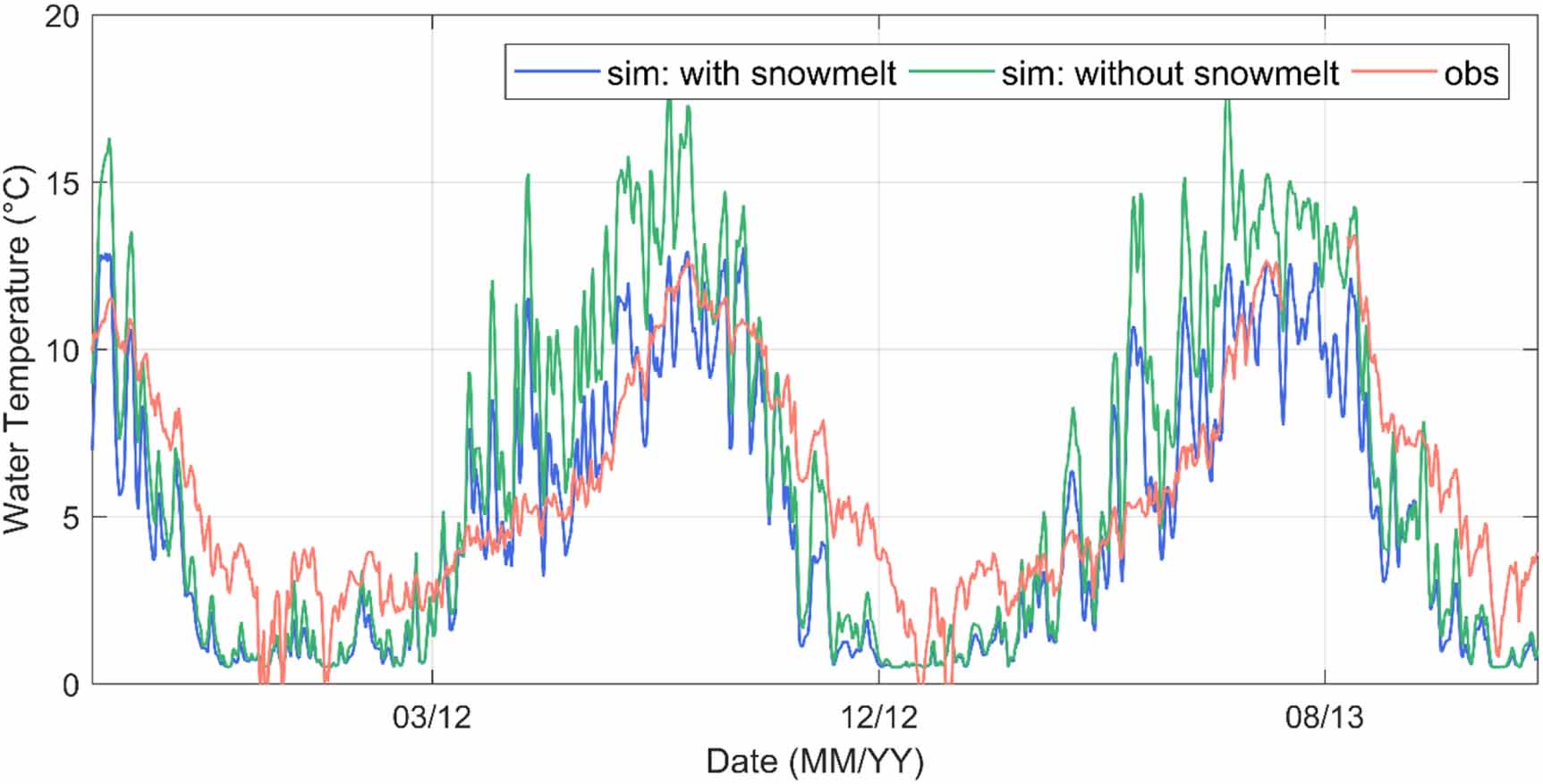
Figure 3 compared stream temperature simulations during 2011–2013 with and without considering snowmelt effects for the N1 site which is in the alpine area with seasonal snow cover. Results suggest that during the snowmelt season from March through August, simulations that did not include snowmelt effects showed substantial overestimation of observed stream temperatures. Accounting for snowmelt effects helped to correct these biases: the MAE of simulated daily stream temperature and the absolute error of 7-DADMax decreased from 2.4 °C and 3.4 °C without snowmelt effects to 2.0 °C and 0.1 °C with snowmelt effects considered, respectively. Although the overall streamflow in SRB has limited contributions from deep groundwater (Leibowitz et al 2016), field surveys confirmed that some locations in the river were potentially influenced by localized hyporheic exchange and/or groundwater inputs (King County 2016, McGill et al 2021). Not representing thermal input from hyporheic exchange or deep groundwater in confined aquifers in DHSVM-RBM may explain the generally overestimated diurnal range of river temperatures, and the underestimated winter stream temperatures.

Figure 3. DHSVM-RBM stream temperature simulation results for N1 site with and without considering snowmelt effects.
Download figure:
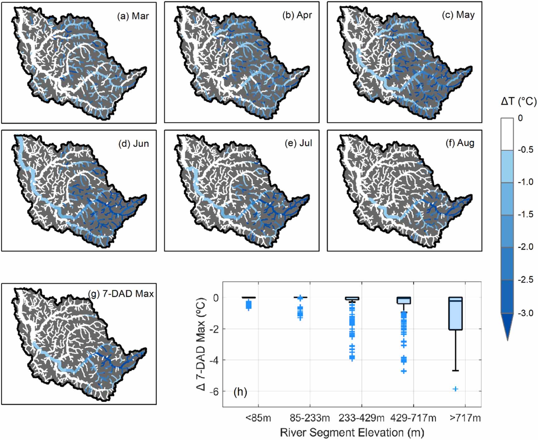
Standard image High-resolution imageFigure 4 presents the basin-wide monthly mean stream temperature changes between two simulations (with snowmelt minus without snowmelt) from March to August over 2001–2013. As observed in figures 4(a)–(f), beginning in March snow in the low-to-moderate elevations starts to melt. In early snowmelt periods, cool snowmelt water has a major influence on temperatures of headwaters and lower-order tributaries. As air temperatures continue to rise, the spatial extent and rates of melt increase, resulting in amplified effects of cool snowmelt water extending from tributaries to the mainstem from advection. By June, the model suggests that snowmelt from upstream rivers reduces the basin outlet stream temperature by about 0.5 °C. Towards the end of the melt season (July to August), snowmelt cooling effects start to recede and occur mainly in the highest elevations (i.e. reducing Middle Fork temperatures by 2.6 °C to 3.4 °C).

Figure 4. (a)–(f) Monthly mean stream temperature changes between two simulations (with snowmelt minus without snowmelt) from March to August over 2001–2013. (g) Changes of basin-wide 7-DADMax between two simulations, and (h) boxplots of basin-wide changes of 7-DADMax grouped by the five elevation bands shown in figure 1(c).
Download figure:
Standard image High-resolution imageComparisons were also made in simulated basin-wide 7-DADMax with and without considering snowmelt effects, which were summarized by five elevation bands of the SRB shown in figure 1(c) (figures 4(g) and (h)). Results suggest that snowmelt generally has greater cooling effects on the 7-DADMax of up to 5.8 °C for streams at higher elevations such as the Middle Fork drainage, and a cooling effect of >0.5 °C extends downstream until near the confluence of the Tolt River. For example, the differences of 7-DADMax are −1.0 °C at the elevation band >717 m, as compared to −0.1 °C at the elevation band of <85 m (most of which are downstream of the lower Snoqualmie-Tolt River confluence). At elevations higher than 717 m, with snowmelt influence considered, about 33% and 26% of stream segments showed a decrease in 7-DADMax greater than 1.0 °C and 2.0 °C, respectively. This spatial variability of snowmelt influence on 7-DADMax, which occurred during July and August in all river segments, is related to the timing and rates of snowmelt from both the local reach and its upstream contributing reaches. High elevation areas such as the Middle Fork subbasin are characterized by higher snow accumulations and later onset of above-freezing air temperatures. This topographical influence resulted in greater snowmelt late into the summer that was able to reduce 7-DADMax locally and downstream as melt runoff traveled along its flow path.
3.3. Projected hydrologic and stream temperature changes
For consistency with the historical stream temperature simulations, we also used a 13 year period to estimate the potential changes of stream temperature under a warming climate. We ran DHSVM-RBM using ten GCM ensembles for a historical period (1993–2005) and a future period at the end of century (2087–2099).
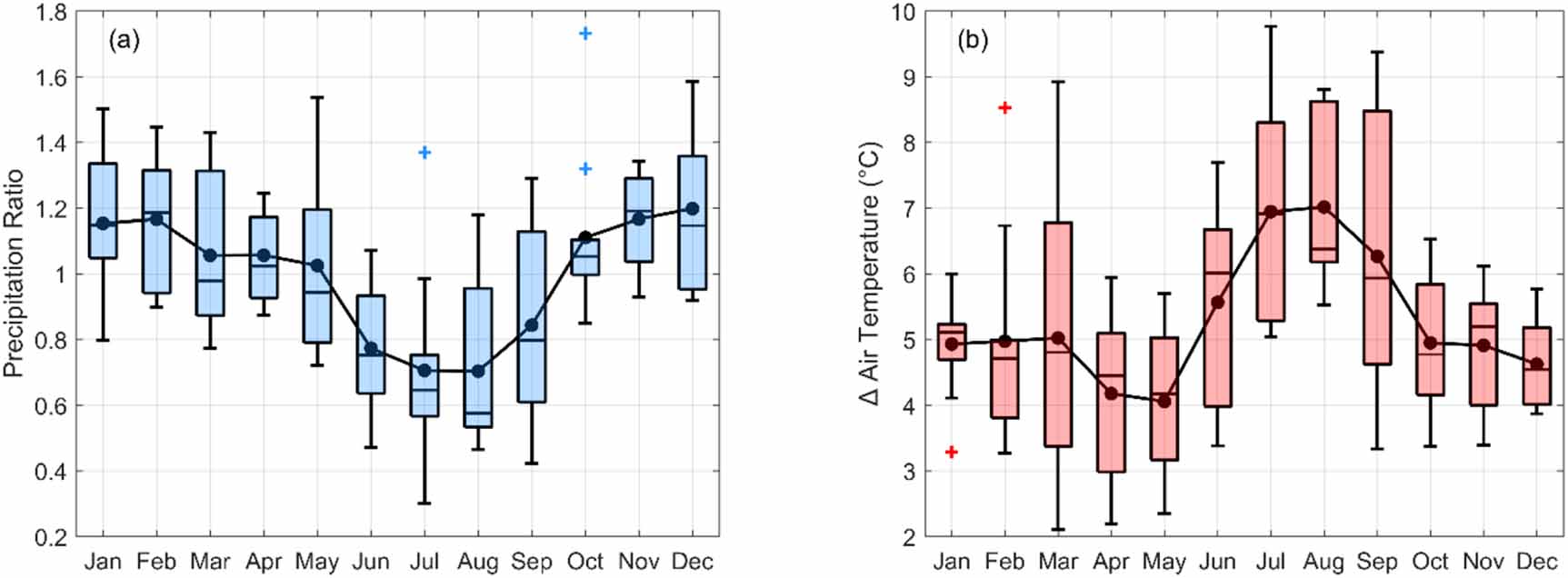
Figure 5 presents the changes of monthly precipitation and air temperature between historical and future projections based on ten GCMs averaged over the basin. It is projected that the mean annual temperature over the basin will increase by 4 °C–7 °C by the end of the century with the largest increases occurring during the summer months. Most GCMs project increased precipitation of up to 58% during the winter and early spring and substantially decreased precipitation of up to 70% during the summer months. Similar to previous studies (Tohver et al 2014, Mote et al 2018, Yan et al 2019b, Lee et al 2020), the model suggests that the SRB shifts from a snow-influenced basin to a rain-dominated basin in future climates. Over the basin, the mean snow accumulation decreases substantially (i.e. 92% reduction in peak SWE) as a result of warming, which prompts earlier onset of snowmelt by about 2 months and earlier disappearance of snow cover (figure 6). Alterations in snowpack along with changing climate result in higher streamflows in winter and early spring, and significantly lower streamflows from late spring through fall (figure S4). For example, summer streamflow in the high-altitude Middle Fork is projected to decrease by 52%–82%. Overall, river segments at higher elevations, where snow regimes exert a greater influence on streamflow, exhibit greater streamflow seasonal variability in response to changing climates (figure S5).

Figure 5. Boxplots of ten GCMs' basin mean monthly precipitation ratio (future/historical) and air temperature change (future − historical). Historical period: 1993–2005. Future period: 2087–2099 under RCP8.5. The dots indicate the ten GCM ensemble mean values.
Download figure:
Standard image High-resolution image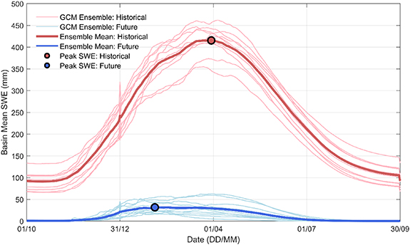
Figure 6. Ten GCMs (thin line) and ensemble mean (thick line) of basin mean SWE over historical (1993–2005) and future (2087–2099) periods under RCP8.5 scenario. Dots indicate ensemble mean annual peak SWE date for both historical (30th March) and future (3rd February) periods.
Download figure:
Standard image High-resolution imageFigure 7 shows the changes in 7-DADMax, comparing future and historical periods for each stream segment across the basin. Consistent with Steel et al (2019), simulations suggest that 7-DADMax will not uniformly increase in the future over the SRB basin; increases are projected to be most prevalent in the snow-dominated high elevation areas (e.g. Middle Fork) and the downstream mainstem until the convergence with the Tolt River. This is due to the compound effect of increasing heatwave events both in duration and intensity, diminishing snowpack and thus reduced snowmelt cooling effects in summer, as well as diminished streamflow from decreasing precipitation and snowpack. It should be noted that our findings are not consistent with previous studies, that analyzed multi-year stream temperature observations for interannual correlations with air temperature and found that cold streams are less sensitive to air temperature variation mainly due to snowmelt input (Isaak et al 2010, Isaak and Rieman 2013, Luce et al 2014). The changing sensitivity of snow-dominated streams to a warming climate reflects a 'tipping point' that the long-term model projection captures but short data records may not, especially during extreme hydrometeorological events. For example, the recent 2015 drought in Washington State provided a useful harbinger of the future (Marlier et al 2017). In 2015, Washington State experienced extreme drought attributed to high winter air temperature that resulted in exceptionally low winter snowpack in the Cascades Range. Steel et al (2019) compared 2015 stream temperature observations to more typical conditions (2012–2014) throughout the Snoqualmie River and found that the largest changes for summer temperature occurred in the snowmelt-dominated Middle Fork.
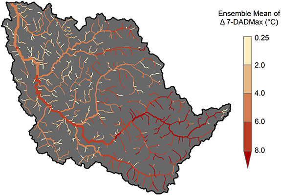
Figure 7. Ten GCM ensemble mean change (future − historical) of 7-DADMax for each stream segment across the basin. Historical period: 1993–2005. Future period: 2087–2099 under RCP8.5.
Download figure:
Standard image High-resolution image3.4. Projected fish habitat changes
Based on the Washington State Legislature spawning rearing and migration criteria (figure S6), we found that river temperature exceeding the state standards dominated in the summer season, and about 65% of the river segments (70% of anadromous-accessible reaches) over the basin fail to meet the water quality standard in the historical summer period and this number will increase to 92% by the end of the 21st century averaged over the ten GCMs; the basin average number of days exceeding the state standards annually will increase substantially from 77 (86) to 135 (143) d (figure S7). Our bioenergetics modeling suggested that warmer future stream temperatures could enhance growing opportunities during winter; however, the increasing air temperature coupled with loss of snow-cooled water during late spring and summer will substantially lower growth potential for coldwater salmonids (figure 8). High future summer temperatures may be more detrimental for some species than others. For instance, pink salmon smolts enter marine waters in spring, whereas coho, steelhead, and some runs of Chinook remain in streams during summer. Warmwater species such as largemouth bass are likely to experience minor increases in habitat suitability year-round, which could compound risks to juvenile salmon if warmer temperatures increase largemouth bass's energetic needs and if newly thermally suitable habitat expands their range and encroaches on salmon habitat (Hawkins et al 2020). We noted a longitudinal decrease in summer growth potential progressing downstream for Chinook and steelhead, suggesting the substantial loss of coldwater habitats in summer.

Figure 8. Longitudinal change (future − historical) in seasonal growth potential for four native coldwater salmonids and one nonnative warmwater centrarchid in the Snoqualmie River watershed. Plots show medians (dark lines) and 95% percentiles (shaded areas) across ten global climate models, versus distance upstream from the river outlet to Snoqualmie Falls (an anadromous fish barrier). Pink salmon are not present in streams during summer.
Download figure:
Standard image High-resolution image
4. Conclusions
This paper presents a model-based study that addresses the thermal effect of cool snowmelt runoff on river temperatures. As applied to a snow-fed river basin in the PNW, DHSVM-RBM was used to provide a process-guided understanding of climate change impacts on the hydrological system, stream thermal regime, and fish habitats. We showed that snowmelt-cooling effects are critical in stream thermal modeling in snow-dominated watersheds where snowmelt can noticeably reduce the basin-wide 7-DADMax by up to 5.8 °C in high-elevation tributaries, and the cooling effect can sustain until summer in the mainstem as far as the basin outlet. In future climates informed by ensemble GCM projections, we found that snowmelt river segments located in high-elevation areas are most vulnerable to climate change and are projected to experience the largest increase in 7-DADMax across the basin. Projected thermal habitat changes also indicated that growth potential for coldwater anadromous salmonids will be substantially lower in future summers.
Last, interpretation of simulations should take into consideration model limitations as applied in different settings. For example, DHSVM-RBM does not entail process representation of confined aquifers or hyporheic exchange on hydrology and temperature modeling. The approach we developed here to represent melt water thermal influence is simplistic for representing complex processes in nature, however, it has been proven effective for producing reasonable simulations of stream temperatures with snow influence across different scales (Haag and Luce 2008, Ficklin et al 2012, Wu et al 2012). In the context of watershed or regional applications, a simplified process representation with reduced parameterization also helps to maintain reasonable computational time and avoid model over-parameterization, given that spatially continuous observations required for proper initialization, parameterization and validation of complex processes are largely lacking.
Acknowledgments
This work is supported by the US Bureau of Indian Affairs through Grant No A18AP00192, issued to the Snoqualmie Indian Tribe. Battelle Memorial Institute operates the Pacific Northwest National Laboratory (PNNL) for the US Department of Energy under contract DE-AC06-76RLO-1830.
Data availability statement
The DHSVM-RBM source code and bias-corrected quality-controlled (BCQC) SNOTEL data used in this paper are (available at https://dhsvm.pnnl.gov/). The USGS streamflow data are (available at https://waterdata.usgs.gov/nwis/sw/). The WSDOE water temperature data are (available at https://ecology.wa.gov/Research-Data). The Washington State King County and NOAA water temperature data are (available at https://green2.kingcounty.gov/hydrology/). The Livneh 1/16° meteorological forcing data are (available at https://ciresgroups.colorado.edu/livneh/data). The MACA downscaled GCM products are (available at www.climatologylab.org/maca.html.